
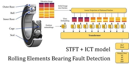
A Combined Short Time Fourier Transform and Image Classification Transformer Model for Rolling Element Bearings Fault Diagnosis in Electric Motors


Abstract
1. Introduction
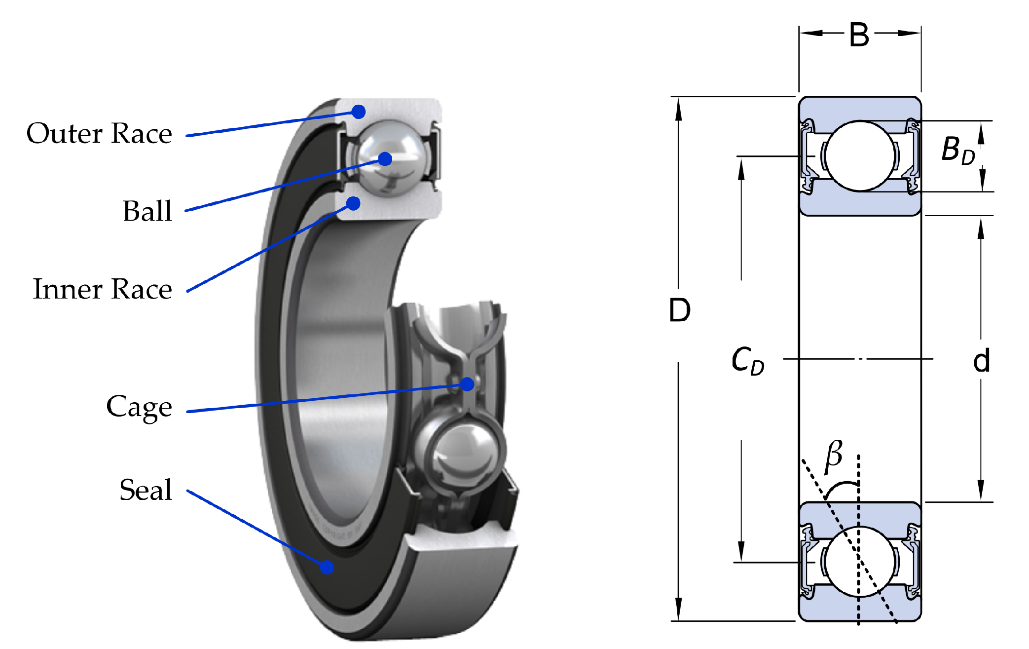
2. Bearing Faults
- Characteristic frequency of the ball fault:
- Characteristic frequency of the inner race fault:
- Characteristic frequency of the outer race fault:
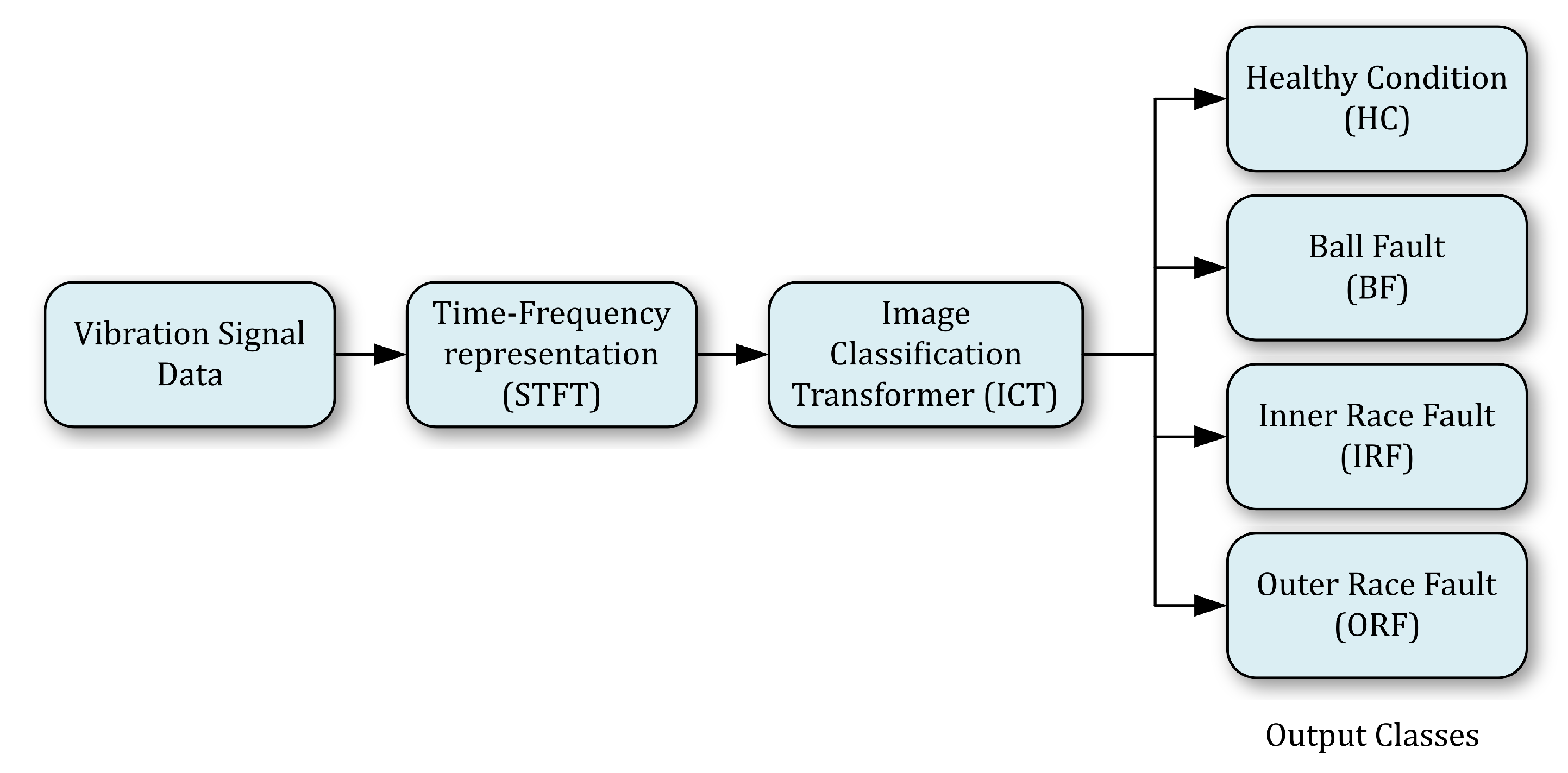
3. Methodology and Materials
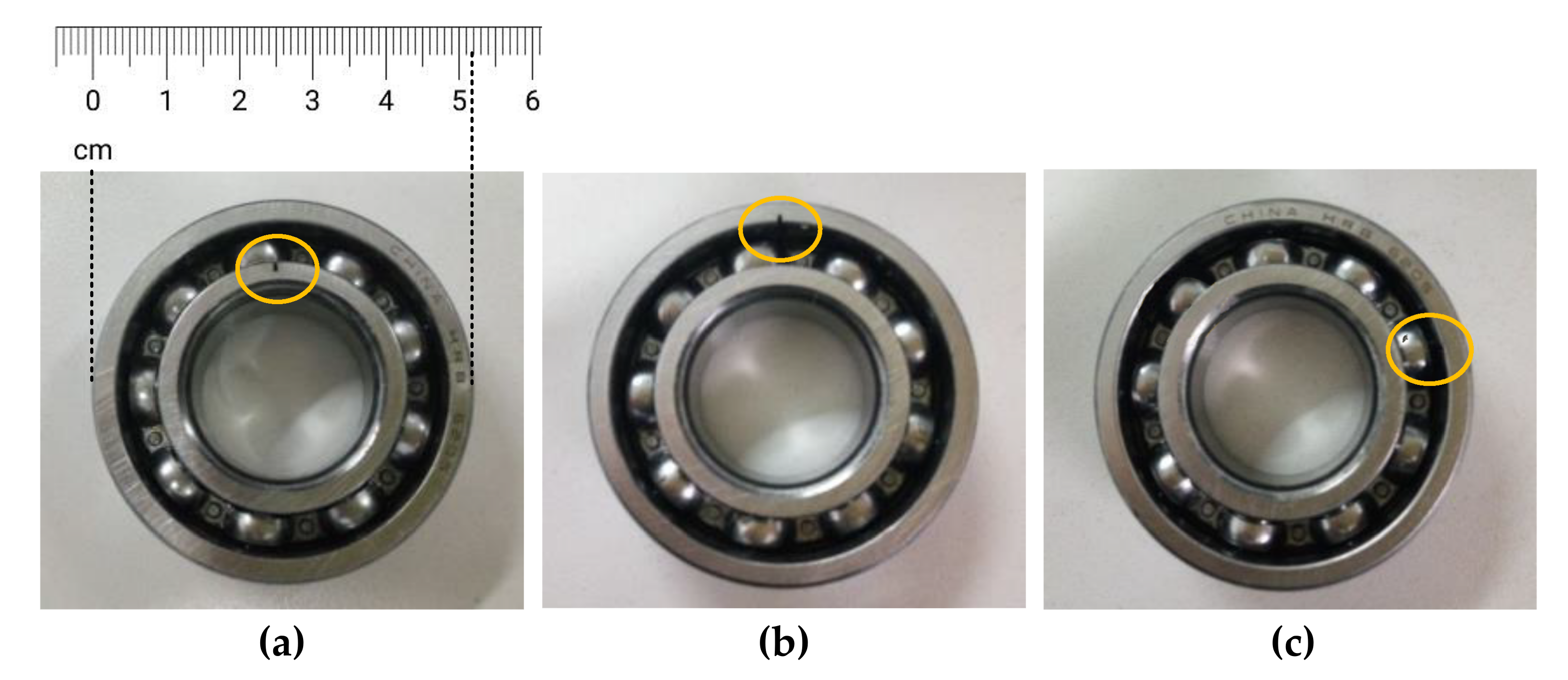
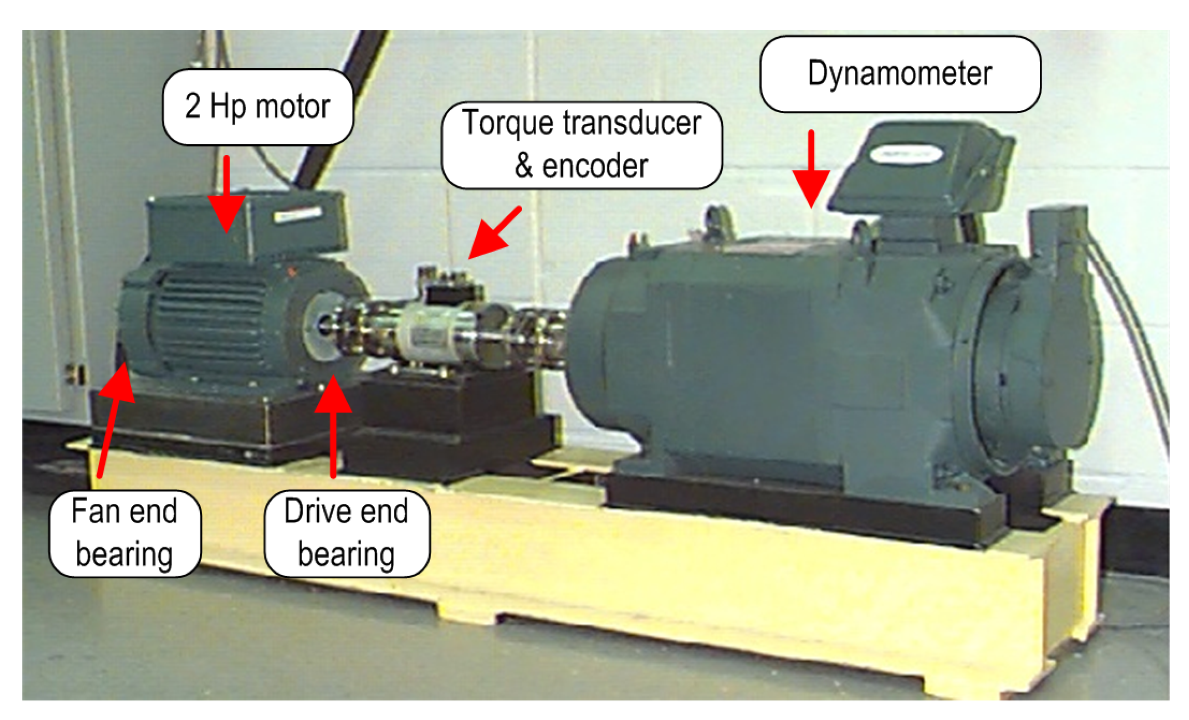
3.1. Vibration/Acceleration Data and Characteristics
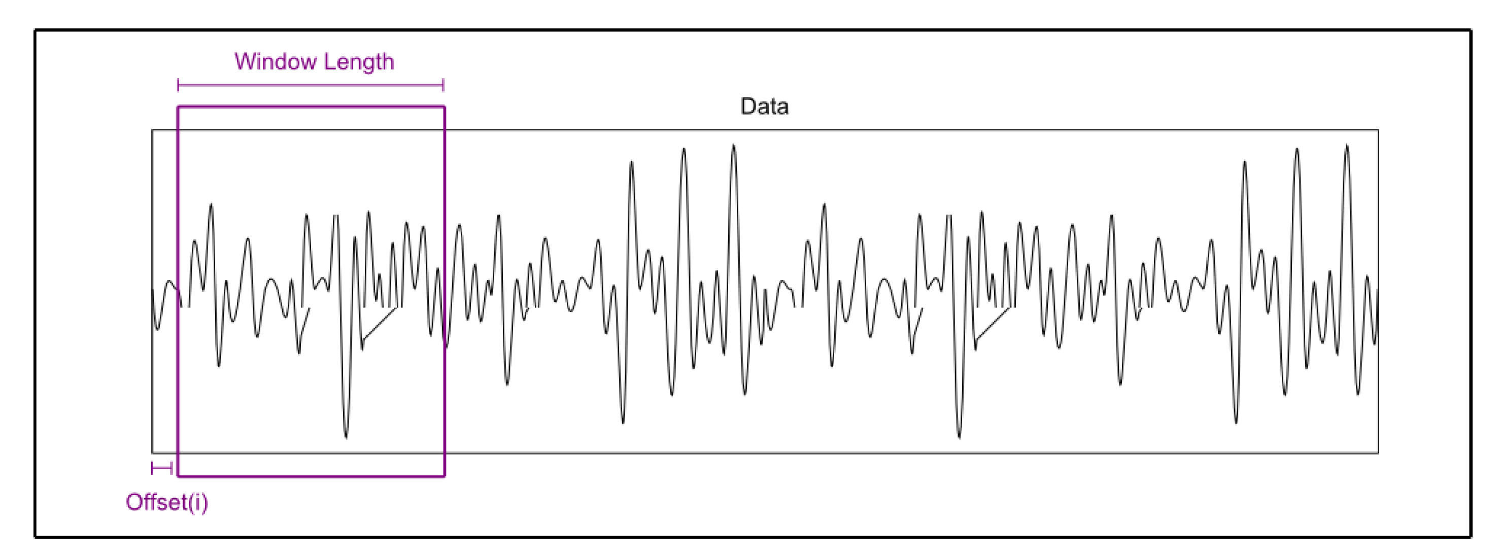
3.2. Pre-Processing Using STFT
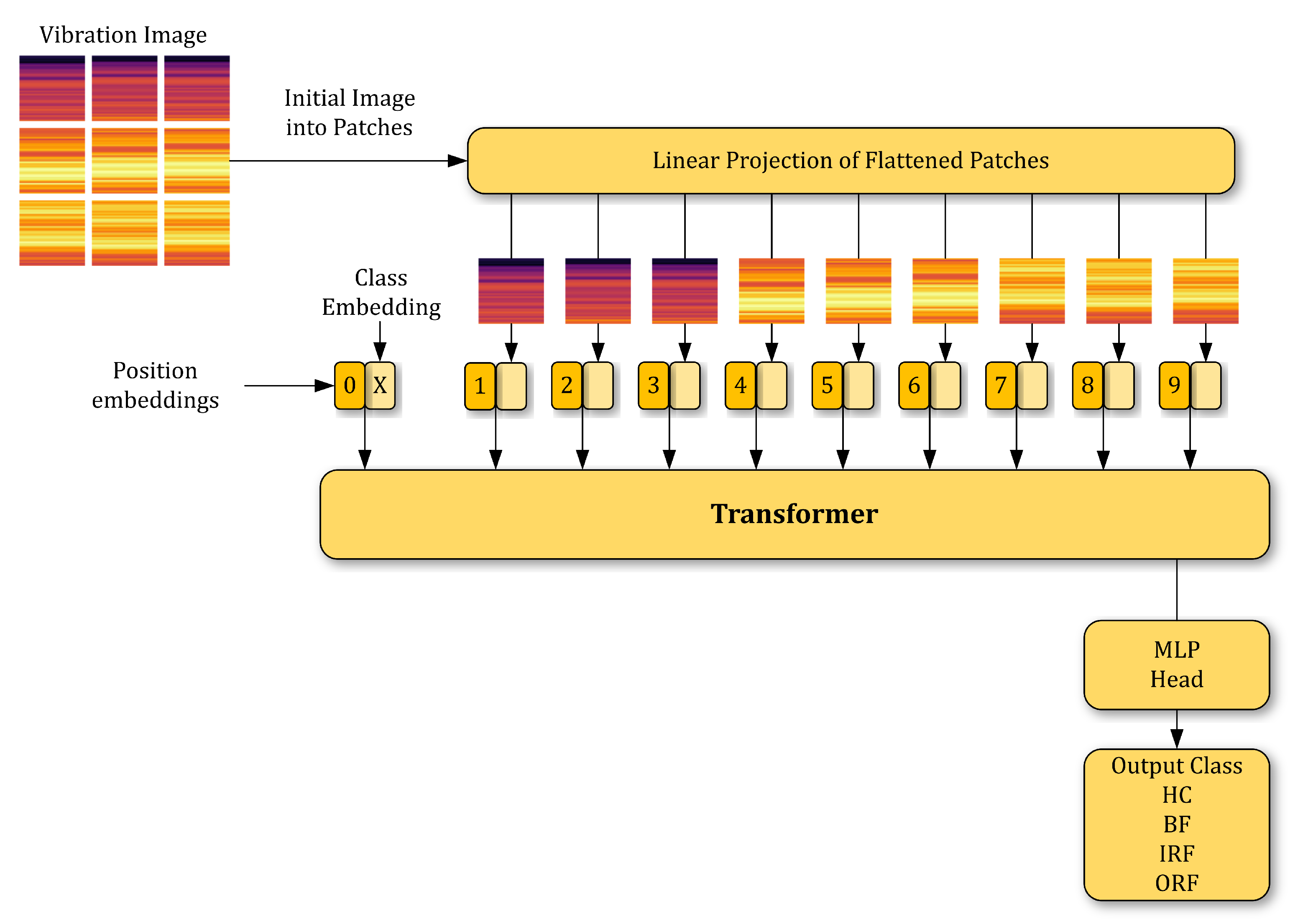
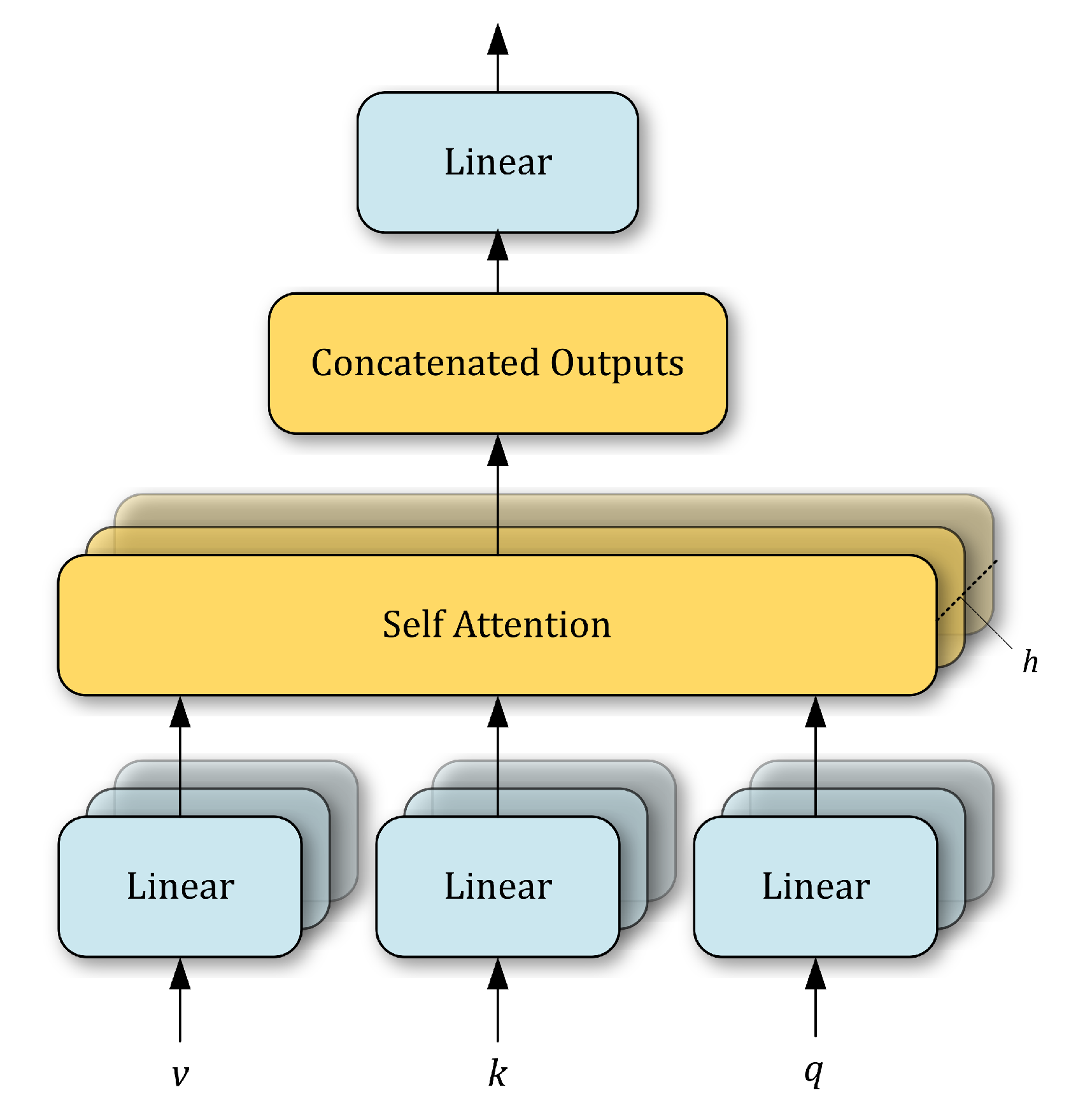
3.3. Image Classification Transformer
4. Experimental Results and Discussion
Comparison with Other Models and Methods
5. Conclusions and Future Work
Author Contributions
Funding
Data Availability Statement
Acknowledgments
Conflicts of Interest
Abbreviations
| ANFIS | Adaptive Neuro-Fuzzy Inference System |
| IRF | Inner Race Fault |
| BF | Ball Fault |
| KNN | k-Nearest Neighbor |
| CBM | Condition-Based Maintenance |
| MAS | Multi Agent System |
| CNN | Convolutional Neural Network |
| ML | Machine Learning |
| CWRU | Case Western Reserve University |
| MLP | Multi-Layer Perceptron |
| DBN | Deep Belief Networks |
| MSA | Multi-head Self-Attention |
| DNN | Dense Neural Networks |
| NLP | Natural Language Processing |
| FCN | Fuzzy Cognitive Networks |
| ORF | Outer Race Fault |
| GMAC | billions of Mac (multiply+sum operations) |
| PVA | Park’s Vector Analysis |
| GPU | Graphich Processing Unit |
| SA | Self-Attention |
| HC | Healthy Condition |
| SoC | System-on-Chip |
| ICT | Image Classification Transformer |
| STFT | Short Time Fourier Transform |
| IPF | Instantaneous Power Factor |
| SVM | Support Vector Machine |
References
- Dineva, A.; Mosavi, A.; Ardabili, S.F.; Vajda, I.; Shamshirband, S.; Rabczuk, T.; Chau, K.W. Review of Soft Computing Models in Design and Control of Rotating Electrical Machines. Energies 2019, 12, 1049. [Google Scholar] [CrossRef]
- Bazine, S.; Trigeassou, J.C. Faults in Electrical Machines and their Diagnosis. In Electrical Machines Diagnosis; John Wiley & Sons, Inc.: Hoboken, NJ, USA, 2013; pp. 1–22. [Google Scholar] [CrossRef]
- Frosini, L.; Harlisca, C.; Szabo, L. Induction Machine Bearing Fault Detection by Means of Statistical Processing of the Stray Flux Measurement. IEEE Trans. Ind. Electron. 2015, 62, 1846–1854. [Google Scholar] [CrossRef]
- Thorsen, O.; Dalva, M. Failure Identification and Analysis for High-Voltage Induction Motors in the Petrochemical Industry. IEEE Trans. Ind. Appl. 1999, 35, 810–818. [Google Scholar] [CrossRef]
- Henao, H.; Capolino, G.A.; Fernandez-Cabanas, M.; Filippetti, F.; Bruzzese, C.; Strangas, E.; Pusca, R.; Estima, J.; Riera-Guasp, M.; Hedayati-Kia, S. Trends in Fault Diagnosis for Electrical Machines: A Review of Diagnostic Techniques. IEEE Ind. Electron. Mag. 2014, 8, 31–42. [Google Scholar] [CrossRef]
- Neelam, M.; Ratna, D. Detection of Bearing Faults of Induction Motor Using Park’s Vector Approach. Int. J. Eng. Technol. 2010, 2, 263–266. [Google Scholar]
- Ibrahim, A.; Badaoui, M.E.; Guillet, F.; Bonnardot, F. A New Bearing Fault Detection Method in Induction Machines Based on Instantaneous Power Factor. IEEE Trans. Ind. Electron. 2008, 55, 4252–4259. [Google Scholar] [CrossRef]
- Smith, W.A.; Randall, R.B. Rolling Element Bearing Diagnostics using the Case Western Reserve University data: A benchmark study. Mech. Syst. Signal Process. 2015, 64, 100–131. [Google Scholar] [CrossRef]
- Toma, R.N.; Prosvirin, A.E.; Kim, J.M. Bearing Fault Diagnosis of Induction Motors Using a Genetic Algorithm and Machine Learning Classifiers. Sensors 2020, 20, 1884. [Google Scholar] [CrossRef] [PubMed]
- Karnavas, Y.L.; Chasiotis, I.D.; Vrangas, A. Fault Diagnosis of Squirrel-Cage Induction Motor Broken Bars based on a Model Identification Method with Subtractive Clustering. In Proceedings of the 2017 IEEE 11th International Symposium on Diagnostics for Electrical Machines, Power Electronics and Drives (SDEMPED), Tinos, Greece, 29 August–1 September 2017. [Google Scholar] [CrossRef]
- Karatzinis, G.; Boutalis, Y.S.; Karnavas, Y.L. Motor Fault Detection and Diagnosis Using Fuzzy Cognitive Networks with Functional Weights. In Proceedings of the 2018 26th Mediterranean Conference on Control and Automation (MED), Zadar, Croatia, 19–22 June 2018. [Google Scholar] [CrossRef]
- Drakaki, M.; Karnavas, Y.L.; Karlis, A.D.; Chasiotis, I.D.; Tzionas, P. Study on Fault Diagnosis of Broken Rotor Bars in Squirrel Cage Induction Motors: A Multi-Agent System Approach using Intelligent Classifiers. IET Electr. Power Appl. 2020, 14, 245–255. [Google Scholar] [CrossRef]
- Konar, P.; Chattopadhyay, P. Bearing Fault Detection of Induction Motor using Wavelet and Support Vector Machines (SVMs). Appl. Soft Comput. 2011, 11, 4203–4211. [Google Scholar] [CrossRef]
- Deng, L. Deep Learning: Methods and Applications. Found. Trends Signal Process. 2014, 7, 197–387. [Google Scholar] [CrossRef]
- Karnavas, Y.L.; Plakias, S.; Chasiotis, I.D. Extracting Spatially Global and Local Attentive Features for Rolling Bearing Fault Diagnosis in Electrical Machines using Attention Stream Networks. IET Electr. Power Appl. 2021. [Google Scholar] [CrossRef]
- Lei, Y. A Deep Learning-based Method for Machinery Health Monitoring with Big Data. J. Mech. Eng. 2015, 51, 49. [Google Scholar] [CrossRef]
- Carmona, J.M.; Climent, J. Human Action Recognition by Means of Subtensor Projections and Dense Trajectories. Pattern Recogn. 2018, 81, 443–455. [Google Scholar] [CrossRef]
- Kiranyaz, S.; Ince, T.; Gabbouj, M. Real-Time Patient-Specific ECG Classification by 1-D Convolutional Neural Networks. IEEE Trans. Biomed. Eng. 2016, 63, 664–675. [Google Scholar] [CrossRef]
- Hu, X.; Lu, X.; Hori, C. Mandarin Speech Recognition using Convolution Neural Network with Augmented Tone Features. In Proceedings of the The 9th International Symposium on Chinese Spoken Language Processing, Singapore, 12–14 September 2014; pp. 15–18. [Google Scholar]
- Turaga, S.C.; Murray, J.F.; Jain, V.; Roth, F.; Helmstaedter, M.; Briggman, K.; Denk, W.; Seung, H.S. Convolutional Networks Can Learn to Generate Affinity Graphs for Image Segmentation. Neural Comput. 2010, 22, 511–538. [Google Scholar] [CrossRef]
- Gu, J.; Wang, Z.; Kuen, J.; Ma, L.; Shahroudy, A.; Shuai, B.; Liu, T.; Wang, X.; Wang, G.; Cai, J.; et al. Recent Advances in Convolutional Neural Networks. Pattern Recogn. 2018, 77, 354–377. [Google Scholar] [CrossRef]
- Zhao, R.; Yan, R.; Chen, Z.; Mao, K.; Wang, P.; Gao, R.X. Deep Learning and its Applications to Machine Health Monitoring. Mech. Syst.d Signal Process. 2019, 115, 213–237. [Google Scholar] [CrossRef]
- Harlişca, C.; Szabo, L. Bearing Faults Condition Monitoring—A Literature Survey. J. Comput. Sci. Control Syst. 2012, 5, 19–22. [Google Scholar]
- Nguyen, T.P.K.; Khlaief, A.; Medjaher, K.; Picot, A.; Maussion, P.; Tobon, D.; Chauchat, B.; Cheron, R. Analysis and Comparison of Multiple Features for Fault Detection and Prognostic in Ball Bearings. In Proceedings of the 4th European Conference of the Prognostics and Health Management Society, Utrecht, The Netherlands, 3 August–6 July 2018; CCSD: Utrecht, The Netherlands, 2018; pp. 1–9. [Google Scholar]
- Gabor, D. Theory of Communication. Part 1: The Analysis of Information. J. Inst. Electr. Eng.-Part III Radio Commun. Eng. 1946, 93, 429–441. [Google Scholar] [CrossRef]
- Vaswani, A.; Shazeer, N.; Parmar, N.; Uszkoreit, J.; Jones, L.; Gomez, A.N.; Kaiser, L.; Polosukhin, I. Attention is All You Need. arXiv 2017, arXiv:cs.CL/1706.03762. [Google Scholar]
- Ba, J.L.; Kiros, J.R.; Hinton, G.E. Layer Normalization. arXiv 2016, arXiv:stat.ML/1607.06450. [Google Scholar]
- He, K.; Zhang, X.; Ren, S.; Sun, J. Deep Residual Learning for Image Recognition. In Proceedings of the 2016 IEEE Conference on Computer Vision and Pattern Recognition (CVPR), Las Vegas, NV, USA, 27–30 June 2016. [Google Scholar] [CrossRef]
- Hendrycks, D.; Gimpel, K. Gaussian Error Linear Units (GELUs). arXiv 2020, arXiv:cs.LG/1606.08415. [Google Scholar]
- Devlin, J.; Chang, M.W.; Lee, K.; Toutanova, K. BERT: Pre-training of Deep Bidirectional Transformers for Language Understanding. arXiv 2019, arXiv:cs.CL/1810.04805. [Google Scholar]
- Kingma, D.; Ba, J. Adam: A Method for Stochastic Optimization. arXiv 2014, arXiv:cs.CL/1412.6980. [Google Scholar]
- Santos, P.; Maudes, J.; Bustillo, A. Identifying Maximum Imbalance in Datasets for Fault Diagnosis of Gearboxes. J. Intell. Manuf. 2015, 29, 333–351. [Google Scholar] [CrossRef]
- Zhang, W.; Li, X.; Jia, X.D.; Ma, H.; Luo, Z.; Li, X. Machinery Fault Diagnosis with Imbalanced Data using Deep Generative Adversarial Networks. Measurement 2020, 152, 107377. [Google Scholar] [CrossRef]
- Lee, J.H.; Pack, J.H.; Lee, I.S. Fault Diagnosis of Induction Motor Using Convolutional Neural Network. Appl. Sci. 2019, 9, 2950. [Google Scholar] [CrossRef]
- Tra, V.; Kim, J.; Khan, S.A.; Kim, J.M. Bearing Fault Diagnosis under Variable Speed Using Convolutional Neural Networks and the Stochastic Diagonal Levenberg-Marquardt Algorithm. Sensors 2017, 17, 2834. [Google Scholar] [CrossRef]
- Hsueh, Y.M.; Ittangihal, V.R.; Wu, W.B.; Chang, H.C.; Kuo, C.C. Fault Diagnosis System for Induction Motors by CNN Using Empirical Wavelet Transform. Symmetry 2019, 11, 1212. [Google Scholar] [CrossRef]
- Jia, F.; Lei, Y.; Lin, J.; Zhou, X.; Lu, N. Deep Neural Networks: A Promising Tool for Fault Characteristic Mining and Intelligent Diagnosis of Rotating Machinery with Massive Data. Mech. Syst. Signal Process. 2016, 72–73, 303–315. [Google Scholar] [CrossRef]
- Deng, W.; Yao, R.; Zhao, H.; Yang, X.; Li, G. A Novel Intelligent Diagnosis Method using Optimal LS-SVM with Improved PSO Algorithm. Soft Comput. 2017, 23, 2445–2462. [Google Scholar] [CrossRef]
- Shao, H.; Jiang, H.; Zhang, X.; Niu, M. Rolling Bearing Fault Diagnosis using an Optimization Deep Belief Network. Meas. Sci. Technol. 2015, 26, 115002. [Google Scholar] [CrossRef]
- Eren, L.; Ince, T.; Kiranyaz, S. A Generic Intelligent Bearing Fault Diagnosis System Using Compact Adaptive 1D CNN Classifier. J. Signal Process. Syst. 2018, 91, 179–189. [Google Scholar] [CrossRef]
- Li, M.; Wei, Q.; Wang, H.; Zhang, X. Research on Fault Diagnosis of Time-Domain Vibration Signal based on Convolutional Neural Networks. Syst. Sci. Control Eng. 2019, 7, 73–81. [Google Scholar] [CrossRef]


| Bearing Condition Status | Bearing Defect Diameter (Inches) | Load (Hp) | ||||
|---|---|---|---|---|---|---|
| 0 | 1 | 2 | 3 | |||
| Speed (rpm) | ||||||
| 1797 | 1772 | 1750 | 1730 | |||
| HC | - | √ | √ | √ | √ | |
| BF | 0.007 | √ | √ | √ | √ | |
| 0.014 | √ | √ | √ | √ | ||
| 0.021 | √ | √ | √ | √ | ||
| 0.028 | √ | √ | √ | √ | ||
| IRF | 0.007 | √ | √ | √ | √ | |
| 0.014 | √ | √ | √ | √ | ||
| 0.021 | √ | √ | √ | √ | ||
| 0.028 | √ | √ | √ | √ | ||
| ORF | Centered @6 | 0.007 | √ | √ | √ | √ |
| 0.014 | √ | √ | √ | √ | ||
| 0.021 | √ | √ | √ | √ | ||
| 0.028 | - | - | - | - | ||
| Orthogonal @3 | 0.007 | √ | √ | √ | √ | |
| 0.014 | - | - | - | - | ||
| 0.021 | √ | √ | √ | √ | ||
| 0.028 | - | - | - | - | ||
| Opposite @12 | 0.007 | √ | √ | √ | √ | |
| 0.014 | - | - | - | - | ||
| 0.021 | √ | √ | √ | √ | ||
| 0.028 | - | - | - | - | ||
| Bearing Condition | Training Data | Testing Data | Overall Data |
|---|---|---|---|
| Healthy Condition | 140 | 60 | 200 |
| Ball Fault | 544 | 256 | 800 |
| Inner Race Fault | 562 | 238 | 800 |
| Outer Race fault | 966 | 434 | 1400 |
| Overall Data | 2212 | 988 | 3200 |
| Classification Report | |||||
|---|---|---|---|---|---|
| Class | Accuracy () | Precision | Recall | F1 Score | Support |
| HC | 1.00 | 1.00 | 1.00 | 1.00 | 60 |
| BF | 0.98 | 0.99 | 0.98 | 0.98 | 238 |
| IRF | 0.98 | 0.97 | 0.98 | 0.97 | 256 |
| ORF | 0.97 | 0.98 | 0.98 | 0.98 | 434 |
| Total | 0.98 | 0.98 | 0.98 | 0.98 | 988 |
| Predicted Class | ||||||
|---|---|---|---|---|---|---|
| HC | BF | IRF | ORF | Total | ||
| Actual Class | HC | 60 | 0 | 0 | 0 | 60 |
| BF | 0 | 234 | 1 | 3 | 238 | |
| IRF | 0 | 1 | 250 | 5 | 256 | |
| ORF | 0 | 1 | 5 | 428 | 434 | |
| Total | 60 | 236 | 256 | 436 | 988 | |
| Model | Accuracy (Avg.) | Parameters | Computational Complexity | Storage |
|---|---|---|---|---|
| CNN | 97.8% | 355.27 M | 0.41 GMac | 1 GB |
| CNN with max-pooling | 97.2% | 1.79 M | 0.16 GMac | 7 MB |
| ICT (proposed) | 98.3% | 745.22 K | 0.05 GMac | 3 MB |
| Methods | Accuracy |
|---|---|
| Dense Neural Network (DNN) [37] | 80.0% |
| Support Vector Machine (SVM) [38] | 89.5% |
| Deep Belief Network (DBN) [39] | 92.2% |
| 1-D (time domain) CNN (1DtdCNN) [40] | 93.3% |
| 2-D (time domain) CNN (2DtdCNN) [41] | 96.0% |
| Image Classification Transformer (ICT) (proposed) | 98.3% |
Publisher’s Note: MDPI stays neutral with regard to jurisdictional claims in published maps and institutional affiliations. |
© 2021 by the authors. Licensee MDPI, Basel, Switzerland. This article is an open access article distributed under the terms and conditions of the Creative Commons Attribution (CC BY) license (http://creativecommons.org/licenses/by/4.0/).
Share and Cite
Alexakos, C.T.; Karnavas, Y.L.; Drakaki, M.; Tziafettas, I.A. A Combined Short Time Fourier Transform and Image Classification Transformer Model for Rolling Element Bearings Fault Diagnosis in Electric Motors. Mach. Learn. Knowl. Extr. 2021, 3, 228-242. https://doi.org/10.3390/make3010011
Alexakos CT, Karnavas YL, Drakaki M, Tziafettas IA. A Combined Short Time Fourier Transform and Image Classification Transformer Model for Rolling Element Bearings Fault Diagnosis in Electric Motors. Machine Learning and Knowledge Extraction. 2021; 3(1):228-242. https://doi.org/10.3390/make3010011
Chicago/Turabian StyleAlexakos, Christos T., Yannis L. Karnavas, Maria Drakaki, and Ioannis A. Tziafettas. 2021. "A Combined Short Time Fourier Transform and Image Classification Transformer Model for Rolling Element Bearings Fault Diagnosis in Electric Motors" Machine Learning and Knowledge Extraction 3, no. 1: 228-242. https://doi.org/10.3390/make3010011
APA StyleAlexakos, C. T., Karnavas, Y. L., Drakaki, M., & Tziafettas, I. A. (2021). A Combined Short Time Fourier Transform and Image Classification Transformer Model for Rolling Element Bearings Fault Diagnosis in Electric Motors. Machine Learning and Knowledge Extraction, 3(1), 228-242. https://doi.org/10.3390/make3010011