Article

Large Scale Fault Data Analysis and OSS Reliability Assessment Based on Quantification Method of the First Type

by
Yoshinobu Tamura
1,*,† and
Shigeru Yamada
2,†
1
Department of Intelligent Systems, Faculty of Information Technology, Tokyo City University, Tokyo 158-8557, Japan
2
Graduate School of Engineering, Tottori University, Tottori 680-8552, Japan
*
Author to whom correspondence should be addressed.
These authors contributed equally to this work.
Mach. Learn. Knowl. Extr. 2020, 2(4), 436-452; https://doi.org/10.3390/make2040024
Submission received: 19 July 2020 / Revised: 11 October 2020 / Accepted: 12 October 2020 / Published: 20 October 2020
(This article belongs to the Section Data)

Abstract

:
Various big data sets are recorded on the server side of computer system. The big data are well defined as a volume, variety, and velocity (3V) model. The 3V model has been proposed by Gartner, Inc. as a first press release. 3V model means the volume, variety, and velocity in terms of data. The big data have 3V in well balance. Then, there are various categories in terms of the big data, e.g., sensor data, log data, customer data, financial data, weather data, picture data, movie data, and so on. In particular, the fault big data are well-known as the characteristic log data in software engineering. In this paper, we analyze the fault big data considering the unique features that arise from big data under the operation of open source software. In addition, we analyze actual data to show numerical examples of reliability assessment based on the results of multiple regression analysis well-known as the quantification method of the first type.

1. Introduction

A waterfall development model is well-known as the traditional software development style. At present, the software development style has been changed to various development paradigms. In particular, the development style of open source software (OSS) has the unique style such as the OSS project. The OSS project has the development cycle in the flow such as development, version release, usage of users, reporting of bug, checking and modifying of OSS, and release of new version. Recently, the OSS with network connection service is increasing more and more. Thus, the numbers of network-oriented OSS such as cloud service, server, IoT (Internet of Things) device software have been increasing as well as the standalone software.
In the past, various methods based on software reliability growth models have been proposed by several research groups [1,2]. On the other hand, several research papers for OSS reliability assessment have been published [3].
There are many OSS reliability assessment methods based on the stochastic models. In addition, there are several methods based on empirical data analysis [4,5]. In particular, it is very useful for the OSS developers to understand the trend of fault big data recorded on the OSS bug tracking system from the standpoint of bird’s-eye view. The organization of this paper is as follows: Section 2 discusses the relationship between the raw data and categorical one. Section 3 proposes the multiple regression analysis in order to solve the problem in terms of the degree of freedom for the large scale fault data. Section 4 describes and analyzes the forward-backward stepwise selection method by analyzing the fault big data. Section 5 discusses the upper and lower confidence limits based on the typical hazard rate model. Section 6 discusses the characteristics of the proposed method.
Many software reliability assessment methods based on the stochastic model have been proposed by several researchers [6,7,8]. Recently, it is difficult to assess the software reliability because there are various software development styles. Historically, the fault data sets are used for the software reliability assessment. In addition, the software reliability assessment methods based on the measurements of software metrics have been proposed in the past [9,10]. At present, many kinds of fault data have been recorded on the bug tracking system in the case of OSS. In particular, it will be useful for the reliability assessment by using various categorized fault data sets in the case of OSS. We will be able to propose the high accuracy method by integrating the stochastic models and the statistical analysis if we can assess the fault big data from the standpoint of statistical analysis.
As the related works, several research papers have proposed the methods in terms of the upper and lower limits based on software reliability growth models [1,2], and the empirical approach for OSS [3]. However, it is difficult to understand the upper and lower bounds of the stochastic model for the big data because of the problem for the degree of freedom. Generally, the degree of freedom is given by the number of data. However, it is difficult to obtain the degree of freedom from the big data, because the data set is in the large scale. Then, we will be able to use the number of explanatory variables in place of the number of data. In this paper, we propose the data analysis method based on a quantification method of the first type. Then, we focus on the fault big data analysis with a more simple method, because the analyses of fault big data are required to take a lot of time for calculation and analysis. The multiple regression-based model to analyze financial data has been proposed in the financial research area [11,12]. Moreover, the multiple regression analysis is used in the research area of network [13]. In this way, the statistical methods such as the multiple regression analysis have been applied to various research areas. This paper proposes the method based on the statistical analysis and typical hazard rate model for the large scale fault data analysis and OSS reliability assessment. Furthermore, we show several analysis examples based on the proposed method by using the actual fault big data.

2. Fault Data Analysis

Table 1 presents the part of raw data in terms of fault big data. We can use the data in terms of the time and categories as shown in Table 1. However, it is difficult to analyze the categorical data for the reliability assessment. Historically, the data sets in terms of the number of faults and the time between software failures have been well-used for the software reliability assessment. Therefore, we convert the categorical data sets to the number of software faults. For example, Table 1 can be converted to Table 2. For example, each line in Table 1 means one fault, e.g., Table 1 contains 5 fault. In addition, the unit of “Opened” is “day”. Many software reliability growth models have been proposed by several researchers as follows:
  • Non-homogeneous Poisson process (NHPP) model (Fault Count Type).
  • Hazard rate model (Time Interval of Fault Detection).
  • Stochastic differential equation model (Fault Count Type).
  • Logistic curve model (Fault Count Type).
Therefore, it will stand to reason that the categorical data sets are converted to the number of faults and the time between software failures from the stand point of the software reliability engineering. We define the data sets in Table 2 as the dummy variables considering the multiple regression analysis.

3. Multiple Regression Analysis
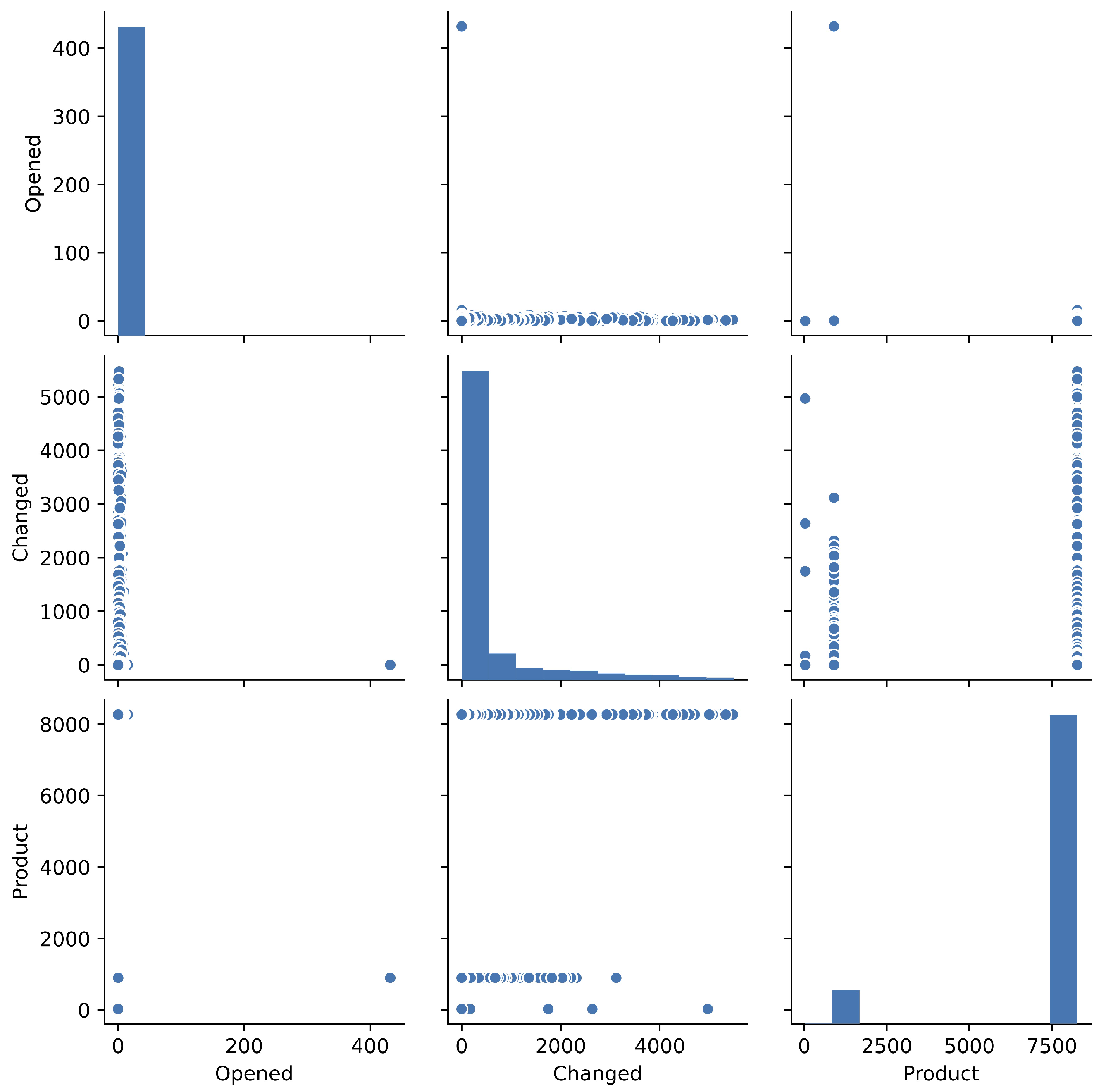
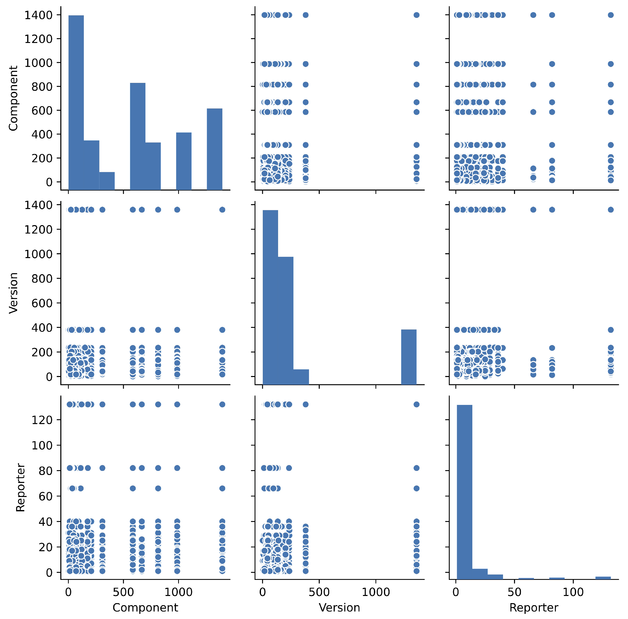
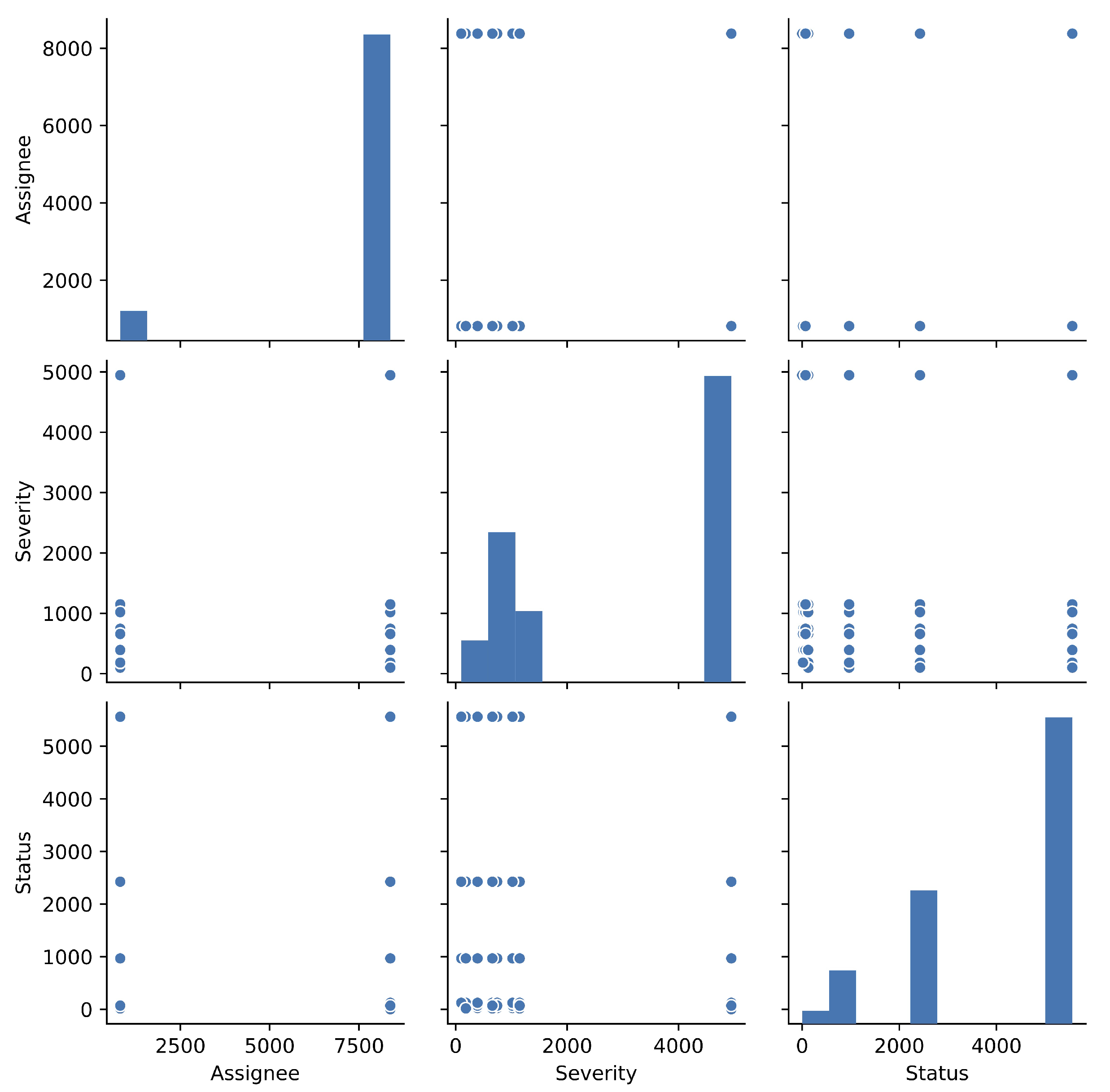
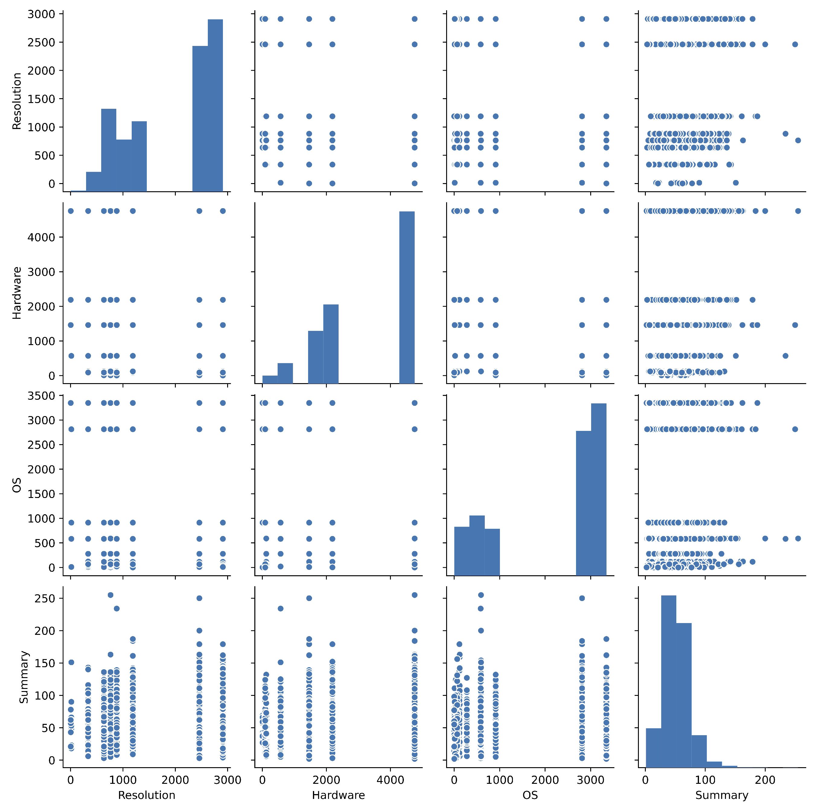
Generally, the number of data are used as the degree of freedom in the statistics. In the case of the big data, it is very difficult to estimate the upper and lower limits from the number of big data in the stochastic models, because the volume of data is huge. Many methods of OSS empirical assessment have been proposed [4,5,14,15]. However, the size of fault data in OSS is large. Therefore, it is difficult to assess the fault big data. Then, we focus on the number of explanatory variables. We will be able to estimate the upper and lower bounds by using the number of explanatory variables as the degree of freedom. The multiple regression analysis is well-known as the analysis method understanding the relationship between the objective variable and explanatory one. The analysis step in this paper is shown as follows:
Step 1:
The pairplots for each factor are used in order to overlooking the fault big data.
Step 2:
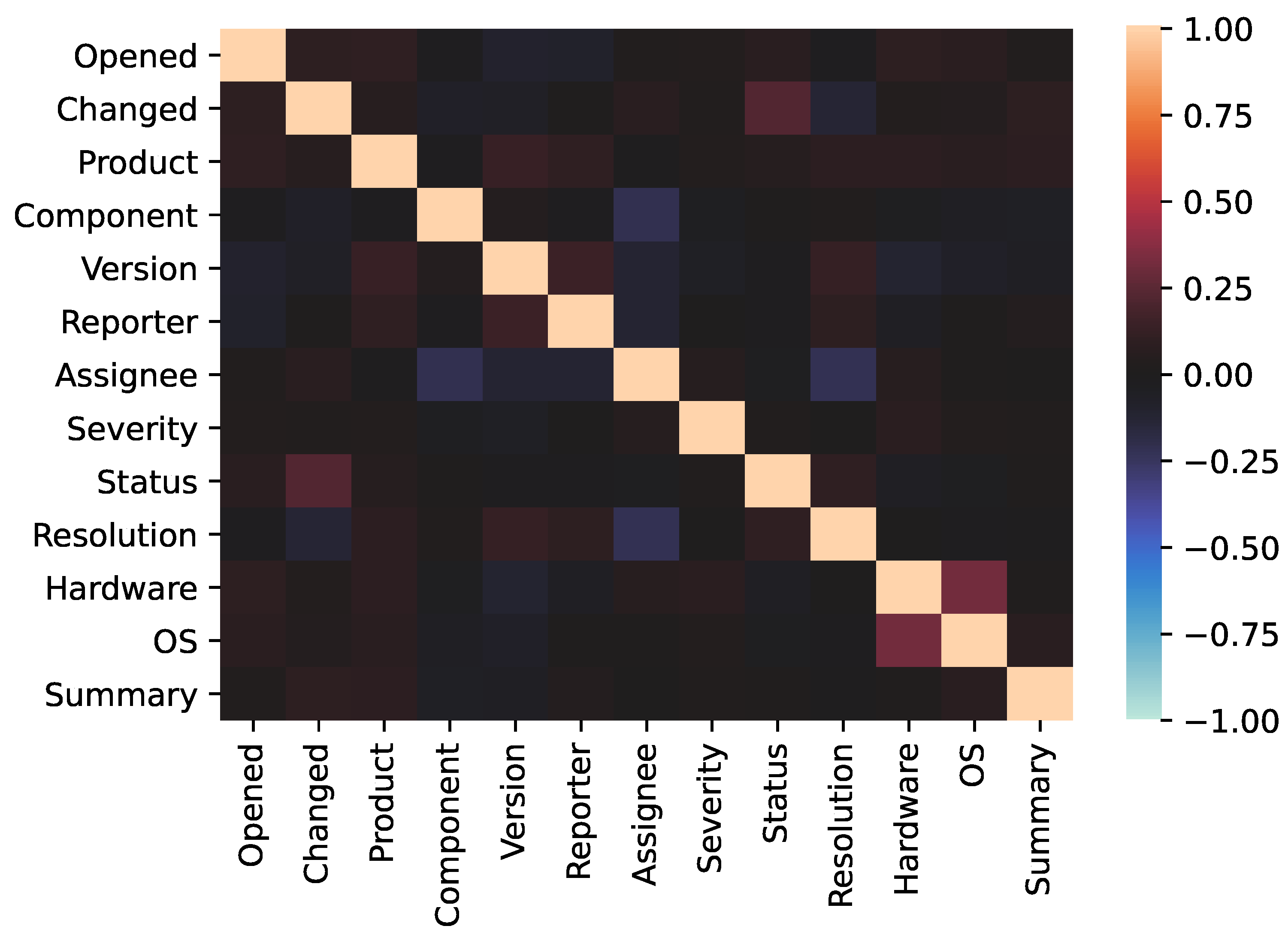
We apply the heatmap to the decision of the objective variable
Step 3:
The explanatory variables are narrowed by using the forward-backward stepwise selection method. Then, the degree of freedom is decided by the number of explanatory variables.
Step 4:
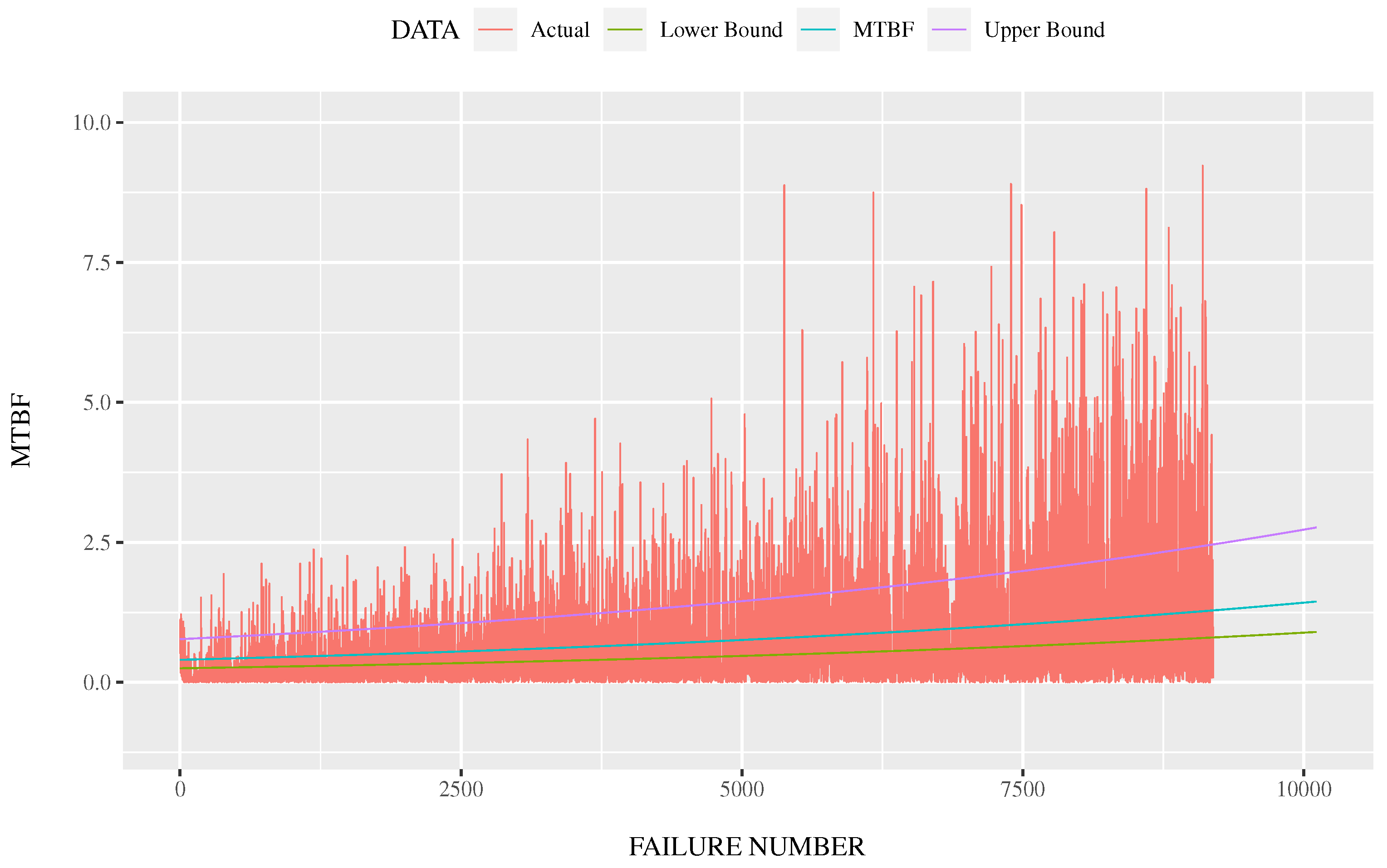
The upper and lower bounds are estimated from the stochastic model and the degree of freedom in place of the number of explanatory variables.
We show analysis examples by using the Apache HTTP Server Project [16] as the OSS. At first, we show the pairplot for the OSS fault big data in Figure 1, Figure 2, Figure 3 and Figure 4. We show the explanatory variables as follows:
Opened:The date and time recorded on the bug tracking system,
Changed:The modified date and time.
Product:The name of product included in OSS.
Component:The name of component included in OSS.
Version:The version number of OSS.
Reporter:The nickname of fault reporter.
Assignee:The nickname of fault assignee.
Severity:The level of fault.
Status:The fixing status of fault.
Resolution:The status of resolution of fault.
Hardware:The name of hardware under fault occurrence.
OS:The name of operating system under fault occurrence.
Summary:The brief contents of fault.
The set of 10,000 lines data are plotted in Figure 1, Figure 2, Figure 3 and Figure 4, respectively. Figure 1, Figure 2, Figure 3 and Figure 4 simply visualize the whole data. We can understand the whole trend of data from Figure 1, Figure 2, Figure 3 and Figure 4. Then, the number of whole data is about 130,000 data sets. In addition, all categories are simply shown by using three figures every three categories because of the convenience for the paper size.
Generally, the equation of multiple regression is given as follows:
F = β + α 1 x 1 + α 2 x 2 + α n x n ,
where F is the objective variable, α i i-th partial regression coefficient, and x i ( i = 1 , 2 , , n ) is i-th explanatory variable. β is the intercept.
Deciding the objective variable, we discuss the estimation results by the heatmap analysis. Then, the heatmap for actual fault big data is shown in Figure 5. From Figure 5, we find that the weight parameters of “Hardware”, “OS”, “Changed”, and “Status”are large. Therefore, we focus on 4 factors of “Hardware”, “OS”, “Changed”, and “Status” - as the objective variable, respectively. We analyze the data in the period from January 2001 to May 2020. The x and y axes of Figure 1, Figure 2, Figure 3, Figure 4 and Figure 5 are analyzed by using the values of Table 2.
Moreover, we analyze all categories of OSS fault big data by the multiple regression. The estimation results based on multiple regression analysis in cases of Hardware, OS, Changed, and Status as objective variables is shown in Table 3. For example, the top of Table 3 denotes that the objective variable is Hardware. Then, the other categories denote the explanatory variables. From Table 3, the multivariate regression models are obtained as follows:
(2) F h a r d w a r e = 1645.7 + 2.791757 x 1 0.067763 x 2 + 0.051574 x 3 0.008983 x 4 0.131288 x 5 0.146627 x 6 + 0.058349 x 7 + 0.063834 x 8 0.02625 x 9 + 0.003068 x 10 + 0.342187 x 11 0.452142 x 12 , (3) F o s = 1765.5 + 0.546647 x 1 0.042945 x 2 + 0.020329 x 3 0.072043 x 4 + 0.162994 x 5 + 0.040314 x 6 0.035459 x 7 0.010353 x 8 0.038089 x 9 0.028639 x 10 + 0.199227 x 11 + 3.442676 x 12 , (4) F c h a n g e d = 159.3 + 0.43598 x 1 + 0.027367 x 2 0.093938 x 3 0.054772 x 4 + 0.53278 x 5 + 0.019791 x 6 0.003285 x 7 + 0.120565 x 8 0.282455 x 9 0.024331 x 10 + 0.026484 x 11 + 1.344123 x 12 , (5) F s t a t u s = 3191.5 1.334526 x 1 + 0.444458 x 2 + 0.030289 x 3 + 0.069858 x 4 0.197055 x 5 + 0.366868 x 6 0.018191 x 7 + 0.025926 x 8 + 0.423487 x 9 0.034746 x 10 0.086595 x 11 + 1.250057 x 12 .

4. Forward-Backward Stepwise Selection Method

The forward-backward stepwise selection method is well-known as the selection method of explanatory variables for the multiple regression analysis. We use the forward-backward stepwise selection method as the multiple regression analysis for OSS fault big data. The forward-backward stepwise selection method is well-known as the selection method of explanatory variables in multiple regression analysis. In particular, we apply the backward stepwise selection method. Then, we consider the following steps:
Step 1:
All explanatory variables are analyzed by the multiple regression.
Step 2:
As the results of step 1, the explanatory variable is removed if p-value becomes large than 0.01.
Step 3:
The selected explanatory variables are analyzed by the multiple regression again.
Step 4:
The above steps 1 and 2 are continued until there is no p-value of explanatory variable larger than 0.01.
There are many methods as forward-backward stepwise selection ones. Then, it will be difficult to analyze the fault big data sets by using the other complex analysis method. Therefore, this paper is simply analyzed by above steps, because the fault big data sets have many factors and lines of bugs. In the case of the big data, it is very important to consider the calculation time and complexity in the estimation.
From Table 4, the multivariate regression models based on backward stepwise selection method are obtained as follows:
(6) F h a r d w a r e = 1626.4 0.068803 x 1 + 0.05123 x 2 0.130621 x 3 + 0.058414 x 4 + 0.063954 x 5 0.026041 x 6 + 0.341771 x 7 , (7) F o s = 1743.1 + 0.043135 x 1 + 0.020108 x 2 0.071013 x 3 + 0.163322 x 4 0.035639 x 5 0.038459 x 6 0.028896 x 7 + 0.198147 x 8 + 3.431072 x 9 , (8) F c h a n g e d = 156.8 + 0.027344 x 1 0.09417 x 2 0.051485 x 3 + 0.019413 x 4 + 0.120492 x 5 0.282509 x 6 0.024697 x 7 + 0.026598 x 8 + 1.348889 x 9 , (9) F s t a t u s = 3316.2 + 0.444006 x 1 + 0.03109 x 2 0.198328 x 3 0.021023 x 4 + 0.025704 x 5 + 0.422041 x 6 0.034968 x 7 0.086049 x 8 .
In particular, the selection results from explanatory variable is shown in Table 5 by using the method of backward stepwise selection. From Table 5, “Product”, “Version”, and “Assignee”are included as the common factors for all objective variables. This means that these three factors are very important factors to detect and fix the fault recorded on the bug tracking system. From this estimation results, we consider that the OSS developers can appropriately manage by using the information obtained from “Product”, “Version”, and “Assignee”. On the other hand, “Opened” and “Reporter” have been removed from all explanatory variables by using the backward stepwise selection method. In other words, “Opened” and “Reporter” may not be important from the standpoint of the quality control of OSS.

5. Multiple Regression Analysis with Application to Reliability Assessment

Many software reliability assessment models have been proposed in the past [17,18,19,20,21]. In particular, the hazard rate model is well-known as the typical software reliability model. We apply the hazard rate model to the time-interval between correction faults. The distribution function of X k ( k = 1 , 2 , ) representing the time-interval between correction faults of ( k 1 ) th and k-th is defined as:
Q k ( x ) Pr { X k x } ( x 0 ) ,
where Pr { Φ } represents the occurrence probability event Φ . Therefore, the following derived function means the probability density function of X k :
q k ( x ) d Q k ( x ) d x .
From Equations (10) and (11), the hazard rate is given by the following equation:
z k ( x ) q k ( x ) 1 Q k ( x ) ,
where the hazard rate means [1,22] the software correction rate when the software correction does not occur during the time-interval ( 0 , x ] . Therefore, the software reliability assessment measures are obtained from the typical hazard rate model in Equation (12). The probability density function can be derived as
z k ( x ) = ϕ ( N k + 1 ) ,
where N is the number of latent faults in OSS, ϕ the hazard rate per inherent fault. Then, the mean time between software failures correction ( M T B F c ) is given as follows:
E [ X k ] = 0 x q k ( x ) d x = 0 1 Q k ( x ) d x = 0 e ϕ ( N k + 1 ) x d x = e ϕ ( N k + 1 ) x ϕ ( N k + 1 ) 0 = 1 ϕ ( N k + 1 ) .
It is important to assess the upper and lower bounds of M T B F c , E [ X k ] , because the difficulty of fault correction continuously keeps the variation state. Then, the upper and lower confidence limits for the M T B F c can be estimated from Chi-squared distribution. Then, the upper and lower confidence limits in 100 ( 1 α ) percentage point of Chi-squared distribution for the M T B F c is given by
2 m E ^ [ X k ] χ 2 m 2 ( α 2 ) E ^ [ X k ] 2 m E ^ [ X k ] χ 2 m 2 ( 1 α 2 ) ,
where m is the statistical degrees of freedom in objective variable of the regression equation. Then, we consider the regression equation of Equation (8). The explanatory variables are shown in Table 4. From Equation (8) and Table 4, the statistical degrees of freedom for the regression equation is 9 in the case of “Changed”. In the case of “Changed”, 90 % upper and lower confidence limits for M T B F c are as follows:
18 E ^ [ X k ] χ 18 2 ( 0.1 2 ) E ^ [ X k ] 18 E ^ [ X k ] χ 18 2 ( 1 0.1 2 ) .
As an example, the estimated upper and lower confidence limits for M T B F c are shown in Figure 6. As shown in Figure 6, we can assess the upper and lower confidence limits for M T B F c . By using the estimation results in Equation (8) and Table 4, we can consider the influence degrees from the explanatory variables for M T B F c as the upper and lower confidence limits. The upper and lower bounds in Figure 6 mean the influences from “Product”, “Component”, “Version”, “Assignee”, “Status”, “Resolution”, “Hardware”, “OS”, and “Summary”as the main factors.
Several research papers have proposed the methods in terms of the upper and lower limits based on software reliability growth models, and the empirical approach for OSS [23,24]. As the comparison with the conventional method, we show the estimated upper and lower confidence limits based on the conventional method in Figure 7. The number of fault data is used as the degree of freedom in Figure 7. In Figure 7, we found that the conventional method can not estimate the upper and lower bounds accurately because the value of degree of freedom is large. On the other hand, the proposed method can appropriately estimate the upper and lower confidence limits for the actual fault big data, because the degree of freedom is properly given by using the proposed method.
As the comparison results of the other model, we compare the following Moranda model with the Jelinski–Moranda model.
E [ X k ] = 1 D ( c k 1 ) .
where c is the decreasing rate of hazard rate, D the hazard rate per inherent fault.
Similarly, we show the estimated upper and lower confidence limits for the M T B F c in actual fault big data in the case of the Moranda model in Figure 8. Moreover, we show the estimated upper and lower confidence limits based on the conventional method in the case of the Moranda model in Figure 9.
As our main contribution, we have proposed the estimation method for upper and lower confidence limits based on the typical hazard rate model. The conventional models cannot estimate the upper and lower confidence limits because the degree of freedom is very large. The proposed method can estimate the upper and lower confidence limits based on the typical hazard rate model in case of large scale fault data sets by using our method.

6. Conclusions

We have discussed the quantification method of the first type for the fault recorded on the bug tracking system of OSS. Then, we apply the multiple regression analysis. We have found that the proposed method can assess the important factors in terms of the OSS quality control by using the multiple regression analysis.
It is difficult for the OSS developers to assess from the bug tracking system because the fault big data are large scale. The proposed method is simple structure by using the traditional stepwise selection method. Therefore, our method can be simply use for the other OSS. The proposed method can find the main factors as explanatory variables affecting the quality management. Thereby, the OSS developer will be able to easily assess the quality from the standpoint of the condition recorded from actual fault big data.
In particular, we have applied the estimation results of multiple regression analysis to the reliability assessment. Under the situation of big data, the objective variable will depend on various explanatory variables. We have proposed the reliability assessment method based on the multiple regression analysis and stochastic model for the OSS fault big data. As the study, the OSS managers can assess the upper and lower limits of the software reliability models for the fault big data. Thereby, the OSS managers can comprehend the stability of OSS development and operation.

Author Contributions

Conceptualization, Y.T.; Methodology, Y.T.; Validation, Y.T. and S.Y.; Formal Analysis, Y.T.; Data Curation, Y.T.; Visualization, Y.T.; Project Administration, Y.T. and S.Y. All authors have read and agreed to the published version of the manuscript.

Funding

This research was funded by the JSPS KAKENHI Grant No.20K11799 in Japan. Thank JSPS KAKEN HI Grant No. 20K11799 in Japan for supporting this work.

Conflicts of Interest

The authors declare no conflict of interest.

References

  1. Yamada, S. Software Reliability Modeling: Fundamentals and Applications; Springer: Tokyo, Japan; Heidelberg, Germany, 2014. [Google Scholar]
  2. Kapur, P.K.; Pham, H.; Gupta, A.; Jha, P.C. Software Reliability Assessment with OR Applications; Springer: London, UK, 2011. [Google Scholar]
  3. Yamada, S.; Tamura, Y. OSS Reliability Measurement and Assessment; Springer International Publishing: Basel, Switzerland, 2016. [Google Scholar]
  4. Zhou, Y.; Davis, J. Open source software reliability model: An empirical approach. In Proceedings of the Fifth Workshop on Open Source Software Engineering (5-WOSSE), St Louis, MO, USA, 17 May 2005; pp. 1–6. [Google Scholar] [CrossRef]
  5. Norris, J. Mission-critical development with open source software. IEEE Softw. Mag. 2004, 21, 42–49. [Google Scholar] [CrossRef]
  6. Janczarek, P.; Sosnowski, J. Investigating software testing and maintenance reports: Case study. Inf. Softw. Technol. 2015, 58, 272–288. [Google Scholar] [CrossRef]
  7. Li, Q.; Pham, H. A Generalized Software Reliability Growth Model With Consideration of the Uncertainty of Operating Environments. IEEE Access 2019, 7, 84253–84267. [Google Scholar] [CrossRef]
  8. Tariq, I.; Maqsood, T.B.; Hayat, B.; Hameed, K.; Nasir, M.; Jahangir, M. The comprehensive study on software reliability. In Proceedings of the 2018 International Conference on Computing, Mathematics and Engineering Technologies (iCoMET), Sukkur, Pakistan, 3–4 March 2018; pp. 1–7. [Google Scholar]
  9. Korpalski, M.; Sosnowski, J. Correlating software metrics with software defects. In Proceedings of the Photonics Applications in Astronomy, Communications, Industry, and High-Energy Physics Experiments, Wilga, Poland, 27 May–5 June 2018. [Google Scholar] [CrossRef]
  10. Madeyski, L.; Jureczko, M. Which process metrics can significantly improve defect prediction models? An empirical study. Softw. Qual. J. 2015, 23, 393–422. [Google Scholar] [CrossRef] [Green Version]
  11. Park, N.J.; George, K.M.; Park, N. A multiple regression model for trend change prediction. In Proceedings of the 2010 International Conference on Financial Theory and Engineering, Dubai, UAE, 18–20 June 2010; pp. 22–26. [Google Scholar] [CrossRef]
  12. Aiyin, W.; Yanmei, X. Multiple Linear Regression Analysis of Real Estate Price. In Proceedings of the 2018 International Conference on Robots & Intelligent System (ICRIS), Changsha, China, 26–27 May 2018; pp. 564–568. [Google Scholar] [CrossRef]
  13. Rahil, A.; Mbarek, N.; Togni, O.; Atieh, M.; Fouladkar, A. Statistical learning and multiple linear regression model for network selection using MIH. In Proceedings of the Third International Conference on e-Technologies and Networks for Development (ICeND2014), Beirut, Lebanon, 29 April–1 May 2014; pp. 189–194. [Google Scholar] [CrossRef]
  14. Singh, V.B.; Sharma, M.; Pham, H. Entropy based software reliability analysis of multi-version open source software. IEEE Trans. Softw. Eng. 2017. [Google Scholar] [CrossRef]
  15. Lavazza, L.; Morasca, S.; Taibi, D.; Tosi, D. An empirical investigation of perceived reliability of open source Java programs. In Proceedings of the 27th Annual ACM Symposium on Applied Computing (SAC ’12), Trento, Italy, 26–30 March 2012; pp. 1109–1114. [Google Scholar] [CrossRef]
  16. The Apache Software Foundation, The Apache HTTP Server Project. Available online: http://httpd.apache.org/ (accessed on 14 October 2020).
  17. Tamura, Y.; Yamada, S. Dependability analysis tool based on multi-dimensional stochastic noisy model for cloud computing with big data. Int. J. Math. Eng. Manag. Sci. 2017, 2, 273–287. [Google Scholar] [CrossRef]
  18. Tamura, Y.; Yamada, S. Open source software cost analysis with fault severity levels based on stochastic differential equation models. J. Life Cycle Reliab. Saf. Eng. 2017, 6, 31–35. [Google Scholar] [CrossRef]
  19. Tamura, Y.; Yamada, S. Dependability analysis tool considering the optimal data partitioning in a mobile cloud. In Reliability Modeling with Computer and Maintenance Applications; World Scientific: Singapore, 2017; pp. 45–60. [Google Scholar]
  20. Tamura, Y.; Yamada, S. Multi-dimensional software tool for OSS project management considering cloud with big data. Int. J. Reliab. Qual. Saf. Eng. 2018, 25, 1850014-1–1850014-16. [Google Scholar] [CrossRef]
  21. Tamura, Y.; Yamada, S. Maintenance effort management based on double jump diffusion model for OSS project. Ann. Oper. Res. 2019, 1–16. [Google Scholar] [CrossRef]
  22. Jelinski, Z.; Moranda, P.B. Software Reliability Research, in Statistical Computer Performance Evaluation; Freiberger, W., Ed.; Academic Press: New York, NY, USA, 1972; pp. 465–484. [Google Scholar]
  23. Yin, L.; Trivedi, K.S. Confidence interval estimation of NHPP-based software reliability models. In Proceedings of the 10th International Symposium on Software Reliability Engineering (Cat. No.PR00443), Boca Raton, FL, USA, 1–4 November 1999; pp. 6–11. [Google Scholar] [CrossRef]
  24. Okamura, H.; Grottke, M.; Dohi, T.; Trivedi, K.S. Variational Bayesian Approach for Interval Estimation of NHPP-Based Software Reliability Models. In Proceedings of the 37th Annual IEEE/IFIP International Conference on Dependable Systems and Networks (DSN’07), Edinburgh, UK, 25–28 June 2007; pp. 698–707. [Google Scholar] [CrossRef]
Figure 1. The pairplot for actual fault big data (1).
Make 02 00024 g001
Figure 2. The pairplot for actual fault big data (2).
Make 02 00024 g002
Figure 3. The pairplot for actual fault big data (3).
Make 02 00024 g003
Figure 4. The pairplot for actual fault big data (4).
Make 02 00024 g004
Figure 5. The heatmap for actual fault big data.
Make 02 00024 g005
Figure 6. The estimated upper and lower confidence limits for the M T B F c in actual fault big data.
Make 02 00024 g006
Figure 7. The estimated upper and lower confidence limits based on the conventional method.
Make 02 00024 g007
Figure 8. The estimated upper and lower confidence limits for the M T B F c in actual fault big data in the case of the Moranda model.
Make 02 00024 g008
Figure 9. The estimated upper and lower confidence limits based on the conventional method in the case of the Moranda model.
Make 02 00024 g009
Table 1. A part of the raw fault big data.
OpenedProductComponentVersionReporterAssignee
0.83895Apache httpd-1.3Documentation1.3.23rineau+apachebugzilladocs
1.12118Apache httpd-1.3Other mods1.3.24siegfried.delwichebugs
0.17191Apache httpd-1.3Documentation1.3.23dardbugs
0.40766Apache httpd-1.3Other1.3.23bernard.l.dubreuildocs
0.51352Apache httpd-1.3Other1.3.23georgebugs
SeverityStatusResolutionHardwareOS
normalCLOSEDFIXEDOtherother
blockerCLOSEDFIXEDPCLinux
normalCLOSEDFIXEDAllFreeBSD
minorCLOSEDFIXEDAllAll
normalCLOSEDWORKSFORMEPCLinux
Table 2. A part of the numerical value converted from the raw fault big data.
OpenedProductComponentVersionReporterAssignee
0.83895898815951815
1.12118898916218378
0.171918988159518378
0.40766898141952815
0.513528981419518378
SeverityStatusResolutionHardwareOS
4946242629101460912
3922426291047553347
4946242629102188278
6582426291021882812
4946242633547553347
Table 3. The estimation results in cases Hardware, OS, Changed, and Status as objective variables.
HardwareEstimateStd. Errort Valuep Value
Intercept1645.720058114.70012714.3480
Opened2.7917573.4986860.79790.424923
Changed−0.0677630.017142−3.95310.000078
Product0.0515740.0054919.39330
Component−0.0089830.032654−0.27510.783246
Version−0.1312880.037497−3.50130.000465
Reporter−0.1466270.873514−0.16790.866698
Assignee0.0583490.00503511.58880
Severity0.0638340.007538.47760
Status−0.026250.008096−3.24240.00119
Resolution0.0030680.0168160.18240.855249
OS0.3421870.01237827.64390
Summary−0.4521420.712837−0.63430.525911
OSEstimateStd. Errort ValuepValue
Intercept1765.50600186.55717420.3970
Opened0.5466472.6697270.20480.837766
Changed0.0429450.0130783.28370.001028
Product0.0203290.0042114.82770.000001
Component−0.0720430.024922−2.89080.003852
Version0.1629940.0285145.71620
Reporter0.0403140.6664620.06050.951767
Assignee−0.0354590.003937−9.00610
Severity−0.0103530.005781−1.79080.073361
Status−0.0380890.006183−6.16030
Resolution−0.0286390.012835−2.23140.02568
Hardware0.1992270.00726127.43810
Summary3.4426760.5394526.38180
ChangedEstimateStd. Errort ValuepValue
Intercept159.27464769.475372.29250.021897
Opened0.435982.0966360.20790.835278
Product0.0273670.0033668.12950
Component−0.0939380.019572−4.79960.000002
Version−0.0547720.022467−2.43790.014792
Reporter0.532780.5233981.01790.30874
Assignee0.0197910.0031216.34110
Severity−0.0032850.004545−0.72270.469904
Status0.1205650.00478225.21410
Resolution−0.2824550.009813−28.78290
Hardware−0.0243310.005928−4.10440.000041
OS0.0264840.0077563.41460.000642
Summary1.3441230.4271393.14680.001656
StatusEstimateStd. Errort ValuepValue
Intercept3191.460936129.21312824.69920
Opened−1.3345264.025544−0.33150.740264
Changed0.4444580.01922423.11960
Product0.0302890.0062154.87370.000001
Component0.0698580.0374011.86780.061817
Version−0.1970550.043141−4.56770.000005
Reporter0.3668681.0047870.36510.715031
Assignee−0.0181910.005768−3.1540.001616
Severity0.0259260.0086742.98890.002807
Resolution0.4234870.01839123.02640
Hardware−0.0347460.011364−3.05760.002238
OS−0.0865950.014885−5.81760
Summary1.2500570.8169141.53020.125997
Table 4. The estimation results by backward stepwise selection method in cases Hardware, OS, Changed, and Status as objective variables.
HardwareEstimateStd. Errort Valuep Value
Intercept1626.40521997.4396316.69140
Changed−0.0688030.016619−4.14010.000035
Product0.051230.005329.62920
Version−0.1306210.037285−3.50330.000462
Assignee0.0584140.00498911.70870
Severity0.0639540.0075038.52330
Status−0.0260410.007774−3.34980.000812
OS0.3417710.01231527.75240
OSEstimateStd. Errort ValuepValue
Intercept1743.08585485.25001820.44680
Changed0.0431350.013083.29780.000978
Product0.0201080.0041394.85860.000001
Component−0.0710130.024916−2.85010.00438
Version0.1633220.0284855.73360
Assignee−0.0356390.00385−9.25730
Status−0.0384590.006145−6.25870
Resolution−0.0288960.012789−2.25950.023879
Hardware0.1981470.00719227.55050
Summary3.4310720.5379226.37840
ChangedEstimateStd. Errort ValuepValue
Intercept156.81089368.428012.29160.02195
Product0.0273440.0033148.25220
Component−0.094170.019566−4.81290.000002
Version−0.0514850.022444−2.29390.021816
Assignee0.0194130.0030566.3530
Status0.1204920.00475225.35390
Resolution−0.2825090.009778−28.89230
Hardware−0.0246970.00588−4.20010.000027
OS0.0265980.0077483.43270.0006
Summary1.3488890.4259983.16640.001548
StatusEstimateStd. Errort ValuepValue
Intercept3316.187141116.4920928.46710
Changed0.4440060.01922623.09430
Product0.031090.0061815.03030
Version−0.1983280.043107−4.60080.000004
Assignee−0.0210230.005759−3.65020.000263
Severity0.0257040.0086732.96370.003048
Resolution0.4220410.01828523.08150
Hardware−0.0349680.011359−3.07840.002087
OS−0.0860490.014875−5.78460
Table 5. The selection results of explanatory variable.
Factors Selected from
All Objective Variables
Factors Removed from
All Objective Variables
ProductOpened
VersionReporter
Assignee———–
Publisher’s Note: MDPI stays neutral with regard to jurisdictional claims in published maps and institutional affiliations.

