Figure 1.
Study site land use (NLCD 2011), Soil & Climate Analysis Network (SCAN) stations (orange), and elevation profile (purple) for (clockwise from top left) Elk river watershed (ELKR), Yazoo (YAZO), Washita (WASH), and Escalante-Sevier Lake (ESCL). The red curves outline each basin.
Figure 1.
Study site land use (NLCD 2011), Soil & Climate Analysis Network (SCAN) stations (orange), and elevation profile (purple) for (clockwise from top left) Elk river watershed (ELKR), Yazoo (YAZO), Washita (WASH), and Escalante-Sevier Lake (ESCL). The red curves outline each basin.
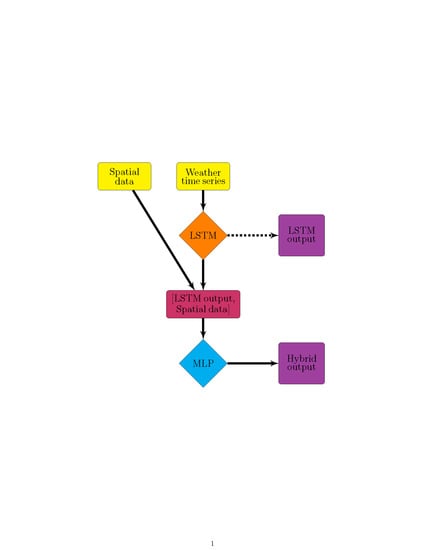
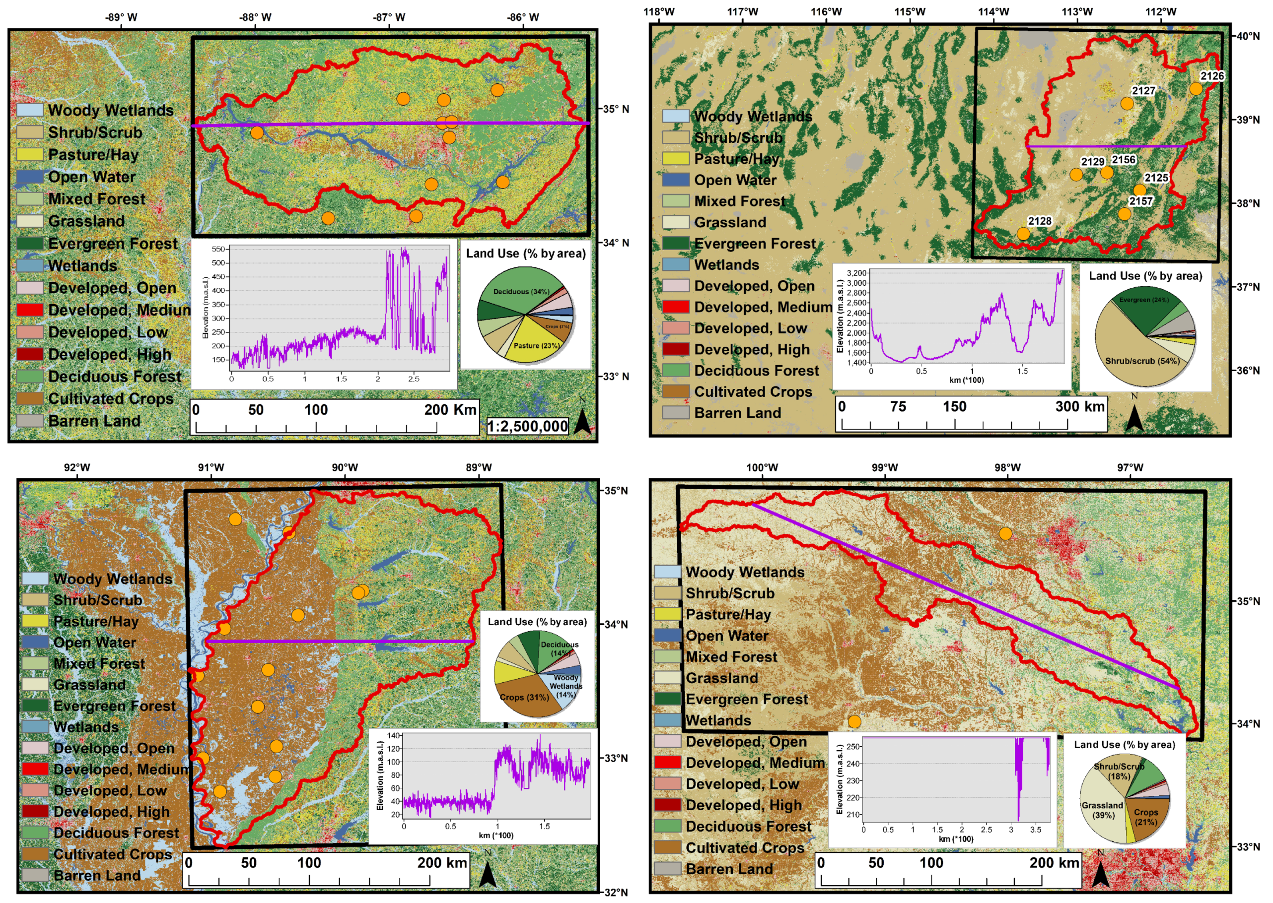
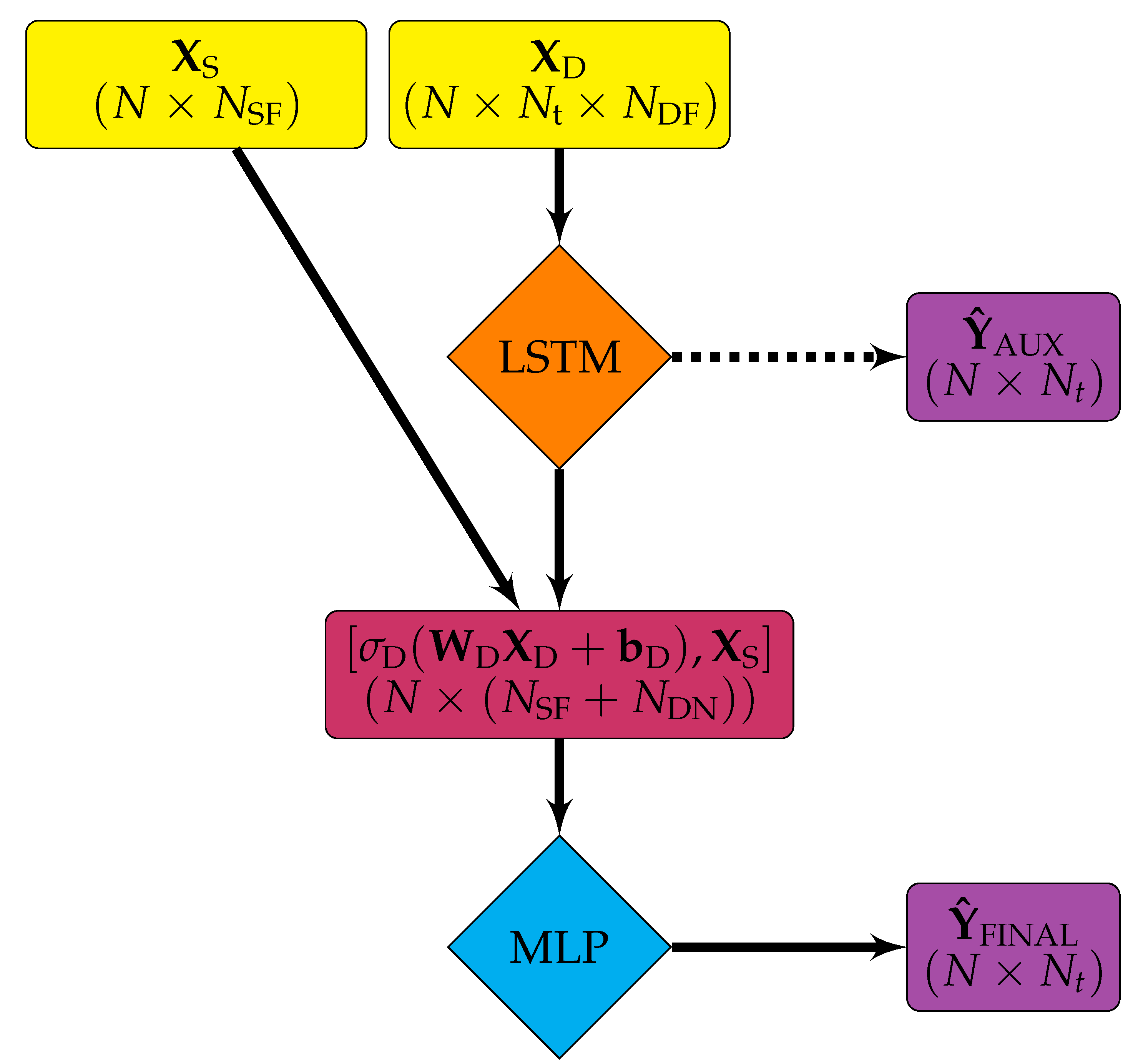
Figure 2.
Hybrid architecture where is the three-dimensional array of dynamic (time series) inputs, is the two-dimensional array of static inputs, N is the number of samples, is the number of time steps, is the number of dynamic features, is the number of static features, and is the number of nodes in the long short-term memory (LSTM) layers.
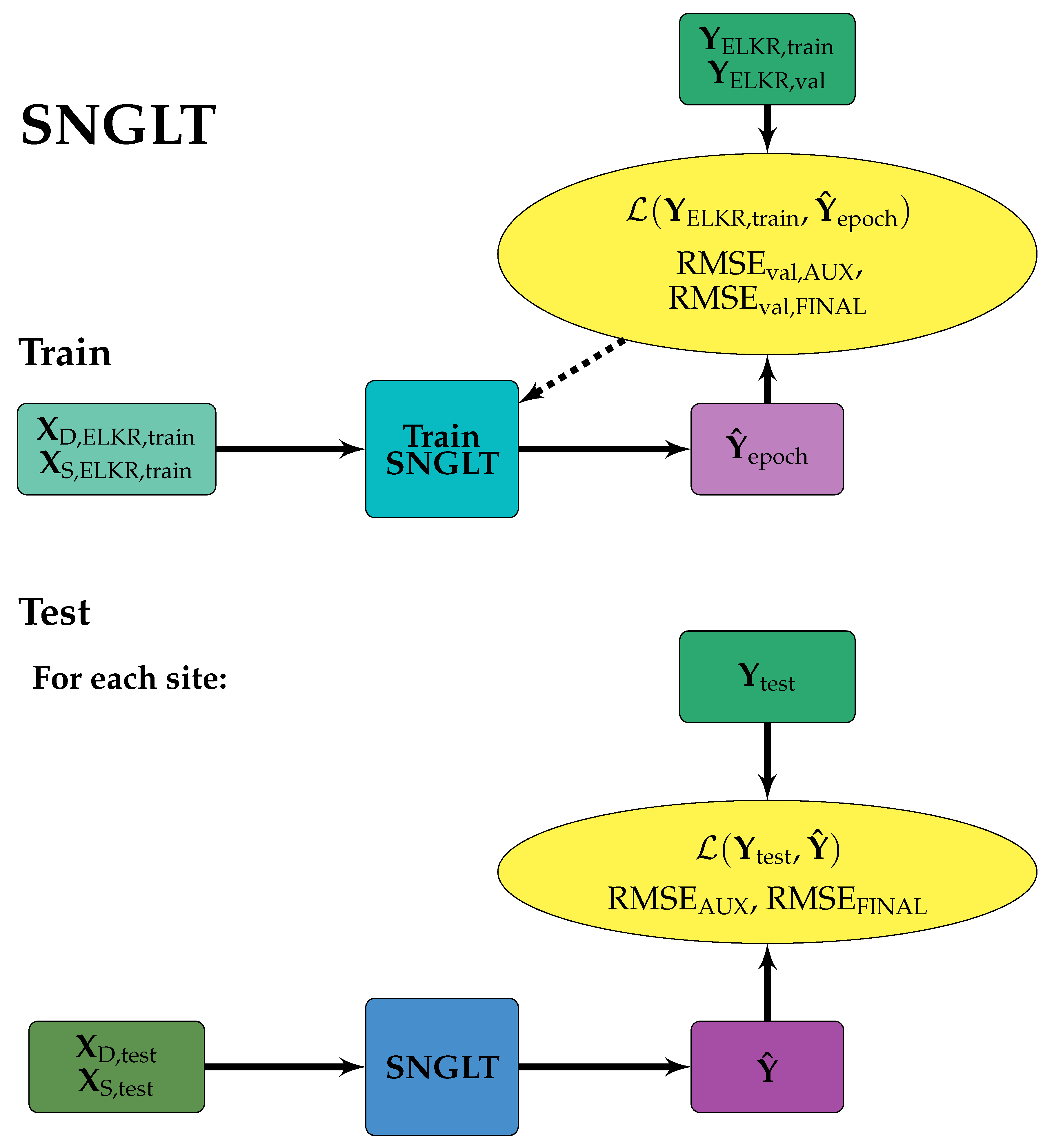
Figure 3.
SNGLT model design. Solid arrows indicate the forward flow of information, dashed arrows indicate information used to make updates to model weights and/or inform early stopping. Training data were from the ELKR site only. The trained model was then applied to each site individually.
Figure 3.
SNGLT model design. Solid arrows indicate the forward flow of information, dashed arrows indicate information used to make updates to model weights and/or inform early stopping. Training data were from the ELKR site only. The trained model was then applied to each site individually.
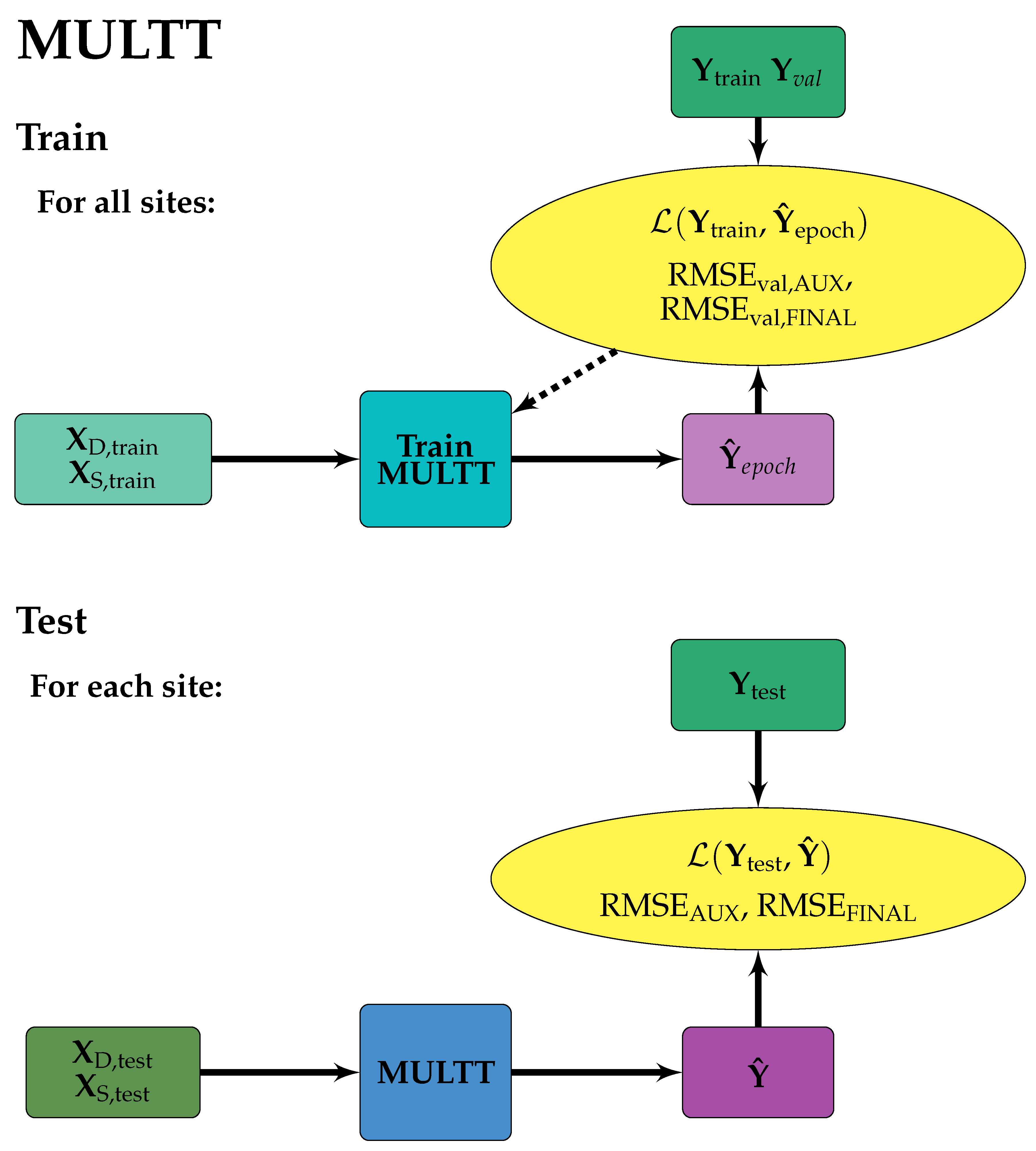
Figure 4.
MULTT model design. Solid arrows indicate the forward flow of information, dashed arrows indicate information used to make updates to model weights and/or inform early stopping. Training data were from all sites, such that each tensor was a concatenation of training data from each site along the samples axis. The trained model was then applied to each site individually.
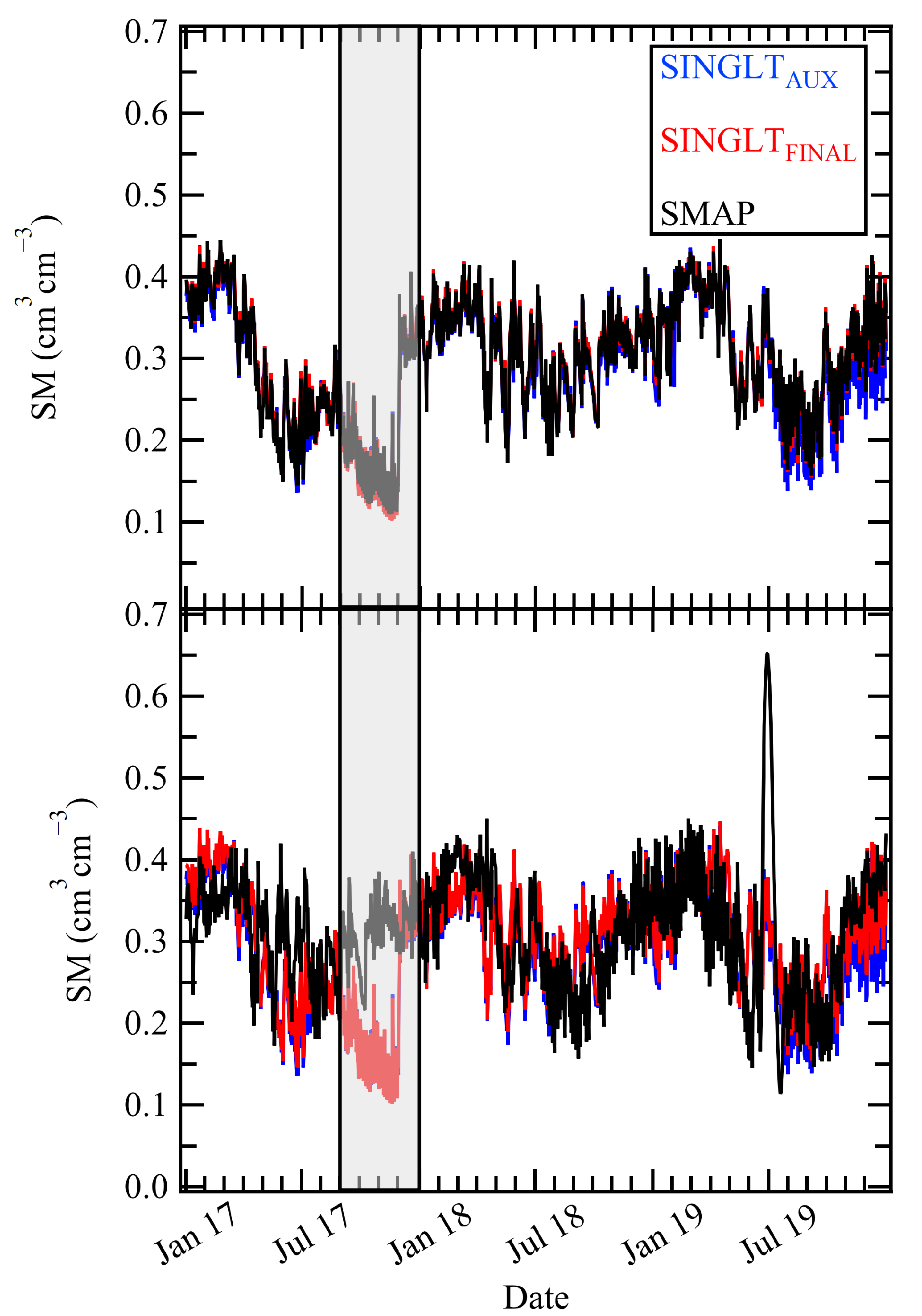
Figure 5.
SNGLT_PGLNF model results for the ELKR site during the TIME_E (top) and TIME_P (bottom) periods. Results shown are for the SNGLT model evaluated on the ELKR test set. The gray box shows a severe drought observed in the late summer and fall of 2016 that was falsely predicted during the TIME_P period, indicating overfitting to the training data.
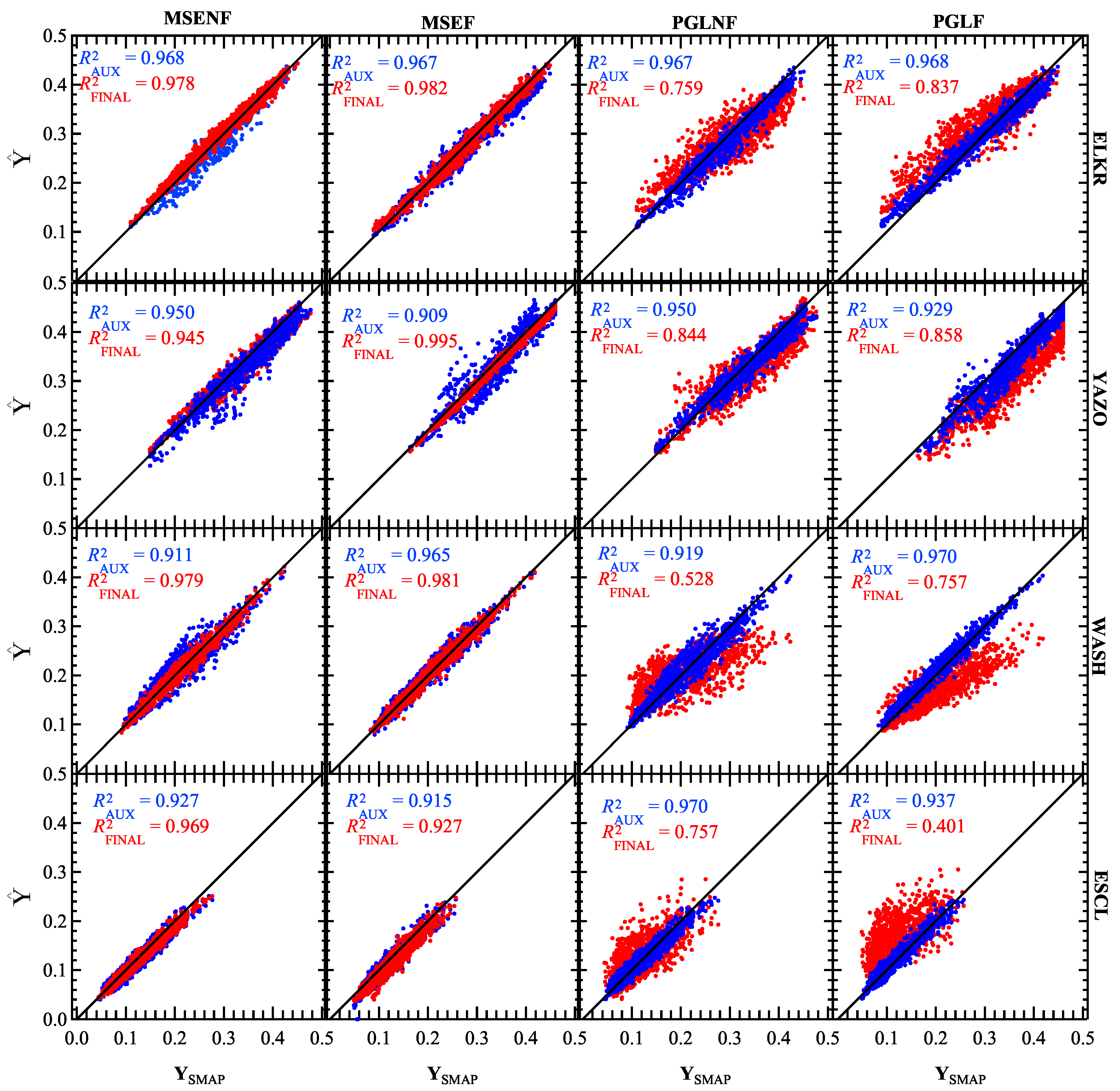
Figure 6.
Results for MULTT experiments trained and tested on all four watersheds during the TIME_E period (1 January 2016–31 December 2018). The rows show results for each study site (from top): ELKR, YAZO, WASH, ESCL. The columns are (from left): MULTT_MSENF, MULTT_MSEF, MULTT_PGLNF, MULTT_PGLF. Results for vs. are shown in blue, and vs. are shown in red. The output with the highest accuracy is shown as the top layer in each subplot, highlighting the effectiveness of each loss function.
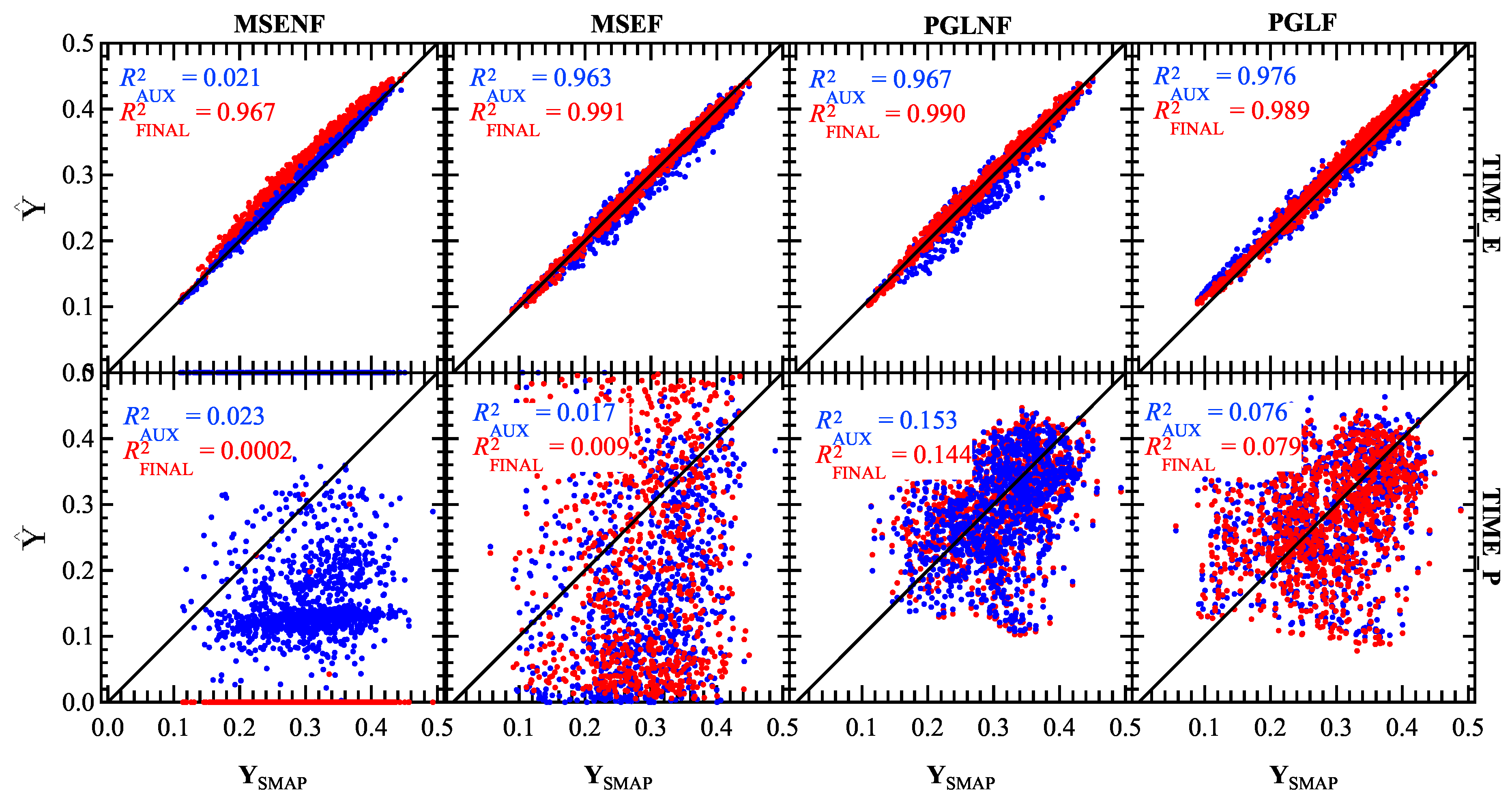
Figure 7.
ELKR model results from the AUX (blue) and FINAL (red) outputs plotted vs. SMAP SM labels. Results are shown for the trained SNGLT model applied to ELKR test sets for the TIME_E (top; 1 January 2016–31 December 2018) and TIME_E (bottom; 1 January 2017–31 December 2019) time periods. Results are shown for all experiments (from left) SNGLT_MSENF, SNGLT_MSEF, SNGLT_PGLNF, and SNGLT_PGLF. The output with the highest accuracy is shown as the top layer in each subplot, highlighting the effectiveness of each loss function.
Table 1.
Static parameters from Soil & Water Assessment Tool plus (SWAT+) hydrologic input datasets used as features for the multilayer perceptron (MLP) network.
Table 1.
Static parameters from Soil & Water Assessment Tool plus (SWAT+) hydrologic input datasets used as features for the multilayer perceptron (MLP) network.
| Parameter | Description | Type |
|---|
| CN2 | Curve number | Numerical |
| SOILDEP | Depth of soil profile | Numerical |
| SLOPE | Percent slope | Numerical |
| SLOPELEN | Length of sloping surface (m) | Numerical |
| ITEXT | Soil textural characteristics | Categorical |
| IPLANT | Land-use type | Categorical |
| USLEK | Soil erodibility factor | Numerical |
| USLEC | Crop/vegetation management factor | Numerical |
Table 2.
Weather-parameter feature vectors for the LSTM and their sources. Missing values from NOAA data were filled in using long-term monthly means and the SWAT+ weather generator.
Table 2.
Weather-parameter feature vectors for the LSTM and their sources. Missing values from NOAA data were filled in using long-term monthly means and the SWAT+ weather generator.
| Parameter | Source |
|---|
| Precipitation (mm) | NOAA ISD |
| Temperature (max, min, mean; °C) | NOAA ISD |
| Wind Speed (m/s) | NOAA ISD |
| Wind Direction (°) | NOAA ISD |
| Solar Radiation (mean, max; W m–2) | SWAT+ weather generator |
| Relative Humidity (kPa) | SWAT+ weather generator |
| Dewpoint (°C) | SWAT+ weather generator |
Table 3.
Definitions of feature and label vector with dimensions for the LSTM (dynamic) input (), MLP (static) input (), Soil Moisture Active Passive (SMAP) SM timeseries (), LSTM SM auxiliary estimate of (), LSTM-MLP final SM estimate of () for SNGLT and MULTT model designs.
Table 3.
Definitions of feature and label vector with dimensions for the LSTM (dynamic) input (), MLP (static) input (), Soil Moisture Active Passive (SMAP) SM timeseries (), LSTM SM auxiliary estimate of (), LSTM-MLP final SM estimate of () for SNGLT and MULTT model designs.
| Variable | Definition | Value |
|---|
| Number of time steps | 1096 |
| Number of dynamic features | 22 (without SAT flag) 44 (with SAT flags) |
| Number of static features | 56 |
Table 4.
Experimental design. Two model designs were trained and evaluated: (1) SNGLT was trained on the ELKR site only and tested on ELKR, YAZO, WASH, and ESCL sites individually and (2) MULTT was trained using data from all four sites at once, then evaluated on each site individually.
Table 4.
Experimental design. Two model designs were trained and evaluated: (1) SNGLT was trained on the ELKR site only and tested on ELKR, YAZO, WASH, and ESCL sites individually and (2) MULTT was trained using data from all four sites at once, then evaluated on each site individually.
| Model | Experiment | Training Sites | Loss Function | SAT Flags |
|---|
| SNGLT | SNGLT_MSENF | ELKR | MSE | No |
| SNGLT | SNGLT_MSEF | ELKR | MSE | Yes |
| SNGLT | SNGLT_PGLNF | ELKR | PGL | No |
| SNGLT | SNGLT_PGLF | ELKR | PGL | Yes |
| MULTT | MULTT_MSENF | ELKR, YAZO, WASH, ESCL | MSE | No |
| MULTT | MULTT_MSEF | ELKR, YAZO, WASH, ESCL | MSE | Yes |
| MULTT | MULTT_PGLNF | ELKR, YAZO, WASH, ESCL | PGL | No |
| MULTT | MULTT_PGLF | ELKR, YAZO, WASH, ESCL | PGL | Yes |
Table 5.
Number of samples for training (), validation (), and test () sets for each site.
Table 5.
Number of samples for training (), validation (), and test () sets for each site.
| Site | | | |
|---|
| ELKR | 2871 | 319 | 10 |
| YAZO | 3235 | 360 | 10 |
| WASH | 4403 | 490 | 10 |
| ESCL | 4028 | 447 | 10 |
Table 6.
Parameters used during hyperparameter tuning. Optimal hyperparameters are shown in bold.
Table 6.
Parameters used during hyperparameter tuning. Optimal hyperparameters are shown in bold.
| Hyperparameter | Values Interrogated |
|---|
| SAT antecedent day flag | 0.25, 0.5, 0.75 *,**, 1 |
| Number of antecedent time steps | 2, 3 *,**, 5 |
| 0.001, 0.01 *,**, 0.1, 1.0 |
| LSTM layers | 1 *,**, 2, 3, 4, 5 |
| LSTM nodes | 1, 2, 3, 4, 5 *,**, 10, 25, 50, 75 |
| MLP layers | 1, 2, 3, 5, 10 *,**, 20, 50, 100 |
| MLP nodes | 5, 10, 25, 50, 75, 100 *,**, 150, 200 |
| Dropout rate | 0.1, 0.2, 0.3 *, 0.5 |
| MLP activation function | ReLU **, ELU * |
| LSTM activation function | sigmoid, hyperbolic tangent *,** |
| Optimizer | Adam, Adamax, Adagrad, Adadelta, Nadam *,**, SGD, RMSprop |
| Batch size | 25, 50, 75 *, 100 **, 250, 500 |
| Min delta | 0 **, 0.001, 0.0001 *, 0.00001 |
| Patience | 5, 10, 20 *,**, 50, 100, 250, 500 |
Table 7.
Performance metrics for SNGLT and MULTT experiments performed on the training time period (TIME_E; 2016–2018) for all experiments: MSENF (MSE loss function, no SAT flagging), PGLNF (physics-guided loss, no SAT flagging), MSEF (MSE loss function, SAT flagging), and PGLF (physics-guided loss, SAT flagging). Performance metrics are shown for both auxiliary and final outputs, indicating whether the LSTM output (AUX) or hybrid output (FINAL) had better performance on the test set, i.e., if weather time series were sufficient to accurately predict SMAP SM or if the hybrid architecture yielded better accuracy. RMSEs and are listed above parenthetical statistics.
| Exp | Output | ELKR | YAZO | WASH | ESCL |
|---|
| SNGLT | MULTT | SNGLT | MULTT | SNGLT | MULTT | SNGLT | MULTT |
|---|
| MSENF | Aux | 0.239 | 0.058 | 0.228 | 0.071 | 0.149 | 0.053 | 0.153 | 0.048 |
| (0.021) | (0.968) | (0.047) | (0.950) | (0.001) | (0.911) | (0.003) | (0.927) |
| Final | 0.035 | 0.032 | 87.217 | 0.054 | 60.581 | 0.030 | 0.237 | 0.036 |
| (0.967) | (0.978) | (0.055) | (0.945) | (0.000) | (0.979) | (0.061) | (0.969) |
| MSEF | Aux | 0.043 | 0.059 | 0.303 | 0.049 | 0.389 | 0.036 | 0.419 | 0.040 |
| (0.963) | (0.967) | (0.069) | (0.909) | (0.079) | (0.965) | (0.018) | (0.915) |
| Final | 0.020 | 0.032 | 0.662 | 0.014 | 0.597 | 0.022 | 1.209 | 0.013 |
| (0.991) | (0.982) | (0.004) | (0.995) | (0.000) | (0.981) | (0.001) | (0.927) |
| PGLNF | Aux | 0.058 | 0.058 | 0.104 | 0.071 | 0.136 | 0.052 | 0.190 | 0.047 |
| (0.967) | (0.967) | (0.563) | (0.950) | (0.013) | (0.923) | (0.109) | (0.919) |
| Final | 0.035 | 0.048 | 0.102 | 0.066 | 0.146 | 0.043 | 0.197 | 0.046 |
| (0.990) | (0.759) | (0.564) | (0.844) | (0.012) | (0.487) | (0.115) | (0.528) |
| PGLF | Aux | 0.050 | 0.061 | 0.144 | 0.059 | 0.202 | 0.041 | 0.219 | 0.046 |
| (0.976) | (0.968) | (0.336) | (0.929) | (0.000) | (0.970) | (0.057) | (0.937) |
| Final | 0.031 | 0.075 | 0.107 | 0.062 | 0.144 | 0.070 | 0.197 | 0.055 |
| (0.989) | (0.837) | (0.482) | (0.858) | (0.013) | (0.757) | (0.122) | (0.401) |
Table 8.
Performance metrics for SNGLT and MULTT experiments performed on the prediction time period (TIME_P; 2017–2019) for all experiments: MSENF (MSE loss function, no SAT flagging), PGLNF (physics-guided loss, no SAT flagging), MSEF (MSE loss function, SAT flagging), and PGLF (physics-guided loss, SAT flagging). Performance metrics are shown for both auxiliary and final outputs, indicating whether the LSTM output (AUX) or hybrid output (FINAL) had better performance on the test set, i.e., if weather timeseries were sufficient to accurately predict SMAP SM or if the hybrid architecture yielded better accuracy. RMSEs and are listed above parenthetical statistics.
| Exp | Output | ELKR | YAZO | WASH | ESCL |
|---|
| SNGLT | MULTT | SNGLT | MULTT | SNGLT | MULTT | SNGLT | MULTT |
|---|
| MSENF | Aux | 0.208 | 0.154 | 0.272 | 0.154 | 0.120 | 0.172 | 0.101 | 0.245 |
| (0.023) | (0.130) | (0.061) | (0.227) | (0.039) | (0.029) | (0.027) | (0.121) |
| Final | 84.92 | 0.131 | 87.20 | 0.157 | 83.81 | 0.177 | 80.25 | 0.242 |
| (0.000) | (0.147) | (0.018) | (0.233) | (0.007) | (0.030) | (0.004) | (0.113) |
| MSEF | Aux | 0.258 | 0.300 | 0.259 | 0.217 | 0.200 | 0.182 | 0.213 | 0.079 |
| (0.017) | (0.070) | (0.109) | (0.170) | (0.065) | (0.017) | (0.119) | (0.175) |
| Final | 0.303 | 384.47 | 0.216 | 432.658 | 0.247 | 342.28 | 0.383 | 0.086 |
| (0.009) | (0.005) | (0.080) | (0.188) | (0.001) | (0.028) | (0.010) | (0.203) |
| PGLNF | Aux | 0.123 | 0.198 | 0.169 | 0.300 | 0.135 | 0.140 | 0.196 | 0.080 |
| (0.153) | (0.151) | (0.287) | (0.236) | (0.059) | (0.035) | (0.199) | (0.072) |
| Final | 0.121 | 0.189 | 0.168 | 0.293 | 0.145 | 0.137 | 0.202 | 0.080 |
| (0.144) | (0.143) | (0.279) | (0.248) | (0.057) | (0.050) | (0.200) | (0.173) |
| PGLF | Aux | 0.171 | 0.213 | 0.175 | 0.191 | 0.134 | 0.210 | 0.174 | 0.238 |
| (0.076) | (0.078) | (0.135) | (0.029) | (0.084) | (0.005) | (0.192) | (0.133) |
| Final | 0.169 | 0.172 | 0.144 | 0.103 | 0.154 | 0.154 | 0.221 | 0.177 |
| (0.079) | (0.082) | (0.158) | (0.016) | (0.073) | (0.025) | (0.190) | (0.094) |

 ,
, 


