Digit Recognition Based on Specialization, Decomposition and Holistic Processing

Abstract

With the introduction of the Convolutional Neural Network (CNN) and other classical algorithms, facial and object recognition have made significant progress. However, in a situation where there are few label examples or the environment is not ideal, such as lighting conditions, orientations, and so on, performance is disappointing. Various methods, such as data augmentation and image registration, have been used in an effort to improve accuracy; nonetheless, performance remains far from human efficiency. Advancement in cognitive science has provided us with valuable insight into how humans achieve high accuracy in identifying and discriminating between different faces and objects. These researches help us understand how the brain uses the features in the face to form a holistic representation and subsequently uses it to discriminate between faces. Our objective and contribution in this paper is to introduce a computational model that leverages these techniques, being used by our brain, to improve robustness and recognition accuracy. The hypothesis is that the biological model, our brain, achieves such high efficiency in face recognition because it is using a two-step process. We therefore postulate that, in the case of a handwritten digit, it will be easier for a learning model to learn invariant features and to generate a holistic representation than to perform classification. The model uses a variational autoencoder to generate holistic representation of handwritten digits and a Neural Network(NN) to classify them. The results obtained in this research show the effectiveness of decomposing the recognition tasks into two specialize sub-tasks, a generator, and a classifier.

1. Introduction

Recognition is a challenging but essential task with applications ranging from security to robotics. To simplify face recognition, our brain process recognition in three phases. First, face detection, which is based on features (eyes, nose, and mouth) that distinguishes faces from other objects, this phase is often referred to as first-order information. Second, the facial features are integrated into a perceptual whole to form a holistic representation of the face. Third, facial variances that exist between individuals, such as the distance between the eyes, also referred to as second-order information, are extracted from the holistic representation to perform face discrimination [1]. Moreover, results from multiple face inversion experiments suggest that our brain processes a face in a specific orientation, the upright position [1,2,3]. Face inversion experiments on infants suggest that, by the age of one, infants develop familiarity with faces in the upright position and thus become more susceptible to experience the face inversion effect [4,5]. Another interesting observation is that, whenever a familiar face, with distorted second-order information, is presented upside down, the holistic representation is recalled from memory, and what is perceived is an undistorted face [1,6]. This implies that our brain uses critical information from the input image to recall from memory a holistic representation of the person’s face. Based on those findings, we created a digit recognition model that uses Variational Autoencoder (VAE) that takes different representations and orientations of a digit image as input and project the holistic representation of that digit in a specific orientation. The hypothesis is that it will be easier for a learning model to learn invariant features and to generate a holistic representation than to perform classification. To verify this hypothesis, we conducted experiments on a specific class of objects, a handwritten digit. Using these experiments, we were able to empirically prove the hypothesis.

2. Materials and Methods

Our ability to distinguish different faces with high accuracy is extraordinary given the fact that all faces possess similar features, eyes, nose, and mouth, and the variance between faces is subtle. We achieve this level of accuracy by using a visual processing system that relies on specialization and decomposition.

Specialization: Several experiments using functional Magnetic Resonance Imaging (fMRI) and the face inversion effect prove that there is a particular area in the brain that responds only to face stimuli and in a specific orientation, the upright position. This was discovered in experiments conducted by Yin in 1969. He found a significant reduction in brain performance in face recognition when the incoming face stimulus is upside-down, [1,2,3], and the impairment was not as severe for objects [7,8]. This is evidence of a distinct neurologically localized module for perceiving faces in the upright position, which is different than the general visual pattern perception mechanisms use to identifying and recognizing objects. The fact that face inversion effect is absent in babies suggests that the brain specialization to process upright faces is learned over time, from experience [4,5].

Decomposition: Faces contain three types of information: First, the individual features such as eyes, nose, mouth, all of which have specific sizes and colors. Second, the spatial relations between those features, such as eyes above a nose and their relationship to the mouth, constitute what is called first-order or featural information. Third, the variance of those features concerning an average face or variation between the faces of different individuals constitutes the second-order or configural information [1,4,9]. Using decomposition, our brain sub-divides the complex task of recognition into three distinct sub-tasks: face detection, holistic representation, and face recognition [10]. Individual and local features are used for face detection [10], whereas configural information is used to retrieve from memory a holistic representation of which individual to identify [9,11].

“Holistic” representation is defined as “the simultaneous perception of the multiple features of an individual face, which are integrated into a single global representation” [12]. Therefore, it is an internal representation that acts as a template for the whole face, where the facial features are not represented explicitly but are instead integrated as a whole [8,11,13]. There is not a consensus on the content and structure of that holistic representation and conflicting conclusions on its contribution to the inversion effect [12]. Some believe that “critical spatial relationship is represented in memory” [9], while others believe both “configural information as well as the local information” are encoded and stored in memory [14]. There is, however, consensus on the brain’s ability to perceive and process faces as a coherent whole. There are two well-known experiments that provide evidence for holistic processing: the composite effect and the part-whole effect [10,11]. In composite effect experiments, it is shown that it is difficult for subjects to recognize that two identical top halves faces are the same when they are paired with different bottom halves [5,15]. In part-whole effect experiments, subjects are observed having difficulty recognizing familiar faces from isolated features [13].

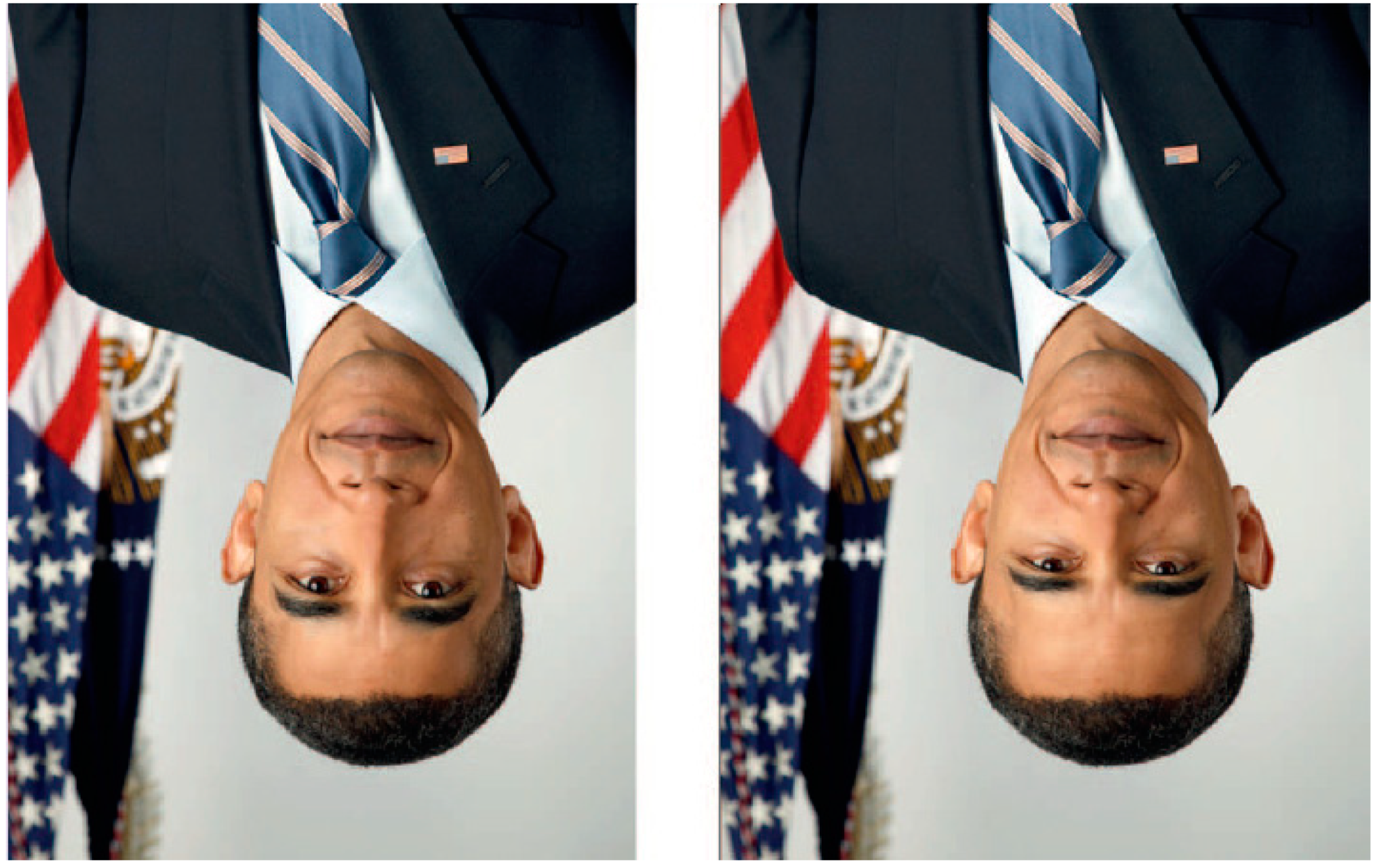
In another experiment (See Figure 1), the configural information in the faces are altered to the point of being grotesque (eyes are placed closer to each other, shorter mouth to nose spatial relation, etc.). When those altered faces were presented in an inverted orientation, the “distinctiveness impressions caused by distorted configural information disappeared” [1,6]. The brain recalls from memory, holistic representation of the face that is free of distortion.

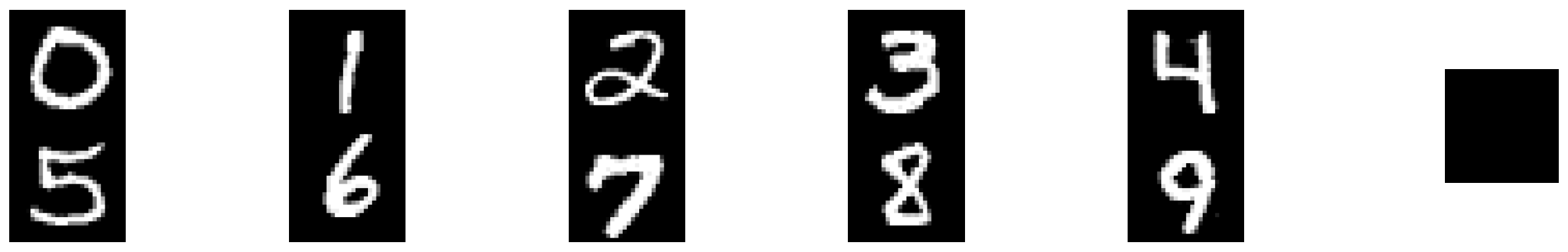
The computational model outlined in Section 2.2.1 is a simplified version of the biological model we just described. To keep it simple, we focus on handwritten digit recognition instead of face recognition. While this recognition task does not have some of the challenges of a face recognition task, such as detection, illumination, occlusion, aging, expression changes, and so on, it does have a few challenges, such as, orientation, in-class variations (Figure 2) to name a few. Thus, a sound engineering model is still necessary to achieve high prediction accuracy. To accurately replicate the biological model, our computational model must decompose the recognition task into two simpler tasks: The first sub-system is specialized in taking as input a digit in any configuration or orientations, and transforms it into a holistic representation with a default orientation learned using supervised learning. The second sub-system uses the holistic representation generated by the first network to perform the recognition. Once we have a model that can take any variation of handwritten digits and transform it into a standard template, classifying the resulting template becomes trivial and can be done with any weak classifier.

The remaining of the paper is organized as follows. Section 2.1, explores related work, Section 2.2 provides a detailed overview of the Variational Autoencoder (VAE) network architecture used to transform the input. In Section 3, we explain the dataset used in the experiment, the training and analysis of the experimental results. In Section 4, we discuss how to interpret the result. We conclude in Section 5.

2.1. Related Work

This section reviews related work in the area of invariant feature extractions, holistic processing and holistic representation of images. The idea of performing recognition using a holistic approach is not new. The oldest holistic model is the Principle Component Analysis (PCA) first proposed by Pearson in 1907 [16]. It a statistical-based approach that creates an average or Eigenface based on the entire training images express in a reduced format or dimension. Recognition is performed by representing the sample input as a linear combination of basis vectors and comparing it against the model. PCA operates holistically without any regard to the “specific feature of the face.” PCA performance suffers under the non-idea condition such as illumination, different background, and affine transformations [17]. Other techniques seek to rectify this shortcoming by trying to integrate feature extraction in a manner that is explicit and, more importantly, invariant to affine transformation. Popular methods are morphological operations (i.e., thresholding, opening, and closing), pre-engineered filters (i.e., Scale-Invariant Feature Transform (SIFT) and Haar-like features), dynamically calculated filters using Hu transforms and learned filters using a Convolutional Neural Network [18].

The authors of [19] present a handwritten digit classifier that extracts features (i.e., contours) using morphological operations, then performs classification by computing the similarity distance of the Fourier coefficients from those features. The recognition rate for 5000 samples, provided by ETRI (Electronic and Telecommunications Research Institute), was 99.04%.

In [20], feature extraction that is invariant was achieved by using filters that have invariant properties as well as by “computing features over concentric areas of decreasing size.” The authors used both normalized central moments and moment invariant algorithms to compute invariant feature extractors as a pre-processing step to object recognition. As many as 12 normalized central moments are needed to calculate filters invariant to scale; however, these filters are not invariant to rotate. The authors also used another 11 independent moments, which are based on Flusser’s set and Hu’s moment invariant theory. These filters are scale and rotational invariant. Once the features were extracted, the classification was done using a modified version of the AdaBoost algorithm. Misclassifications were reported as high as 56.1% and as low as 9.5% [20]. The disadvantage of engineer filters is their inability to generalize.

Another method of extracting features is where the feature extractor learns the appropriate filters. The model trainable feature extractor in [21] was based on the LeNet5 convolutional network architecture. To improve the recognition performance, the authors used affine transformations and elastic distortions to create additional tanning data, in addition to the original 60,000 training data from the Modified National Institute of Standards and Technology (MNIST) dataset [22]. The result of the experiments reported a recognition rate of 99.46%.

The architecture most similar to our model, is the learning model proposed by [23]. The architecture is an encoder-decoder model, which encode the feature using four binary numbers (the code), and a decoder that reconstructs the input based on that code. The objective was to create a model that can learn invariant features in an unsupervised fashion. The authors stated that the invariance comes from max-pooling, a method that was first introduced in the CNN [18] and by learning a feature vector (i.e., the code), using the encoder-decoder architecture, that incorporates both “what” is in the image and “where” it is located. The model achieved an error rate of 0.64% when trained using the full training set of the MNIST dataset.

To develop a computational model that mimics how our brain performs recognition, we use a generative model, follow by a classifier. While a Generative Adversarial Network (GAN) or a vanilla autoencoder would be suitable generators, a variational autoencoder is ideal because it matches the biological model’s ability to learn invariant features. In this paper, we propose an architecture that is based on a variational autoencoder, capable of learning features that are invariant to all the transformations. Instead of reconstructing the original digit image in its original orientation, the model learns to generate a holistic representation of the image at a 0° position. By using a VAE instead of a vanilla autoencoder, the network learns a distribution of encoding to represent each digit; as a result, it generalizes better [23,24].

2.2. The Network Architecture

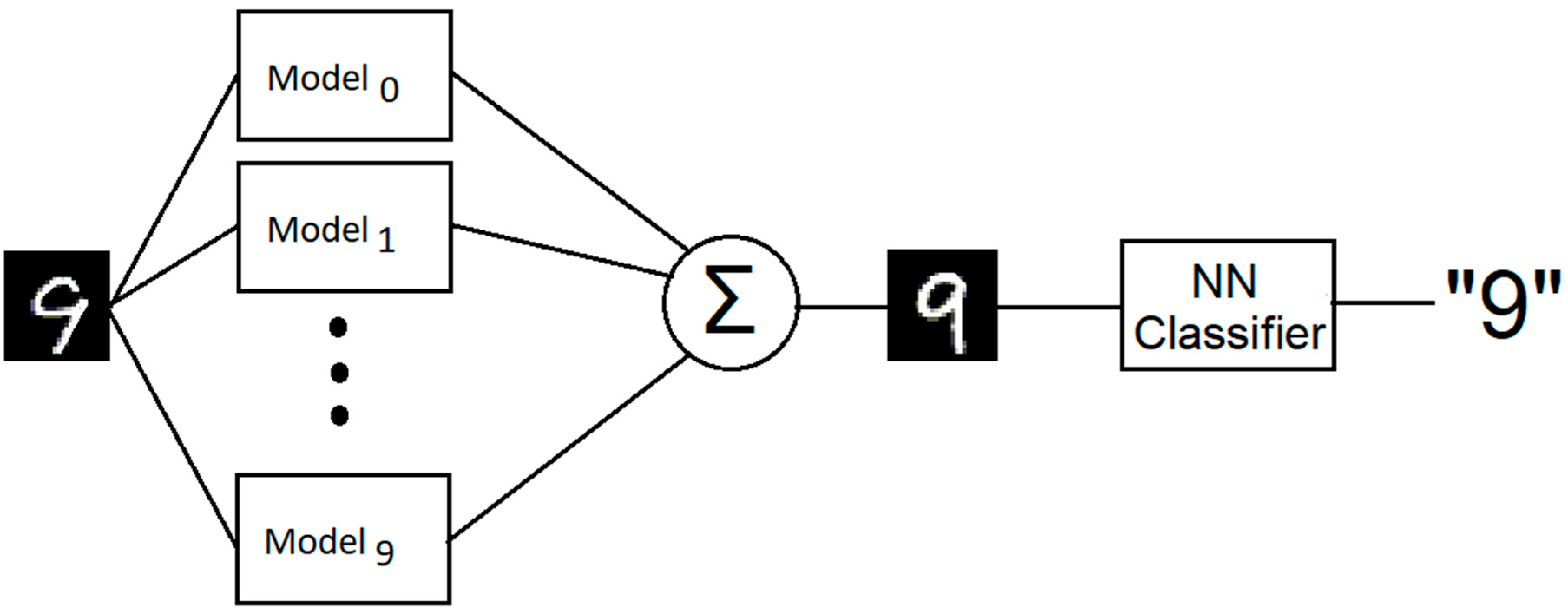
Figure 3 shows a high-level view of our proposed model. The model decomposes the recognition tasks into two sub-tasks: a generator for feature extractions and generation and a Neural Network for classification.

2.2.1. The Generator

The generator is based on the variational autoencoder architecture. The raw input image is 28 × 28 pixels, it is normalized and fed to the first convolution layer, which has 16 feature maps, 7 × 7 kernels and followed by a Rectified Linear Unit (RELU) activation function. Convolutions between the input image and the kernels are performed. Padding is used to retain the size of the input image. This step is followed by a non-linearity and a 2 × 2 max pooling, which produces a 14 × 14 image.

The output of the first convolution layer is fed to the second convolution layer with 32 feature maps, 7 × 7 kernels. Convolutions are performed again with padding so that the size of the input image is retained, followed by an RELU non-linearity and 2 × 2 max pooling. The resulting output is a 7 × 7 image.

The output of the convolutional layers is flattened and fed to a fully connected encoder neural network. The encoder is made of two layers of 512 and 128 neurons, respectively, with a Tanh activation function. The output of the encoder is fed in parallel to two layers made of 7 neurons each, referred to as mean and variance. These layers are used to calculate the compress representation of the input image, also referred to as the probabilistic latent vector Z, or “the code.” This layer is also a vector of size 7, with the goal of representing the extracted features as a probability distribution. It is calculated as follows:

$$\mathrm{Z}= \mu +\epsilon ʘ \mathcal{N}\left(0, 1\right)$$

(1)

where $\mu$ is the mean, $\epsilon$ is the variance, $ʘ$ is an element wise multiplication, and $\mathcal{N}\left(0, 1\right)$ is a zero mean and unit variance gaussian distribution.

The chosen distribution is known to be tractable, and the latent vector Z will be forced to follow that distribution through K-L divergent. Our objective for using variational inference, as outlined in the next section, is strictly to learn the distribution of the latent vector Z, not for classification, visualization or data augmentation. The chosen distribution is held constant throughout testing. For more information on VAE, see [24].

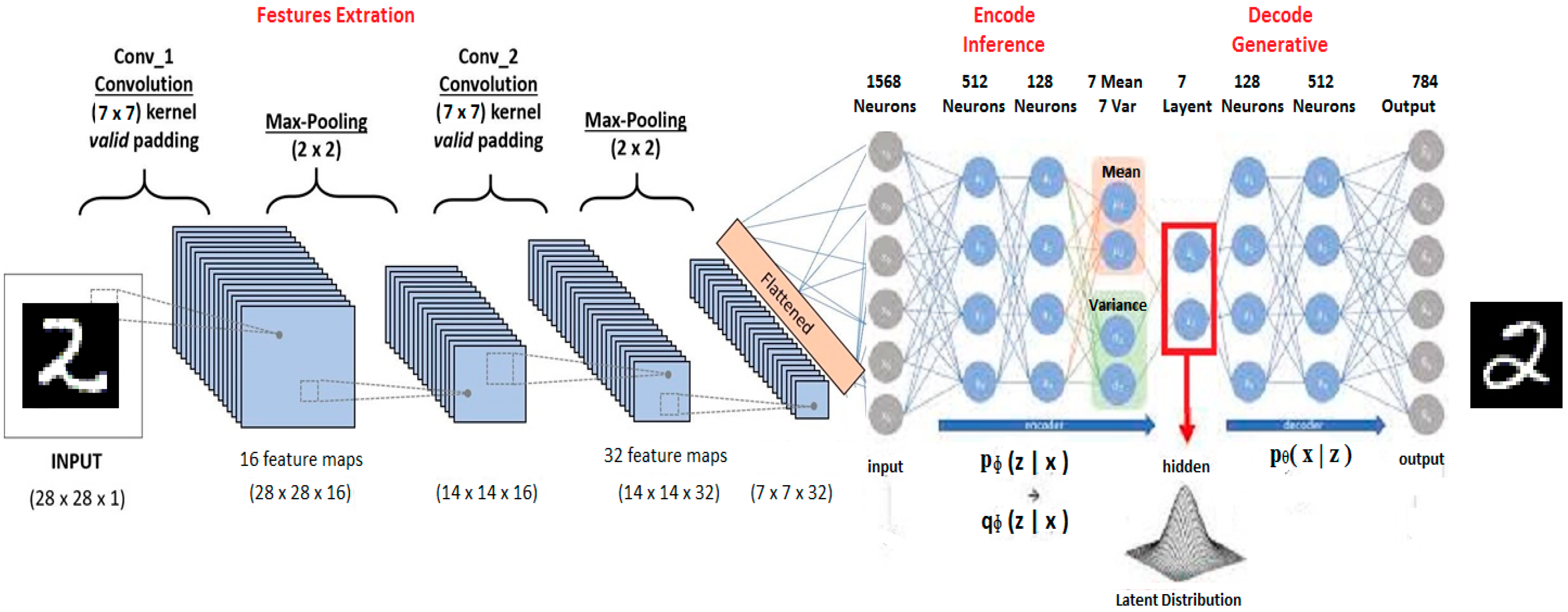
The latent vector is fed to a decoder made of two layers with 128 and 512 neurons, respectively, with an RELU activation function. The final layer is the output layer of 784 neurons with a sigmoid activation function. The generator is shown in Figure 4.

The hyperparameters for the model were chosen through experiments and are determined to be optimal. For instance, we found that using 2 convolution layers with 8 kernels in the first layer and 16 kernels in the second layer was insufficient to produce good results, while using 32 kernels in the first CNN and 64 in the second produced diminishing returns. Experiments with a latent vector of size 2 or 3 impeded the network ability to converge. On the other hand, any latent vector size above 8 was more than needed.

2.2.2. The Classifier

The output vector of each generator is summed and fed to a classifier. The classifier is a neural network with one hidden layer of 256 neurons with a Tanh activation function and an output layer with ten neurons, one for each of digit class. A SoftMax activation is used in the output layer. The Softmax function express the output of the classifier, as a level of confidence that the given input belongs to that class. The output with the highest probability represents the network prediction. The sum probability of all the output is equal to one. The Softmax function is given by:

$${\stackrel{\leftharpoonup }{\mathrm{H}}}_{\mathrm{j}\mathrm{k}}\left(x\right)=\frac{{\mathrm{e}}^{{\mathrm{H}}_{\mathrm{j}\mathrm{k}}\left(x\right)}}{{{\displaystyle \sum }}_{\mathrm{l}=1}^{\mathrm{N}}\left({\mathrm{e}}^{{\mathrm{H}}_{\mathrm{j}\mathrm{l}}\left(x\right)}\right)}$$

(2)

The objective was to use a weak final classifier so that the overall performance of the architecture is attributed solely to the model. The parameters used in the final classifier NN were chosen because they are standard for a weak classifier and the performance of such a network is well established.

2.2.3. Variational Autoencoder

Variational Autoencoder architecture is based on autoencoders. It has an encoder and decoder just like autoencoders; however, VAE encodes each feature using a distribution, which allows the network to generalize better.

So, the goal of the variational autoencoder is to find a distribution P_θ(z|x) of some latent variables, so that new data can be sampled from it.

Using Bayesian statistics, we have:

$$\mathrm{p}\left(\mathrm{z} | \mathrm{x}\right)=\frac{\mathrm{p}\left(\mathrm{x} | \mathrm{z}\right)\mathrm{p}\left(\mathrm{z}\right)}{\mathrm{p}\left(\mathrm{x}\right)}$$

(3)

$$\mathrm{p}\left(\mathrm{x}\right)=\underset{\mathrm{z}}{{\displaystyle \int }}\mathrm{p}\left(\mathrm{x}|\mathrm{z}\right)\mathrm{p}\left(\mathrm{z}\right)\mathrm{dz}$$

(4)

Given that the latent space, z, can be any dimension, we would have to calculate the integral for each dimension. Therefore calculating p(x), the marginal likelihood, is not tractable.

If we cannot compute p(x),then we cannot compute p(z|x).

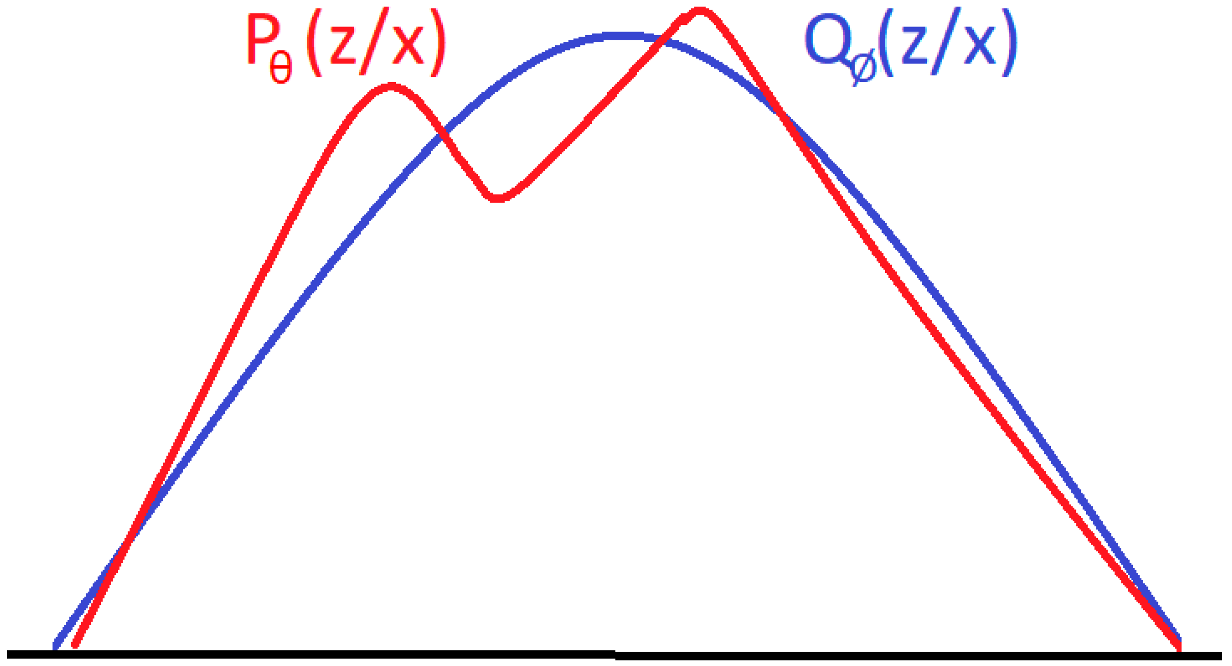
To solve this problem, we use variational inference to approximate this distribution. To find an approximation to the truly intractable p_θ(z|x), we will introduce a known (tractable) distribution q_ϕ(z|x) and force p_θ(z|x) to follow this distribution, without interfering with the generation of the holistic image. We will use a method known as K–L divergent [24]. K–L divergent is a method for measuring similar distributions. The goal is to find ϕ that makes q closest to p_θ (see Figure 5).

The formula for K–L divergent is:

$${\mathrm{D}}_{\mathrm{k}\mathrm{l}}\left[ \mathrm{q}\left(\mathrm{x}\right)\left|\right|\mathrm{p}\left(\mathrm{x}\right)\right]= \sum \mathrm{q}\left(\mathrm{x}\right)\log \left(\frac{\mathrm{q}\left(\mathrm{x}\right)}{\mathrm{p}\left(\mathrm{x}\right)}\right)$$

(5)

If we replaced p(x) and q(x) with conditional probabilities, we got:

$${\mathrm{D}}_{\mathrm{k}\mathrm{l}}\left[{\mathrm{Q}}_{\mathsf{\varphi }}\left(\mathrm{z}|\mathrm{x}\right)\left|\right|{\mathrm{P}}_{\mathsf{\theta }}\left(\mathrm{z}|\mathrm{x}\right)\right]= \sum \mathrm{q}\left(\mathrm{z}|\mathrm{x}\right)\log \left(\frac{\mathrm{q}\left(\mathrm{z}|\mathrm{x}\right)}{\mathrm{p}\left(\mathrm{z}|\mathrm{x}\right)}\right)$$

(6)

The equation is rewritten as an expectation:

$${\mathrm{D}}_{\mathrm{k}\mathrm{l}}\left[{\mathrm{Q}}_{\mathsf{\varphi }}\left(\mathrm{z}|\mathrm{x}\right)\left|\right|{\mathrm{P}}_{\mathsf{\theta }}\left(\mathrm{z}|\mathrm{x}\right)\right]= {\mathrm{E}}_{\mathrm{z}~{\mathrm{Q}}_{\mathsf{\varphi }}(\mathrm{x}|\mathrm{z})}[ \log \left(\frac{{\mathrm{Q}}_{\mathsf{\varphi }}\left(\mathrm{z}|\mathrm{x}\right)}{{\mathrm{P}}_{\mathsf{\theta }}\left(\mathrm{z}|\mathrm{x}\right)}\right) ]$$

(7)

Substituting ${\mathrm{P}}_{\mathsf{\theta }}\left(\mathrm{z}|\mathrm{x}\right)$ with Equation (3) using Bayes’ and log rules, we got:

$$\begin{array}{l}{\mathrm{D}}_{\mathrm{k}\mathrm{l}}[ {\mathrm{Q}}_{\mathsf{\varphi }}(\mathrm{z}|\mathrm{x})\left|\right|{\mathrm{P}}_{\mathsf{\theta }}\left(\mathrm{z}|\mathrm{x}\right)\\ \hspace{1em}\hspace{1em}= \mathrm{l}\mathrm{o}\mathrm{g} \mathrm{p}\left(\mathrm{x}\right) - {\mathrm{E}}_{\mathrm{z}}[\mathrm{l}\mathrm{o}\mathrm{g}({\mathrm{P}}_{\mathsf{\theta }}(\mathrm{x}|\mathrm{z}))\left] + {\mathrm{D}}_{\mathrm{k}\mathrm{l}}\right[{\mathrm{Q}}_{\mathsf{\varphi }}(\mathrm{z}|\mathrm{x})|{|\mathrm{P}}_{\mathsf{\theta }}\left(\mathrm{z}\right)] \end{array}$$

(8)

Since D_kl is always positive, then we can conclude,

$$\mathrm{L}\mathrm{o}\mathrm{g} \mathrm{P}\left(\mathrm{x}\right) >= {\mathrm{E}}_{\mathrm{z}}[\mathrm{l}\mathrm{o}\mathrm{g}({\mathrm{P}}_{\mathsf{\theta }}(\mathrm{x}|\mathrm{z}))\left] – {\mathrm{D}}_{\mathrm{k}\mathrm{l}}\right[{\mathrm{Q}}_{\mathsf{\varphi }}(\mathrm{z}|\mathrm{x})|{|\mathrm{P}}_{\mathsf{\theta }}\left(\mathrm{z}\right)]$$

(9)

Therefore, if we maximize the term on the right-hand side, we are also maximizing the term on the left-hand side. This is why the term on the right-hand side is called estimate likelihood lower bound (ELBO). Likewise, if we minimize D_kl[Q_ϕ(z|x)||P_θ(z)] (because of the minus sign), then we are maximizing E_z[log(P_θ(x|z))] where E is the Expectation of a certain event occurring.

Therefore, the loss function for variational autoencoder is:

$$\mathrm{L}\left(\mathsf{\theta }, \mathsf{\varphi }\right)= -{\mathrm{E}}_{\mathrm{z}~{\mathrm{Q}}_{\mathsf{\varphi }}(\mathrm{x}|\mathrm{z})} [\mathrm{l}\mathrm{o}\mathrm{g}({\mathrm{P}}_{\mathsf{\theta }}(\mathrm{x}|\mathrm{z})] + {\mathrm{D}}_{\mathrm{k}\mathrm{l}} \left({\mathrm{Q}}_{\mathsf{\varphi }}\left(\mathrm{z}|\mathrm{x}\right)\left|\right|{\mathrm{P}}_{\mathsf{\theta }}\left(\mathrm{z}\right)\right)$$

(10)

So, to compute D_kl[Q_ϕ(z|x)||P_θ(z)], we estimate the unknown distribution with the known distribution $\mathcal{N}\left(0, 1\right)$.

Suppose we have two multivariate normal distributions defined as:

$$\mathrm{P}\left(\mathrm{x}\right)= \mathcal{N}\left(\mathrm{x}, {\mu }_1, {\epsilon }_1\right)$$

(11)

$$\mathrm{Q}\left(\mathrm{x}\right)= \mathcal{N}\left(\mathrm{x}, {\mu }_2, {\epsilon }_2\right)$$

(12)

where ${\mu }_1$ and ${\mu }_2$ are means, and ε₁ and ε₂ are the covariance matrix or variance.

The multivariate normal density distribution of dimension k is defined as:

$$\mathcal{N}\left(\mathrm{x}, \mathrm{u}, \epsilon \right)=\frac{1}{\sqrt{{\left(2\mathsf{\pi }\right)}^{\mathrm{k}}|\epsilon |}}{\mathrm{e}}^{-0.5 {\left(\mathrm{x}-\mu \right)}^{\mathrm{T}}{\epsilon }^{-1}\left(\mathrm{x}-\mu \right)}$$

(13)

$$\begin{array}{l}{\mathrm{D}}_{\mathrm{k}\mathrm{l}}(\mathrm{p}\left(\mathrm{x}\right)||\mathrm{q}\left(\mathrm{x}\right)) \\ \hspace{1em}\hspace{1em}\hspace{1em}\hspace{1em}= ½ [ \log \frac{\left|{\epsilon }_2\right|}{\left|{\epsilon }_1\right|} – \mathrm{d} + \mathrm{trace}\left({\epsilon }_2{}^{-1} {\epsilon }_1{}^{-1}\right)\\ \hspace{1em}\hspace{1em}\hspace{1em}\hspace{1em}+ \left({\mu }_2-{ \mu }_1\right) {\epsilon }_2{}^{-1} \left({\mu }_2-{ \mu }_1\right)]\end{array}$$

(14)

If we set one of the distributions to be zero mean and the unit variance as $\mathcal{N}$(0, 1), then:

$${\mathrm{D}}_{\mathrm{k}\mathrm{l}}\left[\mathcal{N}\left(\mu , \epsilon \right) \left|\right| \mathcal{N}\left(0, 1\right)\right]=\frac{1}{2}{\displaystyle \sum }_{\mathrm{j}=1}^{\mathrm{J}}\left(1+\log \left({\epsilon }^2\right)- {\mu }^2- {\epsilon }^2\right)$$

(15)

To solve the term ${\mathrm{E}}_{\mathrm{z}~{\mathrm{Q}}_{\mathsf{\varphi }}(\mathrm{x}|\mathrm{z})} [\mathrm{l}\mathrm{o}\mathrm{g}\left({\mathrm{P}}_{\mathsf{\theta }}\left(\mathrm{x}|\mathrm{z}\right)\right]$ in Equation (10), we use re-parameterization trick.

Re-Parameterization

To minimize a loss function, we take the partial derivative with respect to one of the model parameters and set it to zero. It turns out that it is difficult to take the derivative of this loss function with respect to ϕ, because the expectation is taken over the distribution, which is dependent on ϕ. This is why a re-parameterization trick is required. Re-parameterization involves using a transformation to rewrite the expectation ${\mathrm{E}}_{\mathrm{z}~{\mathrm{Q}}_{\mathsf{\varphi }}(\mathrm{x}|\mathrm{z})}$ in such a way that the distribution is independent of the parameter ϕ. So, an expectation of the form ${\mathrm{E}}_{\mathrm{z}~{\mathrm{Q}}_{\mathsf{\varphi }}(\mathrm{x}|\mathrm{z})} \left[\mathrm{f}\left(\mathrm{z}\right)\right]$ can be re-written as ${\mathrm{E}}_{\mathrm{P}(ꞓ)} \left[\mathrm{f}\left({\mathrm{G}}_{\mathsf{\varphi }}\left(ꞓ, \mathrm{x}\right)\right)\right]$. P(ꞓ) (reads probability of epsilon), is sampled from a gaussian distribution with zero mean and unit variance (i.e., ꞓ~$\mathcal{N}\left(0, 1\right)$). If we set ${\mathrm{G}}_{\mathsf{\varphi }}\left(ꞓ, \mathrm{x}\right)$ to be equal to a standard linear transformation ${\mu }_{\mathsf{\varphi }}\left(\mathrm{x}\right)+ ꞓ ʘ \sqrt{{\epsilon }_{\mathsf{\varphi }}}$, then we can obtain a gaussian function of arbitrary mean and variance, $\mathcal{N}\left(\mu \left(\mathrm{x}\right), \epsilon \left(\mathrm{x}\right)\right)$, from the gaussian $\mathcal{N}\left(0, 1\right)$. This means we are transforming $\mathcal{N}\left(0, 1\right)$ to $\mathcal{N}\left(\mu \left(\mathrm{x}\right), \epsilon \left(\mathrm{x}\right)\right)$. Therefore, instead of sampling z from ${\mathrm{Q}}_{\mathsf{\varphi }}\left(\mathrm{x}|\mathrm{z}\right),$ we instead sampled it from ${\mathrm{G}}_{\mathsf{\varphi }}\left(ꞓ, \mathrm{x}\right)$.

$${\mathrm{E}}_{\mathrm{z}~{\mathrm{Q}}_{\mathsf{\varphi }}(\mathrm{x}|\mathrm{z})}= {\mathrm{E}}_{\mathrm{P}(\epsilon )} \left[\mathrm{f}\left({\mathrm{G}}_{\mathsf{\varphi }}\left(\epsilon , \mathrm{x}\right)\right)\right]$$

(16)

$$\begin{array}{c}{\mathrm{E}}_{\mathrm{z}~{\mathrm{Q}}_{\mathsf{\varphi }}(\mathrm{x}|\mathrm{z})} [\mathrm{l}\mathrm{o}\mathrm{g}\left({\mathrm{P}}_{\mathsf{\theta }}\left(\mathrm{x}|\mathrm{z}\right)\right]\equiv {\mathrm{E}}_{\mathrm{Z} ~ \mathrm{P}(\epsilon )} \left[{\log \mathrm{P}}_{\mathsf{\theta }}(\mathrm{x} |{\mathrm{z}}^{\mathrm{l}})\right]\equiv \\ \frac{1}{\mathrm{L}}{{\displaystyle \sum }}_{\mathrm{l}=1}^{\mathrm{L}}{\log \mathrm{P}}_{\mathsf{\theta }}(\mathrm{x} |{\mathrm{z}}^{\mathrm{l}})\end{array}$$

(17)

where ${\mathrm{z}}^{\mathrm{l}}$ comes from the transformation ${\mu }_{\mathsf{\varphi }}\left(\mathrm{x}\right)+ ꞓ\ast \sqrt{{\epsilon }_{\mathsf{\varphi }}}$ and $ꞓ$ is sampled from $\mathcal{N}\left(0, 1\right)$. This allows us to obtain the Monte-Carlo estimate of the expectation in a form that is differentiable. For more information on re-parameterization, we refer the reader to [24].

The K-L Divergent Loss Function

Plugging (15) and (17) into (10), give the complete VAE loss function:

$$\begin{array}{l}\mathrm{L}\left(\mathsf{\theta }, \mathsf{\varphi }\right)= -\frac{1}{\mathrm{L}}{\displaystyle \sum _{\mathrm{l}=1}^{\mathrm{L}}}{\mathrm{logP}}_{\mathsf{\theta }}(\mathrm{x} |{\mathrm{z}}^{\mathrm{l}}) \\ \hspace{1em}\hspace{1em}\hspace{1em}\hspace{1em}+ \frac{1}{2}{\displaystyle \sum _{\mathrm{j}=1}^{\mathrm{J}}}\left(1+\log \left({\epsilon }^2\right)- {\mu }^2- {\epsilon }^2\right)\end{array}$$

(18)

The first term is the data fidelity loss, and the second term is the K–L divergent [24].

The Generator Loss-Function

As stated earlier, there are ten identical generators, and each generator network is trained to generate a different holistic digit. To prevent the network from learning the identity function, each network is trained with both similar digit and dissimilar digits. In every batch, half of the training data are composed of the digit the network is learning to generate, and we will refer to them as a similar digit. The other half of the training data is randomly chosen from the full training dataset (excluding similar digit), we will refer to them as dissimilar digits. As a result, we replace the data fidelity term in Equation (11), with the contrastive loss function [25]. With the usage of a conditional parameter $\mathrm{Y},$ the contrastive loss function accommodates two optimization paths, one when the ground truth is similar to the input and another when they are dissimilar. For more information on contrastive loss, we refer the reader to [25].

Let x and $\stackrel{᷈}{\mathrm{x}}$ represent the ground truth (see Figure 6) and the generated images, respectively.

Let Y be a binary label assigned to this pair, such that Y = 1 when x and x᷈ are expected to be similar, and Y = 0 otherwise.

The absolute distance (or L1Norm) is given by:

$${\mathrm{D}}_{\mathsf{\theta }}= {\sum }_{\mathrm{l}=1}^{\mathrm{L}}\left|\mathrm{x}-\stackrel{᷈}{\mathrm{x}}\right|$$

(19)

$$\mathrm{L}\left(\mathsf{\theta }\right)= \frac{1}{2}\mathrm{Y} {\mathrm{D}}_{\mathsf{\theta }}{}^2+\frac{1}{2}\left(1-\mathrm{Y}\right) {\left(\mathrm{M}\mathrm{a}\mathrm{x}\left[0, \mathrm{m}-{\mathrm{D}}_{\mathsf{\theta }}\right]\right)}^2$$

(20)

The Contrastive loss as defined in [25] is:

The margin m, defines the radius around which dissimilar digits contribute to the loss function. When $\mathrm{Y}=0$ and m < D_θ, then no loss is incurred. Since the objective is for dissimilar digits to contribute equally to the learning process, m is set to a number greater than one (i.e., m = 5).

Replacing the reconstruction likelihood $\frac{1}{\mathrm{L}}{{\displaystyle \sum }}_{\mathrm{l}=1}^{\mathrm{L}}{\mathrm{logP}}_{\mathsf{\theta }}(\mathrm{x} |{\mathrm{z}}^{\mathrm{l}})$ in Equation (18) yields:

$$\mathrm{L} \left(\mathsf{\theta }, \mathsf{\varphi }\right)= -\frac{1}{2}\mathrm{Y} {\mathrm{D}}_{\mathsf{\theta }}{}^2+\frac{1}{2}\left(1-\mathrm{Y}\right) {\left(\mathrm{M}\mathrm{a}\mathrm{x}\left[0, \mathrm{m}-{\mathrm{D}}_{\mathsf{\theta }}\right]\right)}^2+ \frac{1}{2}{\displaystyle \sum }_{\mathrm{j}=1}^{\mathrm{J}}\left(1+\log \left({\epsilon }^2\right)- {\mu }^2- {\epsilon }^2\right)$$

(21)

3. Dataset and Training Strategy

The results of the experiments using the MNIST database [22] are outlined in this section. The database is a well-known benchmark with 60,000 training images and 10,000 test images. The images are 28 × 28 pixels gray-level bitmaps with digits centered in a frame in white with a black background. As a result, digit detection is not necessary, since the digit is the only object in the image. The entire 60,000 images are used as training inputs to train the generator. The ground truth images that are used as labels are carefully chosen from the training set to be as differentiable as possible (Figure 6). They are the holistic representation the generator is expected to reconstruct. Another set of 50 images, five from each class, were randomly chosen from the training set, and are used as a validation set.

To reduce the resource necessary to train the network, the model uses a separate network for each digit without sharing model parameters. Each generator network is trained separately for 200 epochs using the full 60,000 training set. Due to the probabilistic nature of the network, some digits required more training than others. Starting at epoch 100, the model’s progress is monitored using the validation set, and a snapshot of the model is saved for all 100% success rate. Success in this context is defined as the model’s ability to reconstruct the digit being trained for or produce a blank image for all other digits (see Figure 3). Once training is over, a stable checkpoint is chosen for further integrated training. A model is deemed stable if, during training, it has at least 3 consecutives success using the validation set.

The classifier Neural Network is trained separately for 50 epochs on the full training dataset.

4. Results and Discussion

We calculate the success rate S (or accuracy) as the total number of digits correctly predicted by the network or true positive (TP), divided by the number of total numbers of test data (TD). Therefore:

$$S=\frac{TP+TN }{TD}$$

(22)

Consequently, the error rate ER is given by (1—S) or:

$$ER=\frac{FP+FN}{TD}$$

(23)

The integrated architecture achieves a 99.05% accuracy in the recognition task, which is near state of the art, when compared to the best-published results on this dataset [26] and done so without augmenting the dataset or pre-processing. Since the integrated architecture summed the output of all the individual models, any false positive error resulted in an overlap representation of two or more holistic images. As a result, the composite image is un-recognizable by the final classifier (see Figure 3). This adversely affects the accuracy of the integrated architecture. To demonstrate the model’s superior ability to recognize and reconstruct the digit for which it is trained for, ten more experiments were conducted, one for each digit. The results show an overall true positive accuracy of 99.5%.

Table 1. Individual model experimental results.

	Model 0	Model 1	Model 2	Model 3	Model 4	Model 5	Model 6	Model 7	Model 8	Model 9	Overall
Similar Digits	980	1135	1032	1010	982	892	958	1028	974	1009	10,000
Dissimilar Digits	9020	8865	8968	8990	9018	9108	9042	8972	9026	8991	90,000
False Negative	0	0	0	7	9	6	7	6	5	10	0.50%
False Positive	6	8	16	8	7	12	10	10	13	13	0.11%

shows the raw data of the experiments. For instance, the test conducted on the model that was trained for digit seven yields an accuracy of 99.84%. As shown in Table 1, the test set contains a total of 1028 images for digit seven (similar digits or expected true positive) and 8972 images for the other digits (dissimilar digits or expected true negative), 10,000 test images all together. The result shows 6 cases when the model erroneously generated a blank image for a valid input image of the digit seven (false negative) and 10 cases when it generated the holistic representation of digit seven, when in fact the input image was not the digit seven (false positive). Given this information and Equation (22), the success rate for the model trained for digit seven is computed as follows:

$$\mathrm{S} = \frac{1018 + 8966 }{10000} = 99.84\%.$$

The lowest accuracy recorded was 99.77% for the model trained for digit nine and the best accuracy was 99.94% for the model trained for digit zero (or error rates from 0.23% to 0.06%).

The most extensive and recent survey of recognition models using the MNIST and the Extended MNIST (EMNIST) dataset was published in the paper, “A Survey of Handwritten Character Recognition with MNIST and EMNIST”. Among them are 44 models that achieve accuracy similar to ours, that is accuracy greater than 99% (or error < 1%) using the MNIST dataset without data augmentation or preprocessing. The error rates reported ranged from 0.95% to 0.24% [26]. Among them, 37 use CNN for feature extraction followed by an algorithm and or a neural network to perform the classification. The fact there are no simpler model (i.e., less than two convolution layers and fewer kernels) with results similar to ours confirms our hypothesis.

The handwritten digit recognition was chosen to demonstrate the model because it is a much simpler problem than face recognition. The logical next step is to apply it to face recognition.

5. Conclusions

This paper proposed a classifier for handwriting digit recognition based on a model that first transforms the input to a holistic or average representation and then performs classification based on that template. The experimental results using the MNIST dataset show that such a strategy allows the network to learn features that are invariant to all the transformations included in the dataset. The integrated architecture achieved near state-of-the-art recognition, and the model demonstrated a superior ability individually to recognize and reconstruct digits, when compared to the best-published results on this database, and did so without pre-processing or augmenting the dataset.