1. Introduction
The class of nonlinear beta regression models was proposed by [
1] and extended to situations in which the data include zeros and/or ones by [
2,
3]. Shortly thereafter, [
4] developed for the class of nonlinear beta regression model residuals and measures of local influence. Local influence proposed by [
5] is a decisive scheme to select the model that fit well a dataset, takes into account that the estimation process is robust in influential cases. Indeed, the final conclusion about model selection should consider the analysis of influence. The model selection is a crucial step in data analysis, since all inference performance is based on the selected model. [
6] evaluated the behavior of different model selection criteria in a beta regression model, such as the Akaike Information Criterion (AIC) [
7], Schwarz Bayesian Criterion (SBC) [
8] and various approaches based on pseudo-
.
However, it is common for models selected by the usual selection criteria to present poorly fitted or influential observations. Indeed, the best models selected by the usual criteria do not always present residual plots that validate the goodness-of-fit. Also, current fitting procedures for beta regression are infeasible for high-dimensional data setups and require variable selection based on (potentially problematic) information criteria. Furthermore, the usual selection criteria do not offer any insight about the quality of the predictive values. In this context, [
9] proposed the PRESS (Predictive Residual Sum of Squares) statistic, which can be used as a measure of the predictive power of a model. [
10] proposed a coefficient of prediction based on PRESS, namely
that is similar to the
approach. The
statistic can be used to select models from a predictive perspective [
11]. Moreover, the PRESS statistic presents a close relationship with the Cook distance [
12] and local influence measures [
5], as we shall present here. Hence, the
statistic is a selection criterion that takes into account the impact of the observations poorly fitted by the model, observations with atypical residuals, and cases that exert a disproportional effect on the model estimation process, even affect the inference conclusions, influential cases.
Our main goal is to introduce a PRESS-like machine learning tool and its associated
statistic, as a coefficient of prediction for the class of nonlinear beta regression models. The
statistic is used as a selection criterion for beta regression. We carried out Monte Carlo simulations to evaluate the behavior of the
measure, as well as the behavior of two usual
-like criterion, namely: the
[
6] and
[
13]. We considered a variety of simulation scenarios, as different ranges for the response mean, several sample sizes and values to the precision parameter, five link functions and different model misspecifications. Finally, we present and discuss two applications to real data.
The simulation and application data set results showed that small values of the new criterion are an indication that the robustness of the maximum likelihood estimation procedure of the model in the presence of influential points is worthy of further investigation. This information could not be accessed by usual selection criteria. However, the issue about variability is still better accessed by -like criteria. Thus, the best machine learning strategy is to use the three criteria discussed here to choose the best model, once each one holds on different information.
2. Criterion
Consider the linear model
as the supervised learning procedure, where
Y is a vector
of the responses,
X is a known matrix of covariates (measured features) of dimension
of full rank,
is the parameter vector of dimension
and
is a vector
of errors. We have the least-squares estimators:
, the residual
and the predicted value
where
and
. Notice that we found these quantities in one shot, without doing any sort of iterative optimization. Let
be the least-squares estimate of
without the
tth observation and
be the predicted value of the case deleted, such that
is the prediction error. Thus, for multiple regression, the classic Predictive Residual Sum of Squares statistic named here as PRESS
is given by
where
is the ordinary residual obtained by regressing
y on
X and
is the t
diagonal element of the projection matrix
of this regression.
Now, let
be independent random variables, such that each
, for
, is beta distributed denoted by
, i.e., each
has density function given by
where
and
. Here,
and
, where
. Ref. [
1] proposed the class of nonlinear beta regression models in which the mean of
and the precision parameter can be written as
where
and
are, respectively,
and
vectors of unknown parameters (
;
),
and
are the nonlinear predictors,
and
are vectors of covariates (i.e., vectors of known variables),
,
,
and
. Both
and
are strictly monotonic and twice differentiable link functions. Furthermore,
,
, are differentiable and continuous functions, such that the matrices
and
have full rank (their ranks are equal to
k and
q, respectively). The model’s parameters can be estimated by maximum likelihood (ML). In the
Appendix, we present the log-likelihood function, the score vector and Fisher’s information matrix for the nonlinear beta regression model. Model (
2)–(
3) embodies the beta regression linear model with varying dispersion when the predictors are linear functions of the parameters. In this case,
and
If, in addition, the predictor for
is linear and
is constant through the observations, we arrive at the beta regression model defined [
13].
The beta regression likelihood is inherently nonlinear and there are no closed form expressions for the ML estimators, and their computations should be performed numerically using a nonlinear optimization algorithm for machine learning, e.g., some form of iterative Newton’s method (Newton–Raphson, Fisher’s scoring, BHHH, etc.). To propose a PRESS-like statistic for beta regression, we shall explore the relationship between the Fisher iterative ML scheme and a weighted least square regression. This regression considers pseudo variables as proposed [
14] to build a Cook-like distance that have been used in several classes of regression models. Fisher’s scoring iterative scheme used for estimating
, both to linear and nonlinear regression model, can be written as
where
are the iterations which are carried out until convergence. The convergence happens when the difference
is less than a small, previously specified constant.
From Appendix’s expressions (
A1), (
A2) and from (
4), it follows that the
mth scoring iteration for
, in a class of nonlinear regression model is defined as
where the
tth elements of the vectors
and
are
,
,
,
given in
Appendix, expression (
A3). Furthermore,
,
W,
,
T and
are evaluated at
.
Ref. [
14] suggests that we rewrite the iterative process in (
5) by defining the following vector
such that the equation in (
5) becomes
Upon convergence, we may write the ML estimator of
as
Here,
,
,
and
are the matrices
W,
,
T and
, respectively, evaluated at the ML estimators of
and
. We note that
in (
8) can be viewed as the least-squares estimator of
obtained by regressing the pseudo observation vector
Since we had the expression of
in (
8), several quantities related to the pseudo regression in (
9) may be obtained, as the ordinary residual, the projection matrix, the
and the prediction error. Following [
14] we have that
in which
is the
tth row of the
matrix,
and
, are respectively, the
tth diagonal element of the projection matrix
and the
tth ordinary residual of the pseudo regression in (
8) given by
where
the
tth element of the vector
and
are given in (
8) and (
A3–
Appendix), respectively. We note that
,
and
in (
11) is the
standardized weighted residual 1 [
15]. In what follows we able to define
and the prediction error
Plugging (
10) quantity in (
12) we then obtain that
is
Finally, for the nonlinear beta regression models, the PRESS-like statistic becomes as
It is noteworthy that based on (
11) the expression in (
13) may be written as
in which
It is important to emphasize that
in the PRESS expression given in (
14) is the
standardized weighted residual 2 proposed by [
15] which outperforming the others beta regression residuals in their numerical evaluation. In special, outperforming the ordinary residual
. The weighted residuals are constructed using the difference between the logit of the responses and their fitted means, the main qualities of beta distribution. The same holds to the proposal for the PRESS-like statistic to the class of beta regression.
Indeed, the PRESS also has relationships with influence measures [
16]. Ref. [
12] use a version of the likelihood displacement [
17] to build the Cook’s distance that measures the impact of a given observation on the parameter estimates of the mean sub-model by removing it from the data. Based on approximations for the likelihood displacement, the Cook-like distances have been proposed for several classes of regression models. Focus on beta regression models [
18] obtain an approximation for the version of likelihood displacement to build the Cook’s distance given by
plugging (
16) measure in (
13) we thus obtain that
in which
is the Cook-like distance to the class of beta regression. Furthermore, Ref. [
19] shown that
in which
is the total local influence of observation
t, defined in (
A4). Thus,
, which clarify the relationship of this statistic with the local influence measures. Ref. [
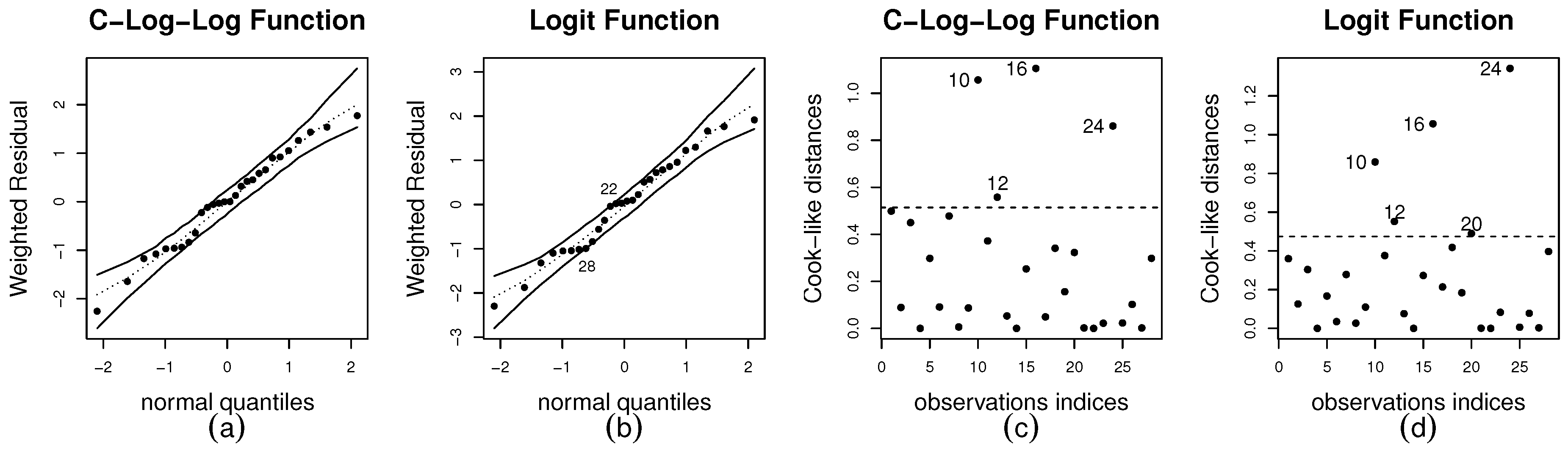
19] also suggest that observations such that
can be taken to be individually influential. We shall take the same threshold pattern to highlight influential observations on the index plots of Cook-like distances. When the predictors in (
3) are linear functions of the parameters, i.e.,
and
the expression in (
17) also represents the PRESS-like statistic for the class of the linear beta regression models with
unknown regression parameters.
Considering the same approach to build the determination coefficient
in linear models, Ref. [
10] define a prediction measure based on the PRESS
statistic in (
1) as
, where
, with
being the arithmetic mean for
values of
.
Based on this idea, for beta regression models we must use the pseudo regression procedure defined in (
9) to build the
-like coefficient as
where
, with
being the arithmetic average for
values of the vector
by excluding the
tth observation. It can be shown that
, wherein
p is the number of model parameters and
is the Total Sum of Squares for the full data. For the class of nonlinear beta regression models,
, where
is the arithmetic average of the
and
. Please note that
given in (
18) is not a positive quantity. Indeed, the
is a positive quantity, thus the
take values in
. The closer to one, the better is the predictive power of the model.
To compare the behaviors of the
defined in (
18) and
-like criteria we consider at the outset two versions of pseudo-
based on the likelihood ratio. The first one was proposed by [
20] as
, where
is the ML achievable (saturated model) and
is the likelihood achieved by the model under investigation. The second version is a proposal of [
6] that takes into account the inclusion of covariates both in the mean and in the precision sub-models, is given by:
where
and
. Based on simulation presented by the authors we chose
and
. We also consider the
, which is defined as the square of the sample coefficient of correlation between
and
[
13], and its penalized version based on [
6] given by
where
and
are, respectively, the number of covariates of the mean and dispersion sub-models. By analogy, we define the penalized version of
given by
3. Simulation Study
The Monte Carlo experiments present in this section were carried out using both fixed and varying dispersion beta regressions as data generating processes, as well as linear and nonlinear models. All simulations were carried out using the
Ox matrix programming language [
21]. The number of Monte Carlo replications is 10,000. Our goal is simultaneously to assess the performance of the
,
and
criteria, and, additionally, which values, on average, these statistics could assume under different data settings and features of the regression model. To that end, at the outset, we present the average values of the statistics as the arithmetic mean of the Monte Carlo replicas. Also, we provide information about the distributions of the statistics by a boxplot analysis.
Since the upper limits of all statistics are equal to one, a performance evaluation criterion for these measures is that their values go to one if the model is correctly specified and far from one otherwise. The mean values of the statistics are especially useful when the scenarios considered in the simulations occur in the real data analysis.
3.1. Linear Setting: Fixed Dispersion, Omitted Covariates and Link Functions
Table 1 shows the mean values of the statistics obtained by simulation of the constant dispersion beta regression model that involves a systematic component for the mean given by
that is based on logit link function. The covariate values were independently obtained as random draws of the following distributions:
,
and were kept fixed throughout the experiment. The precisions, the sample sizes and the range of mean response are, respectively,
,
,
,
and
. Under the model specification given in (
19) we investigate the behavior of the statistics by omitting covariates. In this case, we considered the Scenarios 1, 2, and 3, in which are omitted three, two, and one covariate, respectively. In a fourth scenario, the estimated model is correctly specified.
The results in
Table 1 show that the mean values of all statistics increase as important covariates are included in the model and the value of
increases. On the other hand, as the size of the sample increases, the model misspecification is evidenced by lower values of the statistics (Scenarios 1, 2, and 3). It shall be noted that the mean values for all statistics are considerably larger when
. Additionally, their values approach one when the estimated model is closest to the true model. For instance, in Scenario 4 for
,
the values of
and
are, respectively,
and
.
The behavior of the statistics for finite sample size changes substantially when . It is noteworthy the reduction of its mean values, in special to the criterion when revealing the difficulty in fitting the model in this range of . Even under true specification (Scenario 4) the criterion identifies unmistakably some problem in the model-fitting when . For instance, when and , we have and . The same feature occurs when
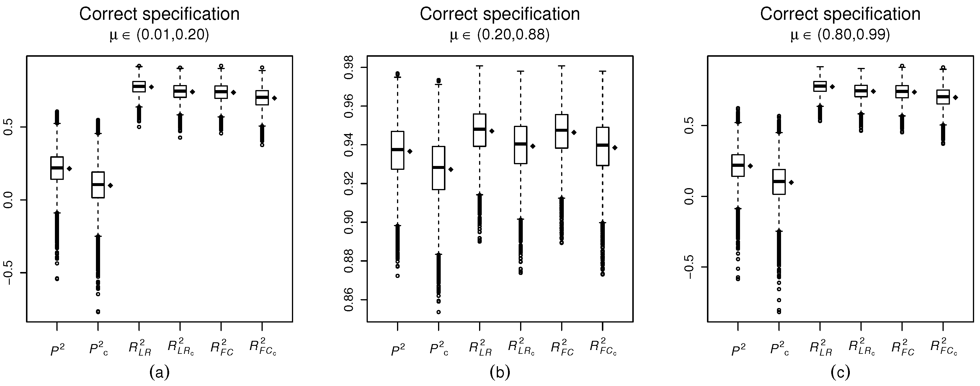
In what follows, we shall investigate the empirical distributions of the statistics:
,
,
,
,
and
under the correctly specified modeling (scenario 4) in
Table 1, for
and
. These results are shown using boxplots of 10,000 values of the statistics obtained from the Monte Carlo simulations (
Figure 1). The mean value of the statistic replications is represented by a dot on the side of each boxplot. In panels (a), (b) and (c) we present the boxplots for
,
scattered on the standard unit interval and for
, respectively.
Figure 1 shows that the means and medians of all statistics are close, thus the mean values of the statistics adequately represent their behavior in these scenarios. We also notice that both
and
criteria are so small, for models correctly specified when
is close to the boundaries of the standard unit interval (
Figure 1). However, it is noteworthy how the
values are substantially smaller than the
-like criterion values.
When the mean response is concentrated on the boundaries of the standard unit interval, even when the model is correctly specified, the statistic of prediction assumes negative values, panel (a) and panel (c). Based on panel (b) (), it can be seen that when the response mean response is scattered on the standard unit interval, the behavior of the prediction statistic is very different, with values much more concentrated nearby one. The same behavior occurs for the goodness-of-fit measures. and .
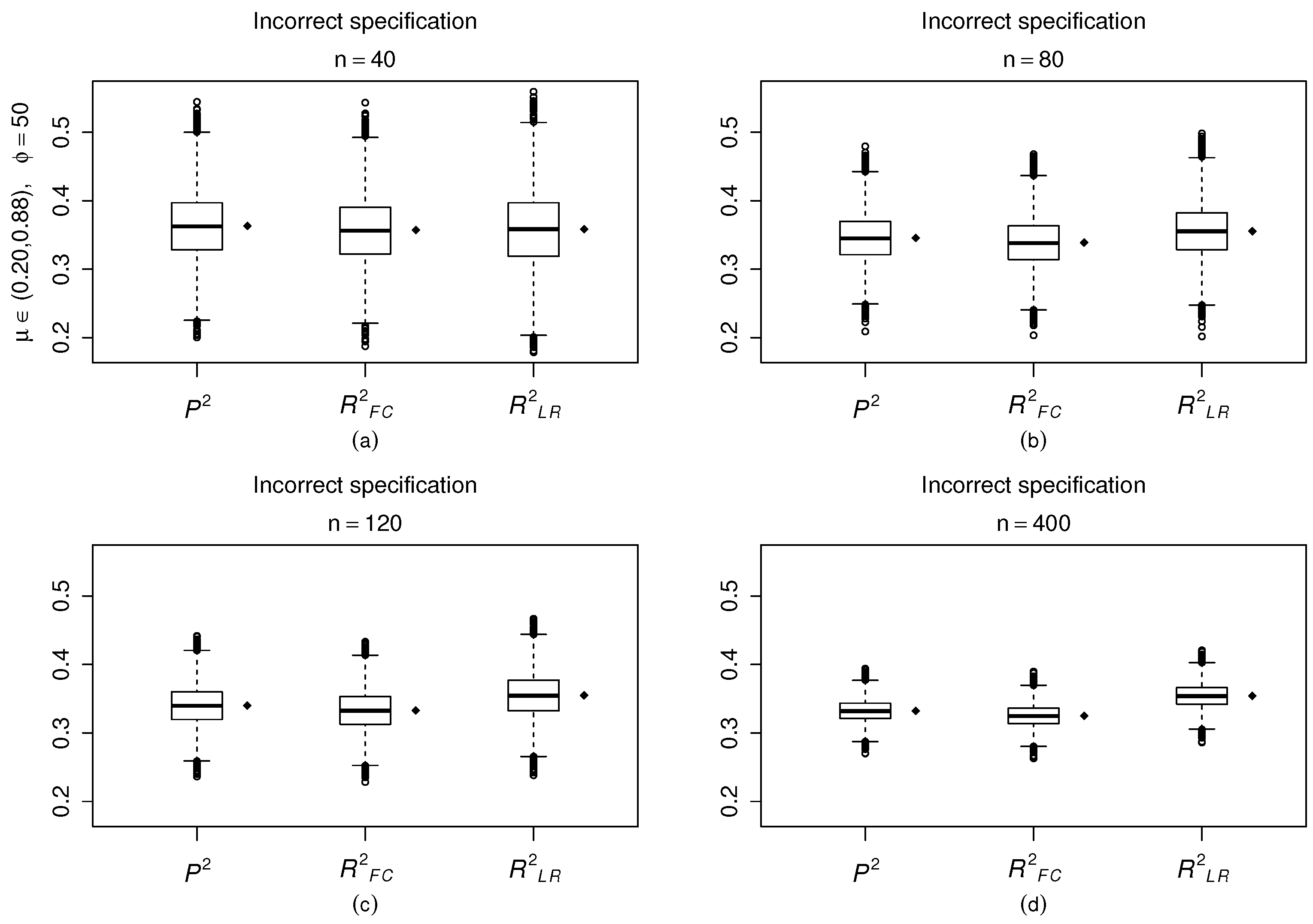
In
Figure 2 we consider a misspecification problem (three omitted covariates). For illustration, we consider only
and
,
. We notice that when three covariates are omitted, with the increasing of sample size, the replication values of the statistics tend to concentrate at small values, as expected due to the misspecification problem.
We notice that typically the mean and the median of the 10,000 values of the statistic is closed, confirming the usefulness of the mean values to describe these measures. When (panel d), the values of all statistics tend to concentrate around a value far from 1, i.e., around and . It behaves noteworthy as the prediction and determination coefficients behave equally in this scenario ().
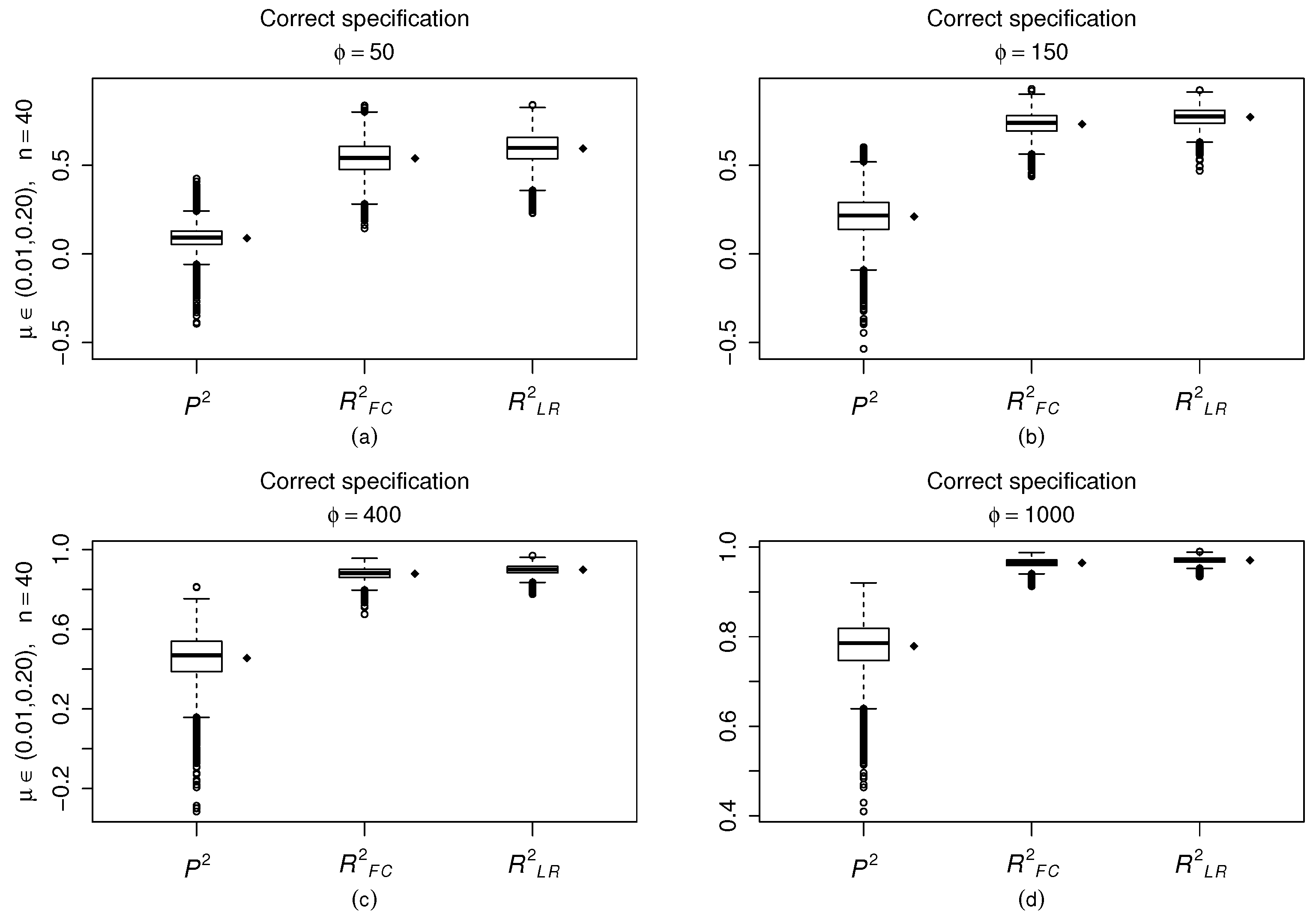
In
Figure 3 we consider
and the model is estimated correctly,
and
. We notice that the values of the
-like statistics become more concentrated and closer to one as the value of
increases. Nonetheless, the behavior of
statistics is quite different. Even when
this measure displays negative values (panel(c)). These observations that present
negative values are cases, poorly fitted by the model and potential influential cases. It is noteworthy that cases poorly fitted by the model can befall in despite of that
(
Figure 3d). The statistics present the same feature when
.
To summarize, at the outset, we shall consider the response mean around . When the model is correctly specified, the have their values close to one, especially when the model precision or sample size increases. When the proposed model omits important covariates, the values tend to depart considerably of one and stay below . The measure and present similar behavior. On the other hand, when the mean of the response is concentrated near zero or one, the values differ considerably from one, taking negative values even when the model is correctly specified, revealing as it is difficult make prediction close to the boundaries of the unit interval.
Indeed, scenarios in which the model present large dispersion and a substantial concentration of values on one of the boundaries of the standard unit interval tend to present influential observations. In these situations, Ref. [
22] argue that for the beta regression models the ML parameter estimation based on the BFGS nonlinear optimization algorithm proved to be typically not robust in influential cases. The
criterion is based on the PRESS-like statistic which presents a relationship both with residuals and influence measures. In this sense, this new criterion that we proposed for the beta regression models outperforms the
and
in identifying problems on fit the model when
or
and the precision is not so large. However, this fact does not disable the use of
-like statistics. The
criterion can be viewed as a measure of model bias whereas the
is a quantifier of the model variance. What we emphasize is that we must also consider the
criterion to select the model that best fit a dataset. In the applications we shall present results that show as the
and
criteria contain different and important information about the model-fitting.
Another important question is the link function to the mean sub-model. All simulations, we carried out until now were based on logit link function. In what follows, we present Monte Carlo simulation results in which we consider other link functions, namely: probit, complementary log–log, log–log, and Cauchy, respectively defined as , , and . It is important to emphasize that the same link function is used both to generate the response observations and to fit the model. Our goal is to evaluate the performance of each link function on different ranges of mean and dispersion response, in special we aim to identifying if the link function is related to the problems in fitting the beta regression model when the response is close of the boundaries of the standard unit interval. Thus, we must fit the model correctly.
The results presented in
Table 2 showed that when the response mean is close to one, the use of complementary log–log function leads to models with better predictive power as well as better goodness-of-fit. On the other hand, if the mean is close to zero the best results are provided by the log–log link function. When the mean is scattered on the standard unit interval both the probit and logit functions perform well. The Cauchy model performance well only when
. Thereby, we can deduce that the link function is related with the small values the
criteria when
and
displayed in
Table 1, since all scenarios were fitted by the logit model. Thus, the appropriate link function can improve the robustness of the ML estimation procedure of the beta models in the presence of influential points. It is noteworthy that these conclusions are supported on the
criterion.
3.2. Linear Setting: Varying Dispersion
In this section, we shall report simulation results to beta regression models with varying dispersion. All results were obtained using 10,000 Monte Carlo replications. Under model misspecification, the true data generating process considers varying dispersion, but a fixed dispersion beta regression is estimated. We also used different covariates in the mean and precision sub-models. The sample sizes are . We generated 40 values for each covariate and replicated them, once, twice, and three times, respectively, to get covariate values for and . Using this procedure, the intensity degree of nonconstant dispersion remains constant as the sample size changes. The numerical results were obtained using the following beta regression model: , , and under different choices of parameters (Scenarios): Scenario 5: , , and Scenario 6: , , , and . Finally, Scenarios 7 and 8 (Full models): , , , , and . Please note that Scenarios 7 and 8 present the same generation data process. However, in Scenario 7 the dispersion is estimated as a constant (misspecification) and in Scenario 8 the dispersion is correctly modeled.
In
Table 3, we present the mean values for 10,000 statistic replications. In this table, we report the results only for
. Next, we presented boxplots for the 10,000 statistic replications to other sample sizes. We are considering
close to
. We notice based on
Table 3 that under model misspecification the statistics display smaller values in comparison with Scenario 8 (correct specification), in which as greater is
greater are the values of the statistics, as expected. When the dispersion is postulated as fixed, as the intensity degree of nonconstant dispersion increases, the mean values of the statistics decreases, which correctly points out for the model misspecification. It is noteworthy that under correct model specification the values of three statistics are so different. In special the
values are greater than the values of
-like criteria. Furthermore, the values of the
are considerably smaller than the values of the
, in special when
increases. For example, taking
,
we have
and
(
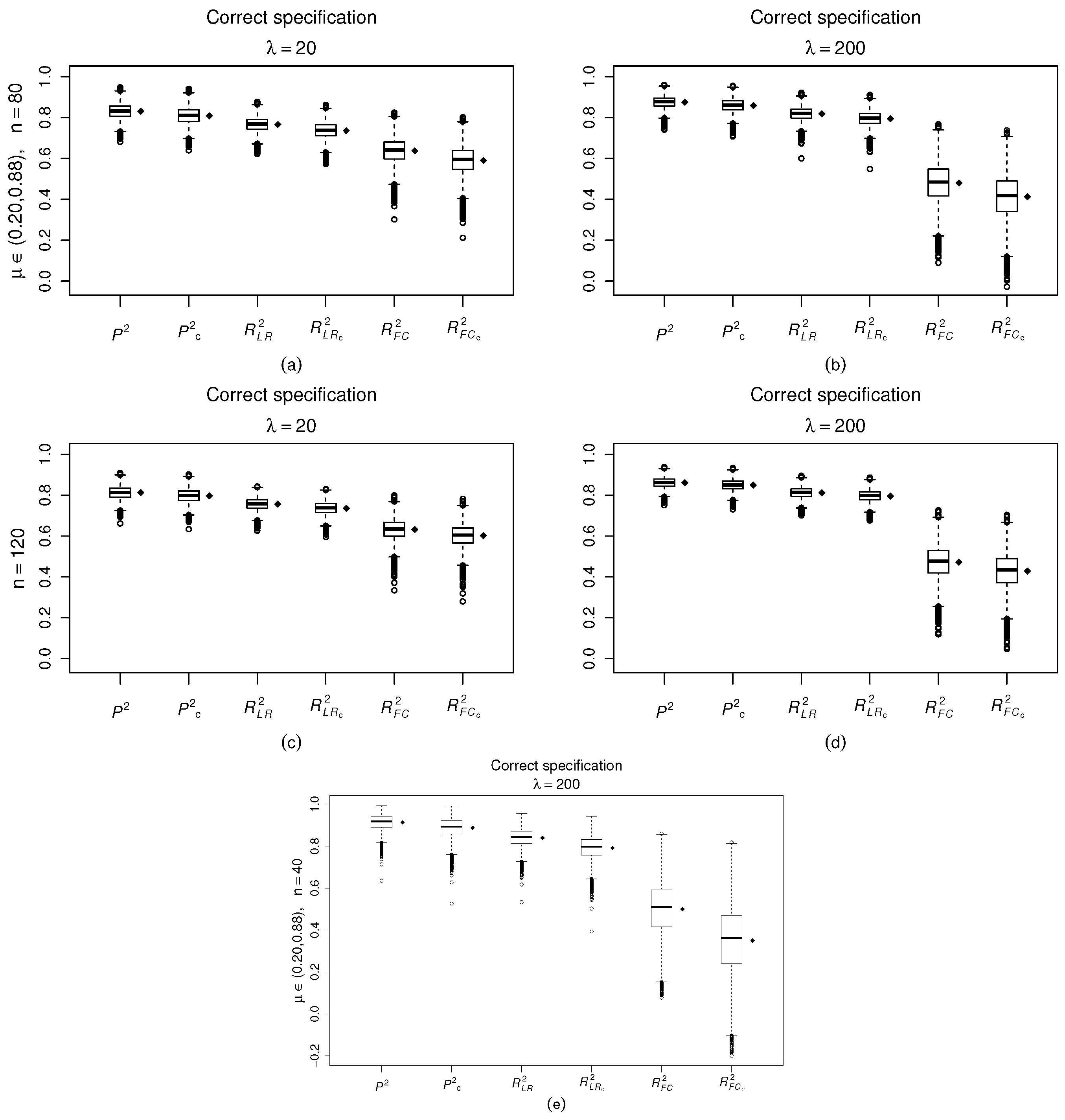
Table 3–Scenario 8).
Figure 4 supports this evidence. When
and the sample size increase, for example
and
, the values of
criterion tend to concentrate close to one, whereas the values of
and
tend to concentrate below
and
, respectively.
We shall focus on
,
Figure 4e the true intensity degree of nonconstant dispersion is close to 200, with
and
, whereas
with
and
that is a substantial distortion of the true intensity degree of nonconstant dispersion. Indeed, it is a substantial distortion of the true variance of the response observations.
Since the
-like criteria, select the model that can better explain the variability of the response, it is plausible that these measures present lower values when the distortions between the true and estimated variances of the response variable are so large. Please note that the
takes several values smaller than
and the
even takes negative values whereas overall the values of
are greater than
(
Figure 4e). Additionally, in this sense the
criterion proved to be more rigorous than the
criterion. This is a strong evidence that models with small
and high
values are worthy of further investigation. Indeed, the best fitted model should display high and close values of the three criteria and of their penalized versions.
3.3. Nonlinear Setting
In what follows, we shall present Monte Carlo experiments for the class of nonlinear beta regression models. The numerical results were obtained using the following beta regression model as data generating processes:
,
and
were kept fixed throughout the experiment. Here we use the starting value scheme for the estimation by ML proposed by [
23]. The precision and the sample size are respectively
,
. Additionally,
that yields
To evaluate the criterion performance on account of nonlinearity negligence, we consider the following model specification:
. All results are based on 10,000 Monte Carlo replications and for each replication.
We evaluated the behavior of the statistics both under model misspecification and under model correct specification. The results displayed in
Table 4 reveal that all statistics present values smaller when the model is missspecified. For example, fixing the precision value of
, for
, we have values of
,
and
equal to
, respectively. For
and
the values of the statistics are
and
, respectively. We simulated other nonlinear patterns to the sub-model mean predictor, and in some simulations the three criteria did not present smaller values of the feasible linear model than to the nonlinear model correctly specified.
5. Conclusions and Future Work
In this paper, we develop the criterion based on the PRESS-like machine learning tool for the class of beta regression models. We presented results of Monte Carlo simulations carried out to evaluate the performance the criterion and of the versions and of the criterion, under correct and incorrect model specifications. We consider different scenarios, including omission of covariates, negligence of varying dispersion and misspecification of nonlinearity. Two applications using real data were performed.
Both the simulation results and applications yield important conclusions. When the mean response is scattered on the standard unit interval, the and coefficients perform similarly well, and both enable to identify usual model misspecification. On the other hand, it is noteworthy that when the response values are close to one or zero the criterion outperformed the -like criteria in identifying problems on the model-fitting. Generally, these behaviors are related to influential observations and appropriated link functions for each range of response on standard unit interval. We notice that the log–log function models yield the best fits when the response is closer to zero, whereas the complementary log–log models yield the best fits when the response values are closer to one. These last conclusions were only supported by the criterion, but proved by the residual and influence analyses and by inference results. Another important conclusion is the poor performance of the criterion for beta regression models when the response is close to one of the standard unit interval boundaries. The outperforms the in identifying problems on the model variability on these ranges of the response variable. This conclusion is supported by the normal probability plots with simulated envelopes used in the real application.
Our proposed criterion proved to be very successful, since it selects the same models selected by the residual analysis, by the influence diagnostics and inference results. Despite this fact the normal probability plots with simulated envelopes reveal that questions about the model variability or the response distribution must be accessed the -like criteria.
Therefore, to the class of beta regression models the best strategy to select the best model to fit a dataset is jointly used the and criteria. When the two criteria being simultaneously close to one, better shall be the fitted model.
Further work will be devoted to the theoretical properties of the
statistic, and revisited statistical analysis, including post-Hoc analysis [
26,
27,
28] with the Tukey’s honestly significant difference test, and their
p-values adjusted via false discovery rate [
29] to highlight the existence of significant differences between the proposed and classical algorithms.


