Thermoplastic Composites: Modelling Melting, Decomposition and Combustion of Matrix Polymers

Abstract

In thermoplastic composites, the polymeric matrix upon exposure to heat may melt, decompose and deform prior to burning, as opposed to the char-forming matrices of thermoset composites, which retain their shape until reaching a temperature at which decomposition and ignition occur. In this work, a theoretical and numerical heat transfer model to simulate temperature variations during the melting, decomposition and early stages of burning of commonly used thermoplastic matrices is proposed. The scenario includes exposing polymeric slabs to one-sided radiant heat in a cone calorimeter with heat fluxes ranging from 15 to 35 kW/m². A one-dimensional finite difference method based on the Stefan approach involving phase-changing and moving boundary conditions was developed by considering convective and radiative heat transfer at the exposed side of the polymer samples. The polymers chosen to experimentally validate the simulated results included polypropylene (PP), polyester (PET), and polyamide 6 (PA6). The predicted results match well with the experimental results.

1. Introduction

Fibre-reinforced thermoplastic composites are increasingly being used as engineering materials for the automotive, construction and packaging sectors. The thermoplastic nature of the polymeric matrix makes them easy to be repaired by remoulding and recyclable. The disadvantage, however, is that thermoplastics have lower thermal stabilities than thermosets, restricting their usage in load-bearing structures. On exposure to heat, they undergo melting, decomposition and ignition, depending on the external heat flux. When held in vertical orientation, thermoplastics have a tendency to melt drip, which depending on the temperature could result in flaming drips, and hence may aid in the propagation of the fire. Melting also results in the deformation of the polymer. Many researchers, including ourselves, have tried to understand the melt dripping of thermoplastic polymers through laboratory and modelling work [1,2,3,4]. It was demonstrated that the melt dripping is a combined effect of physical melting and polymer decomposition, which results in a decrease in the viscosity of the molten drops [3]. The effect of fire and heat on melt dripping was also observed, where it was observed that the behaviour was quite different from pure melt dripping [3]. The temperature measurements of the molten drops and their thermal analytical studies gave an insight into the effect of external heat on the melting behaviour and prediction of the degree of degradation in the molten polymer [4]. However, in a horizontal orientation and contained situation, polymer melt will not escape from the containment region. This typical problem is called the Stefan problem involving solid–liquid phase change, with reference to the early work of Wisniak and Stefan [5], and is the subject of this study.

Modelling heat transfer within polymeric materials dates back to the mid-1940s; many models have been developed since then to simulate the burning behaviours of non-charring polymers [6,7] and charring polymers [8,9,10,11,12]. It is difficult to find in the literature a model that can describe all types of polymeric materials, as modelling differences exist among them. For example, non-charring polymers can be modelled using theory similar to flammable liquids. In contrary, the thermal response of charring polymers is the result of a complex interplay of chemistry, heat and mass transfer.

Polymers such as PP, PA6, and PET are non-charring polymers. Non-charring polymers change into gas volatiles during degradation reactions, leaving little or no char residues [13]. The solid phase of non-charring polymers can be divided into two layers. The upper layer is the degradation layer, in which degradation reactions occur. Gas volatiles are produced in this layer, which escapes to the air from the degradation layer through the surface. During this process, the mass flux of gas volatiles is determined by several properties, such as permeability, porosity and internal pressure. The bottom layer is a virgin polymer. Thus, the heat transfer through the material can be modelled using a theory similar to flammable liquids [7]. In the case of limited heat flux (<20 kW/m²), the heat transfer can be modelled by only using the heat conduction equation. However, as soon as the heat flux becomes more intense, the material decomposes and its internal structure is altered due to chemical reactions [14]. Thermal decomposition involves complex different physical and chemical processes taking place at the same time [15]. The degradation of materials is an endothermic process in which the energy input (activation energy) must be sufficient to break chemical bonds [12]. Hence, to theoretically model decomposition, comprehensive modelling involving a chemical kinetic scheme coupled with the conservation equations for the transport of heat and/or mass are required [16].

This study investigates the melting, decomposition and ignition behaviours of three thermoplastic polymers, polypropylene (PP), polyamide 6 (PA6) and polyethylene terephthalate (PET), upon exposure to a radiant heat on one surface only in a cone calorimeter, and the others being insulated so that there can be assumed a one-dimensional heat transfer within the sample from the top to the bottom. A sensitivity analysis [17] was performed to determine the thermophysical properties that have the most significant influence on the melting process of the studied thermoplastic polymers. The cone calorimeter experimental results obtained are used to validate the numerical model results utilising Matlab software. Using ignition theory, the temperature variations in the polymer during ignition could also be simulated.

2. Theoretical Model

A mathematical model was developed to simulate the melting behaviour of a horizontally oriented thermoplastic polymer slab in a cone calorimeter, where only the top surface is subjected to heat and all other sides are insulated. The model incorporates a moving boundary condition which enhances the standard heat transfer situation describing the Stefan phase change problem. This approach is based on the modelling work describing the process of the melting of ice by Kurscher et al. [18]. In addition to this, the model is further enhanced by introducing the capability of predicting the piloted ignition based on the Lyons approach, described by his equation based on the heat capacity and heat of gasification per unit mass of volatile [19].

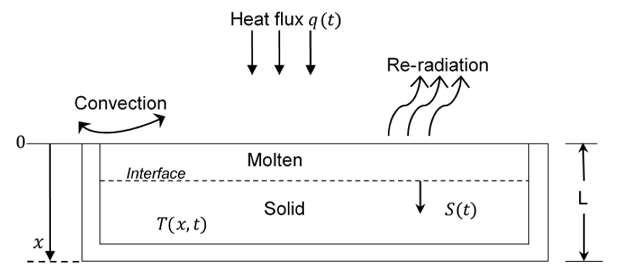
2.1. Heat Transfer Model with Moving Boundary Condition

2.1.1. Theoretical Approach

To develop a mathematical model for a horizontal thermoplastic polymer slab under an incident heat flux supplied by the cone calorimeter, the different heat transfer processes occurring are schematically shown in Figure 1. The model was idealised as a one dimensional process through the thickness with incident heat flux $q\left(t\right)$ applied only to the top exposed surface and no heat transfer taking place in other directions. Gradually, as the surface begins to melt, the interface (boundary region) with the solid polymer moves. This moving boundary condition is typical of the Stefan phase change problem. Due to the number of parameters and the complexity of the boundary conditions that need to be considered, the balance equation describing the situation is solved numerically to determine an approximate solution of the temperature distribution $T\left(x, t\right)$ through the thickness of the slab. The numerical method used to approximate the differential equations is the Finite Difference Method (FDM), embedded in MATLAB software by developing an appropriate program code. The molten–solid interface temperature is assumed to be the temperature $T_m$ of pure melting or melting plus partial decomposition or the ignition temperature when the thermoplastic sample catches fire.

The model developed includes a series of assumptions, these being: (1) once the surface temperature reaches the decomposition temperature $T_p$, the resultant products will immediately volatilise and be ignited by the ignition source, i.e., the ignition temperature $T_{ign}$ is assumed to be the same as the decomposition temperature $T_p$; (2) the decomposition process only takes place at the upper layer and there will be no mass transportation within the polymer; (3) the thickness of the interface layer between the melt and the solid phases is zero while in each phase the polymer’s specific heat and thermal conductivity increase with increasing temperatures [14,20]; thus, the thermal properties in the two different phases are assumed to be different, and the temperature gradient in the melt phase would be lower than that in the solid layer; and (4) only one-dimensional, through thickness, heat transfer is considered, and except for the upper surface, the other sides are treated as insulated.

Since this process concerns a phase change, the phase change material has a constant melting temperature $T_m$ and latent heat $H_L$. Each phase has a thermal conductivity, $k_L$ or $k_S$, and specific capacity, $c_{p_L}$ or $c_{p_S}$, which are phase-wise constant but with $k_L\ne k_S$; and $c_{P_L}\ne c_{P_S}$. The subscripts ‘$L$’ and ‘$s$’ denote the liquid and the solid phase. Furthermore, it is assumed that heat is transferred isotropically (i.e., equal in all directions). The interface separating each phase is assumed to be sharp, planar, without surface tension and of zero thickness [15,21,22,23,24].

2.1.2. Model Description

The heat transfer by the conduction of the model shown schematically in Figure 1 is described mathematically by the balance Equation (1), to be solved for $T\left(x, t\right)$ [1,25]:

$$\rho \left(T\right)C_p\left(T\right)\frac{\partial T\left(x,t\right)}{\partial t}=k\left(T\right)\frac{\partial T^2\left(x,t\right)}{\partial x^2}+\dot{m} (H_c-H_L-H_g)$$

(1)

where $\rho \left(T\right)$ is the polymer density, $C_p\left(T\right)$ is the polymer-specific heat capacity, $k\left(T\right)$ is the polymer-specific conductivity, $\dot{m}$ is the rate of mass phase change, $H_L$ is the latent heat of melting, $H_g$ is the enthalpy of pyrolysis and $H_c$ is the enthalpy of combustion.

The boundary condition for an imposed flux $q\left(t\right)$ is:

$$-k\left(T\right)\frac{\partial T\left(0,t\right)}{\partial x}=q\left(t\right),-k\left(T\right)\frac{\partial T\left(L,t\right)}{\partial x}=0$$

$$-k\left(T\right)\frac{\partial T\left(0,t\right)}{\partial x}=q\left(t\right),-k\left(T\right)\frac{\partial T\left(L,t\right)}{\partial x}=0$$

The thermoplastic polymer sample is composed of two phases: liquid and solid phase separated by an interface $S\left(t\right)$; see Figure 1, which illustrates the model description. The polymer slab is isolated on its sides to have a one-dimensional slab with a thickness $L$ where the phase change process, decomposition and ignition are undergoing. For liquid phase and solid phase, Equation (1) becomes, respectively [4,18,26]:

$$\frac{\partial T\left(x,t\right)}{\partial t}={\alpha }_l\frac{{\partial }^{2}T\left(x,t\right)}{\partial x^2},\hspace{0.17em}\hspace{0.17em}0<x<S\left(t\right)\left(liquid phase\right)$$

(2)

$$\frac{\partial T\left(x,t\right)}{\partial t}={\alpha }_s\frac{{\partial }^{2}T\left(x,t\right)}{\partial x^2},\hspace{0.17em}\hspace{0.17em}S\left(t\right)<x<L\left(solid phase\right)$$

(3)

where,

$${\alpha }_l=\frac{k_l}{\rho c_l}\hspace{0.17em}\hspace{0.17em}and\hspace{0.17em}\hspace{0.17em}{\alpha }_s=\frac{k_s}{\rho c_s}$$

The subscript ‘$l$’ and ‘$s$’ denote the liquid or the solid phase, and ${\alpha }_l$ and ${\alpha }_s$ are the diffusivity in the liquid phase and solid phase, respectively. The expression of the velocity $\dot{S}$ of the interface $S\left(t\right)$ is proportional to the sudden change in the heat flux across the interface liquid/solid, and it is given by:

$$\rho \dot{S}\left(t\right)H_L=k_s\left(T\right)\frac{\partial T\left(S\left(x\right),t\right)}{\partial x}-k_l\left(T\right)\frac{\partial T\left(S\left(x\right),t\right)}{\partial x},\hspace{0.17em}\hspace{0.17em}S\left(t\right)<x<L$$

(4)

where is the sample thickness and $\dot{S}\left(t\right)$ is the velocity of the moving interface. The material is initially solid at an ambient temperature $T_a$. Since an incident flux $q\left(t\right)$ is applied at $x=0$, melting occurs when $T=T_m$, $T_m$ being the melting temperature. At the insulated side $x=L$, the heat transfer by conduction is equal to zero where the temperature is assumed to be at ambient temperature $T_a$. When $t>0$, the liquid state of the polymer occupies the space $\left[0; S\left(t\right)\right]$ if $T=T_m$, while the solid state occupies $\left[S\left(t\right); L\right]$ if $T<T_m$. This leads to the two-phase Stefan problem. The initial, the interface and the boundary conditions are:

Initial conditions:

$$S\left(0\right)=0\left(material initially solid\right)$$

and

$$T\left(x,0\right)=T_a,\hspace{0.17em}\hspace{0.17em}for\hspace{1em}0<x<L.$$

Interface conditions:

$$T\left(S\left(t\right), t\right)=T_m\hspace{0.17em}\hspace{0.17em}for\hspace{1em}t>0$$

and

$$\rho \dot{S}{H}_L=k_s\left(T\right)\frac{\partial T\left(S\left(x\right),t\right)}{\partial x}-k_l\left(T\right)\frac{\partial T\left(S\left(x\right),t\right)}{\partial x},\hspace{0.17em}\hspace{0.17em}for\hspace{1em}t>0$$

where,

$$\dot{S}=-\beta \frac{\partial T\left(S\left(x\right),t\right)}{\partial x}$$

(5)

and

$$\beta =\frac{k_s-k_l}{\rho H_L}$$

Boundary conditions:

$$T\left(0<x<S\left(t\right),t\right)=T_m or T_{ign},\hspace{0.17em}\hspace{0.17em}for\hspace{1em}t>0,$$

and

$$T\left(l,t\right)=T_a$$

2.2. Model Incorporating Ignition Behaviour

2.2.1. Theory

Once the surface reaches the ignition temperature, $T_{ign}$, the polymer ignites. $T_{ign}$ is defined here as [19]:

$$T_{ign}\approx {\left[\frac{T_0{h}_g}{C_0}\right]}^{\frac{1}{2}}$$

(6)

where $C_0$ is the heat capacity of the solid at $T_0$ = 298 K and $h_g$ is the heat of gasification per unit mass of volatile.

At ignition, the enthalpy of combustion ($H_c$) and gas ($H_g$) are added to the system in addition to the heat transfer by radiation and convection between the flame and the exposed side of the polymer sample. Thus, the boundary conditions and the temperature distribution changes are almost instantaneous on the exposed face. This process is incorporated in the model and program. The programming code developed with Matlab implements the behaviour post ignition, and thus predicts the temperature profiles after this event.

2.2.2. Numerical Method to Predict Temperature Behaviour

In order to estimate the solutions to the problem described previously, a set of algorithms were developed. These algorithms enable solutions to be determined numerically. The heat equation is associated with the moving boundary due to a phase change by melting for each time step [13]. The process involves updating the temperature distribution using an explicit scheme of the Finite Difference Method (FDM) for the heat equation, as such:

$$\frac{T_i^{t+\Delta t}-T_i^t}{\Delta t}=\alpha \frac{T_{i-1}^t-2T_i^t+T_{i+1}^t}{{\left(\Delta x\right)}^2}$$

(7)

The space discretisation is $\left(0, \Delta x, 2\Delta x,\dots , n\Delta x\right)$ and at time $t$ with $L=n\Delta x$ be the greatest discretisation point below $S\left(t\right)$ and the vector $T\left(t\right)={\left[T_1\left(t\right)···T_n\left(t\right)\right]}^T$ as the temperature vector in discretisation points: $T\left(t\right)={\left[T\left(0,t\right)···T\left(n\Delta x,t\right)\right]}^T$.

By separating terms with $T\left(t\right)$ from terms with $T\left(t+\Delta t\right),$ Equation (6) can now be solved for $T\left(t+\Delta t\right)$.

Subsequently, the boundary state is updated and an explicit scheme of the Finite Difference Method (FDM) in Equation (5) is thus described:

$$\frac{S_x^{t+\Delta t}-S_x^t}{\Delta t}=-\beta \frac{T_x^t-T_{x-\Delta x}^t}{\Delta x}$$

Now, the space discretisation is $\left(0, \Delta x, 2\Delta x, . . . , n\Delta x\right)$ and at time $t,$ if $x_0$ is the discretisation point below $S\left(t\right)$. The finite difference approximation of the derivative of $T\left(S\left(t\right),t\right)$ between $(x_0-\Delta x)$ and $x_0$ is given by:

$$\frac{\partial T\left(S\left(x\right),t\right)}{\partial x}\approx \frac{T\left(x_0, t\right)-T\left(x_0-\Delta x,t\right)}{\Delta x}=\frac{T_{x_0}^t-T_{x_{0-\Delta x}}^t}{\Delta x}$$

(8)

The choice of discretisation points in the calculation of the finite difference in the boundary moving step is crucial for stability issues. The most natural choice for the space discretisation points would be the boundary value and the one before the boundary, but this choice leads to potentially unstable values of the derivative of the temperature $T$ with respect to $x$. Therefore, the two last discretisation points before the boundary need to be used to improve the approximation of the derivative.

3. Materials and Methods

3.1. Materials and Sample Preparation

The following commercially available polymers were used:

• Polypropylene (PP), Moplen HP516R, LyondellBasell, Warrington, UK;
• Polyamide 6 (PA6), Technyl C 301 Natural, Rhodia, Saint Frons, France;
• Polyethylene terephtalate (PET, polyester) received from Fibre Extrusion Technology, Leeds, UK.

From polymer chips of PP, PA6 and PET, plaques were prepared by a melt-pressing process, where chopped polymer chips were transformed into 150 mm × 150 mm × ~3 mm-sized plaques using high temperature (melting temperature of the polymer) and pressure (20 kg/cm²) for 3 min, followed by sudden cooling. The polymer plaques were then cut into small specimens of the required sizes.

3.2. Thermal Analysis

In order to obtain the fundamental properties of the polymers, thermogravimetric analysis was performed on an SDT 2960 simultaneous DTA–TGA instrument (TA Instruments, Elstree, Hertfordshire, UK) from room temperature to 600 °C using 15 ± 1 mg samples heated at a constant heating rate of 10 °C/min in both air and nitrogen flowing at 100 ± 5 mL/min. Additionally, the glass transition temperatures or melting temperatures of all polymers were measured using differential scanning calorimetry (DSC) (TA Instruments, Elstree, Hertfordshire, UK) at 10 °C/min in flowing N₂ (100 mL/min).

3.3. Measurement of Temperatures of Horizontally Oriented Samples Exposed to Radiant Heat in a Cone Calorimeter

A cone calorimeter apparatus (Fire Testing Technology Ltd., East Grinstead, UK) was used to investigate the melting, decomposition and ignition behaviours of horizontally oriented polymer slabs, keeping 25 mm distance between the heater and the sample surface as specified in ISO 5990 [27]. However, in this work spark ignition was not used and heat fluxes were kept low enough to measure temperature changes during the melting and initial stages of the burning of polymers. Three constant incident heat fluxes, 15, 25 and 35 kw/m², were applied only on the top surface of the polymeric samples, the other sides being insulated by a ceramic woven such that it is assumed that one-dimensional heat transfer occurs. Four K-type thermocouples were inserted in each sample, two on top of the surface and two on the back surface of samples. A schematic description of the cone calorimeter and its temperature measurement setup is shown in Figure 2.

4. Results and Discussion

4.1. Thermal Analytical Results

Differential thermal analysis (DTA, temperature difference between sample and reference versus temperature) or differential scanning calorimetry (DSC, difference in the amount of energy required to maintain the sample and reference at the same temperature versus temperature) is a commonly used technique to detect thermally induced physical and chemical transitions in a sample, whereas thermogravimetry (TGA, mass loss versus temperature) provides information about chemical transitions only. DTA curves for all samples in air and nitrogen are shown in Figure 3. Analysed results from TGA and DSC studies are presented in

Table 1. Analysis of thermal behaviour (DTA-TGA) of polymers in air and nitrogen atmosphere (values reported in parenthesis) of polymers.

Polymer	TGA Analysis		Glass Transition Temp. b (°C)	Melting Temp. b (°C)
	TOnset a	DTG Maxima (°C)
PP	274 (415)	367 (459)	−26	172
PA6	372 (375)	434, 458 (456)	54	225
PET	378 (397)	429, 446, 538 (439)	68	256

Note: ^a T_Onset = onset of decomposition temp, where 5% mass loss occurs; ^b measured by DSC.

. While both DTA and DSC provide similar information regarding temperature-dependent chemical and physical changes, power-compensated DSC, which uses a feedback loop to maintain the sample at a set temperature while measuring the power needed to do this against a reference furnace, allows for very precise control of temperature, resulting in very accurate (up to two decimal point) measurements. Since the polymers used in this work are of commercial grade and may contain some impurities, the glass transition and melting temperatures are reported as integers in Table 1.

As can be seen from Figure 3, the atmosphere has no effect on physical transitions, seen as endothermic peaks related to the melting of the polymers, whereas the decomposition process is significantly affected in terms of temperature ranges as well as from endothermic DTA transitions in nitrogen to exothermic transitions in air. Moreover, in nitrogen, there is a single mass loss step, whereas in air there is an additional char oxidation step for each polymer. The temperature at the maximum mass loss from each step, represented by the peak maximum of each derivative thermogravimetric (DTG, not shown here) peak, is given in Table 1. In PP, the onset of decomposition temperature, T_Onset (taken as the temperature where 5% mass loss occurs), in air is 274 °C, whereas in N₂ it is 415 °C. The difference in the thermal decomposition behaviour of PP in air and N₂ atmospheres is well known and discussed in detail in the literature [28]. In PA6 and PET, while T_Onset in air is reduced compared with that in nitrogen, the difference between the two is much less than in PP. This information is important to understand the surface temperature changes in samples exposed to cone calorimetric tests, to be discussed in the following sections. Since the cone experiments are performed under room conditions, the exposed surface is in an air environment at the beginning of the experiment. The temperature through the thickness of the sample is vitiated. As the temperature on the surface increases and ignition occurs, oxygen is consumed and the atmosphere becomes vitiated. Hence, until T_Onset, the surface temperature in the experiment can be related to air atmosphere. For glass transition and melting point measurements, separate DSC experiments were performed in nitrogen, and the results are used for the discussion in the following sections.

4.2. Input Parameter and Sensitivity Analysis

The material properties of the polymers used as input parameters were taken from the literature and are listed in

Table 2. Thermal and physical properties of different polymers at 25 °C [29] used for heat transfer modelling.

Polymer	Thermal Conductivity, k (W/m·k)	Specific Heat Capacity, cp (J/kg·k)	Density, ρ (kg/m3)
PP	0.12	1622	910
PA6	0.15	1172	1350
PET	0.24	1502	1177

.

It is well known that the specific thermal conductivity k and the specific heat capacity c_p vary with temperature and can influence the behaviour of the process. Hence, a sensitivity study was carried out on these parameters to build confidence in the model and justify the use of the parameters. Therefore, to understand the effect of these parameters, the model was run in MATLAB using changes in the values of thermal conductivity k and heat capacity C_p to obtain temperature profiles at the surface of PP, subjected to 35 kW/m² external heat flux on the surface of the polymer slab. The values of k (0.12 W/m·k) and C_p (1622 J/kg·k), as given in Table 2, were considered for performing the sensitivity analysis. The first step was to vary by k by +/−10% and c_p up to +/−30% and thus observe the variation in the predicted temperature values as a function of time.

A sensitivity analysis was carried out based on the ‘normalised sensitivity function’, which indicates the ratio between the change in percentage of k or C_p as an input and the change in percentage of the temperature profile as an output. The sensitivity function is defined as [2]:

$$S\left(T,k\right)=\frac{dT}{dk}·\frac{k}{T}$$

(9)

and

$$S\left(T,C_p\right)=\frac{dT}{d{C}_p}·\frac{C_p}{T}$$

(10)

where k, C_p, $\frac{dT}{dk}$ and $\frac{dT}{d{C}_p}$ are, respectively, the heat conductivity, the heat capacity, the temperature gradient related to the conductivity and the temperature gradient related to the heat capacity. The results obtained from the sensitivity analysis are shown in Figure 4. The results indicate that the surface temperature of the polymer increases or decreases when thermophysical parameters, specific thermal conductivity (k) and specific heat capacity (C_p) increase or decrease.

The specific thermal conductivity (k) influences the output temperature profile more than the specific heat capacity. Figure 4 shows that the ratio given by the sensitivity analysis is around 0.2 for k and C_p, which means, for example, the change of 10% in k or C_p induces a change of approximately 2% in the temperature profile. Though these values are temperature dependent, owing to the non-availability of such data for temperatures of interest in this study, a constant value at 25 °C taken from ref [29] was used.

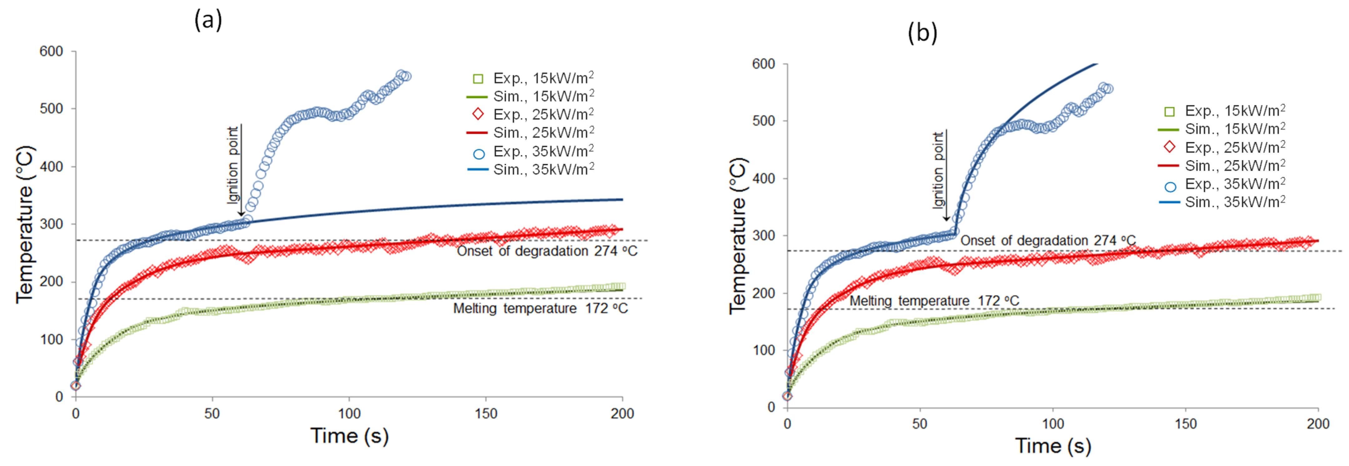
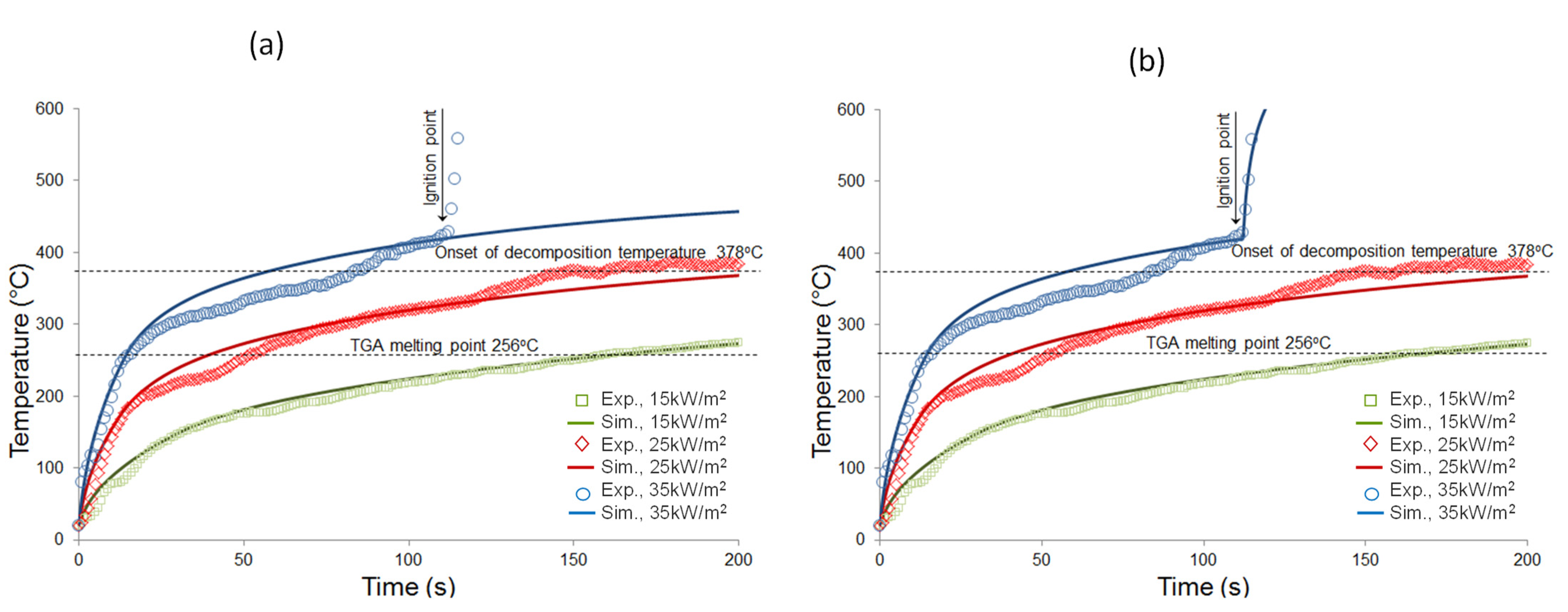
4.3. Simulation Results

Using the programming code designed with Matlab, the predicted temperature profiles are shown in Figure 5, Figure 6 and Figure 7. Figure 5a and Figure 7a show the simulated profile temperatures using Matlab without the implementation of the condition of the ignition, while Figure 5b and Figure 7b show the predicted profile temperatures with the ignition condition based on Equation (6). Additionally, shown in the same figures are the melting and T_Onset temperatures measured by DSC and TGA, respectively. In order to validate the model, the experimental results are also shown as solid lines in Figure 5, Figure 6 and Figure 7.

All curves in Figure 5, Figure 6 and Figure 7 show that the surface temperature of each polymer is not higher than the theoretical melting temperature of the polymer at an incident heat flux of 15 kW/m². When the heat flux is increased to 25 kW/m², PP’s temperature is higher than the theoretical melting temperature after 150 s and very close to the T_Onset in air (274 °C), indicating that decomposition may have started. At 35 kW/m², the temperature rises very quickly above the T_Onset and the sample ignites when the surface temperature approaches ~300 °C (Figure 5), after which the temperatures rises very quickly to a flaming temperature, i.e., >500 °C. In PA6 and PET, temperatures at 25 kW/m² are between the theoretical melting temperature and decomposition temperature. At an incident heat flux of 35 kW/m², PA6 does not reach the theoretical decomposition temperature even if the polymer ignites after 100 s. PET, however, ignites soon after reaching 425 °C (Figure 7) at 110 s exposure time.

The simulated results from the models described in Section 2.1, shown as open circles in Figure 5a and Figure 7a, show good agreement with experimental temperatures until ignition occurs. However, upon incorporating the ignition criteria in the model (Section 2.2), the model also simulates the ignition criterion in good agreement with the experimental results, as seen from Figure 5b and Figure 7b. It must, however, be noted that the thermophysical parameters used to build the numerical model are taken from the literature and despite the fact that they vary with temperature, their accuracy is difficult to establish [30]. Another issue is that, experimentally, the bottom surface temperature of the sample was relatively easy to measure compared with the top surface temperature exposed to the heat flux because of the difficulty to keep the thermocouples stable, as they can easily move into the molten thermoplastic samples. Despite these shortcomings, the model simulations are close to the experimental values. These results also show the speed at which these materials can melt, providing an indication on the development of pool molten thermoplastic polymer formation, which often leads to polymer degradation and ignition when the incident heat flux is high enough [4,31].

5. Conclusions

A one-dimensional mathematical model of heat transfer by conduction through the thermoplastic polymers was developed, which has the capability of accounting for the melting process to include degradation, along with the prediction of surface ignition not previously described. All these phenomena are described by a balance equation, which is a nonlinear Partial Differential Equation (PDE). Approximated numerical solutions are obtained using the Finite Difference Method (FDM) for the one-dimensional (1D) domain, Stefan phase change and moving boundary problem statement. Key parameters such as specific thermal conductivity, heat capacity, density and latent heat for three thermoplastic polymers studied here (PP, PA6 and PET) were taken from the literature. To understand the effect of input parameters on the simulated results, a sensitivity analysis was undertaken to find out which parameter has the greatest influence on the model behaviour.

The experimental temperature profiles of the thermoplastic materials exposed to three different heat fluxes (15, 25 and 35 kW/m²) in a cone calorimeter were used to validate the model. A good agreement between the predicted and experimental temperature profiles shows the effectiveness of the model. However, the model could be further improved by incorporating changes to specific heat capacity and conduction as a function of temperature, along with extending to a two- or three-dimensional approach to the problem.

References

1. Zhang, J.; Shields, T.J.; Silcock, G.W.H. Effect of melting behaviour on upward flame spread of thermoplastics. Fire Mater. 1997, 21, 1–6. [Google Scholar] [CrossRef]
2. Ohlemiller, T.J.; Butler, K. Influence of Polymer Melt Behaviour on Flammability 2000. Available online: https://nvlpubs.nist.gov/nistpubs/Legacy/IR/nistir6588v1.pdf (accessed on 18 December 2020).
3. Kandola, B.K.; Price, D.; Milnes, G.J.; Da Silva, A. Development of a novel experimental technique for quantitative study of melt dripping of thermoplastic polymers. Polym. Degrad. Stab. 2013, 98, 52–63. [Google Scholar] [CrossRef]
4. Kandola, B.K.; Ndiaye, M.; Price, D. Quantification of polymer degradation during melt dripping of thermoplastic polymers. Polym. Degrad. Stab. 2014, 106, 16–25. [Google Scholar] [CrossRef]
5. Wisniak, J. Josef Stefan: Radiation, conductivity, diffusion, and other phenomena. Rev. CENIC Cienc. Químicas 2006, 37, 188–195. [Google Scholar]
6. Di Blasi, C.; Crescitelli, S.; Russo, G.; Cinque, G. Numerical model of ignition processes of polymeric materials including gas-phase absorption of radiation. Combust. Flame 1991, 83, 333–344. [Google Scholar] [CrossRef]
7. Di Blasi, C. Modeling of solid- and gas-phase processes during thermal degradation of composite materials. Polym. Degrad. Stab. 1996, 54, 241–248. [Google Scholar] [CrossRef]
8. Di Blasi, C. Numerical simulation of cellulose pyrolysis. Biomass Bioenergy 1994, 7, 87–98. [Google Scholar] [CrossRef]
9. Criado, J.M.; Pérez-Maqueda, L.A. Sample controlled thermal analysis and kinetics. J. Therm. Anal. Calorim. 2005, 80, 27–33. [Google Scholar] [CrossRef]
10. Vyazovkin, S.; Wight, C.A. Isothermal and nonisothermal reaction kinetics in solids:  In search of ways toward consensus. J. Phys. Chem. A 1979, 101, 8279–8284. [Google Scholar] [CrossRef]
11. Henderson, J.B.; Wiebelt, J.A.; Tant, M.R. A model for the thermal response of polymer composite materials with experimental verification. J. Comp. Mat. 1985, 19, 579–595. [Google Scholar] [CrossRef]
12. Staggs, J.E.J. Ignition of char-forming polymers at a critical heat flux. Polym. Degrad. Stab. 2001, 74, 433–439. [Google Scholar] [CrossRef]
13. Di Blasi, C. Transition between regimes in the degradation of thermoplastic polymers. Polym. Degrad. Stab. 1999, 64, 359–367. [Google Scholar] [CrossRef]
14. Chartoff, R.C. Thermoplastic polymers. In Thermal Characterization of Polymeric Materials, 2nd ed.; Turi, E.A., Ed.; Academic Press: New York, NY, USA, 1997; pp. 621–625. [Google Scholar]
15. Stefan, J. Ueber die theorie der eisbildung, insbesondere uber die eisbildung im polaemeere. Ann. Der Phys. Chem. 1891, 42, 269–286. [Google Scholar] [CrossRef] [Green Version]
16. Nyazika, T.; Jimenez, M.; Samyn, F.; Bourbigot, S. Pyrolysis modelling, sensitivity analysis, and optimization techniques for combustible materials: A review. J. Fire Sci. 2019, 37, 377–433. [Google Scholar] [CrossRef]
17. Salva, N.N.; Tarzia, D.A. A sensitivity analysis for the determination of unknown thermal coefficients through a phase-change process with temperature-dependent thermal conductivity. Int. Commun. Heat Mass Transf. 2011, 38, 418–424. [Google Scholar] [CrossRef]
18. Kurschner, P.; Maki-Marttunen, T.; Vestergaard, S.; Wandl, S. Modelling and simulation of ice/snow melting. In Proceedings of the 22nd ECMI Modelling Week, Eindhoven, The Netherlands, 31 October 2008. [Google Scholar]
19. Lyon, R.E.; Quintiere, J.G. Criteria for piloted ignition of combustible solids. Combust. Flame 2007, 151, 551–559. [Google Scholar] [CrossRef]
20. Thompson, E.V. Thermal properties. In Encyclopedia of Polymer Science and Engineering; Mark, H.F., Ed.; John Wiley & Sons: New York, NY, USA, 1989; Volume 16, pp. 711–747. [Google Scholar]
21. Crank, J. Two method for the numerical solution of moving-boundary problems in diffusion and heat flow. Quart. J. Mech. Appl. Math. 1957, 10, 220–231. [Google Scholar] [CrossRef]
22. Crank, J. Fire and Moving Boundary Problem; Clarendon Press: Oxford, UK, 1984. [Google Scholar]
23. Poirier, D.; Salcudean, M. On numerical methods used in mathematical modelling of phase change in liquid metal. J. Heat Transf. 1988, 110, 562–569. [Google Scholar] [CrossRef]
24. Bradean, R.; Ingham, D.B.; Heggs, P.J. Stefan problem in blow moulding operations. In Mathematics of Heat Transfer; Tupholme, G.E., Wood, A.S., Eds.; Oxford Clarendon Press: Oxford, UK, 1998; pp. 89–96. [Google Scholar]
25. Ohlemiller, T.; Shields, J.; Butler, K.; Collins, B.; Seck, M. Exploring the role of polymer melt viscosity in melt flow and flammability behavior. In Proceedings of the Fall Conference of the Fire Retardant Chemicals Association, Ponte Vehdra, FL, USA, 15–18 October 2000. [Google Scholar]
26. Šarler, B. Stefan’s work on solid-liquid phase change. Eng. Anal. Bound. Elem. 1995, 16, 83–92. [Google Scholar] [CrossRef]
27. ISO 5660-1:2015. Reaction-To-Fire Tests—Heat Release, Smoke Production and Mass Loss Rate—Part 1: Heat Release Rate (Cone Calorimeter Method) and Smoke Production Rate (Dynamic Measurement); International Organization for Standardization: Geneva, Switzerland, 2015. [Google Scholar]
28. Zhang, S.; Horrocks, A.R. A Review of fire retardant polypropylene Fibres. Prog. Polym. Sci. 2003, 28, 1517–1538. [Google Scholar] [CrossRef]
29. Mark, J.E. (Ed.) Physical Properties of Polymers Handbook, 2nd ed.; Springer Science: New York, NY, USA, 2007; ISBN 978-0-387-69002-5. [Google Scholar]
30. Vyazovkin, S. Modification of the integral isoconversional method to account for variation in the activation energy. J. Compt. Chem. 2001, 22, 178–183. [Google Scholar] [CrossRef]
31. Onate, E.; Marti, J.; Ryzhakov, P.; Rossi, R.; Idelsohn, S.R. Analysis of the melting, burning and flame spread of polymers with the particle finite element method. Comput. Assist. Methods Eng. Sci. 2013, 20, 165–184. [Google Scholar]
Figure 1. Horizontal thermoplastic slab insulated at the sides.
Jcs 06 00027 g001
Figure 2. Schematic of the cone calorimetric setup for temperature measurements.
Jcs 06 00027 g002
Figure 3. TGA (left-hand ordinate) and DTA (right-hand ordinate) curves of (a) PP, (b) PA6 and (c) PET in air and nitrogen atmospheres.
Jcs 06 00027 g003
Figure 4. Change in surface temperature (%) versus time for PP when the thermal conductivity (k) or the heat capacity (Cp) changes by +/−10% up to 30%.
Jcs 06 00027 g004
Figure 5. Experimental and simulated surface temperatures of PP exposed to 15, 25 and 35 kW/m2 heat fluxes by (a) thermal model and (b) by incorporating ignition criteria.
Jcs 06 00027 g005
Figure 6. Experimental and simulated surface temperatures of PA6 exposed to 15, 25 and 35 kW/m2 heat fluxes by (a) thermal model and (b) by incorporating ignition criteria.
Jcs 06 00027 g006
Figure 7. Experimental and simulated surface temperatures of PET exposed to 15, 25 and 35 kW/m2 heat fluxes by (a) thermal model and (b) by incorporating ignition criteria.
Jcs 06 00027 g007