Four Point Flexural Response of Acrylonitrile–Butadiene–Styrene

Abstract

Acrylonitrile–Butadiene–Styrene (ABS) is a very significant and widely used amorphous thermoplastic that possesses high impact resistance, toughness, and heat resistance. Bending collapse is a predominant failure of polymeric structural members in the vehicle environment under angled and unsymmetrical collisions. Therefore, it becomes critical to investigate the flexural behavior of the ABS beam and find its energy absorption capabilities under a transverse loading scenario. Four-point bending tests were carried out at different strain rates and at two different span lengths to investigate the deformation behavior of ABS. This paper examines the influence of strain rate, friction coefficient, Generalized Incremental Stress-State MOdel (GISSMO) and Damage Initiation and Evolution (DIEM) damage models, yield surfaces, and the span length on the four-point flexural behavior of the ABS polymeric material. A Semi-Analytical material model (SAMP_1) in LSDYNA was utilized to numerically evaluate the behavior of ABS under four-point bending. From extensive investigative explorations, it was found that the flexural behavior of ABS is dependent upon the span length, loading strain rate, and friction coefficient between the specimen and the supports. The modeling of damage was successfully exemplified by using the inherent damage law of the SAMP-1 material model, GISSMO, and DIEM damage formulations.

1. Introduction

Amorphous thermoplastics such as Acrylonitrile–Butadiene–Styrene (ABS) have been used as a structural component in a wide range of engineering applications, such as automotive trim components, luggage applications, sea and land vehicles, and medical devices because they possess many excellent and highly desired material properties for a cost-effective structure. ABS material possesses high stiffness, high toughness, good impact resistance, and high compressive strength. Lightweight, durability, and cost effectiveness are also a driving force behind its widespread usage in all sectors. Therefore, it becomes necessary to study the behavior of this thermoplastic material rigorously under different loading strain rates and setup parameters to have better and deep understanding of their response to flexural loads. Understanding the non-linear behavior of thermoplastics subjected to instant multiaxial loadings is an increasing demand. Many studies have been conducted to find out the complex material behavior of thermoplastics to mechanical loadings. While the response of thermoplastics during low rate deformation is quite comprehensible and documented, there is still a high need to understand the response of thermoplastics under high rate deformation [1]. Due to the relative motions of molecular chains to each other, many contemporary thermoplastics can undergo extremely large plastic deformations [2]. Withstanding large plastic deformations makes thermoplastics well suitable for such specific engineering applications where good impact resistance is desired [3]. The material properties of thermoplastics are considerably dependent on temperature and strain rate [4]. The strain rate dependence can be explained by the identical motions of chains with the deformation rate [5]. In addition, dissimilar material behavior between tension and compression is observed in many thermoplastics. This shows that hydrostatic pressure plays a significant role in yield stresses [6]. In the literature, uniaxial tension and uniaxial compression stress–strain curves with various strain rates for different types of thermoplastics were found to reflect the strain rate and hydrostatic pressure effects on yield stresses [3,7,8].

For many years, a great deal of attention has been given to derive a constitutive material model for the characterizaion of strain rate and pressure dependent material behavior of thermoplastics. Although many experimental and theoretical studies have been dedicated to obtain the reliable consititutive material model for the identification of strain rate and pressure-dependent material behaviors of thermoplastics when they are subjected to multiaxial mechanical loads such as impact, three-point bending, and four-point bending, developing the constitutive material model has been currently a major concern [9,10,11,12,13,14,15,16]. The most proposed material models are associated with specifying the strain rate-dependent material behavior of thermoplastics rather than defining their pressure-dependent material behaviors, but those material models have been derived based on experimental data measured from either tension or compression tests conducted on various thermoplastics over a wide range of strain rates. Nevertheless, the mechanical response of thermoplastics to only tensile or only compressive loads does not reflect their material behavior subjected to multiaxial loads dictating tension, compression, and shear stress states simultaneously. Particularly, understanding the high strain rate response of thermoplastics has been currently under investigation, since thermoplastics that are subjected to high rate deformations show an intrinsic failure mechanism, and the reason behind it has not been comprehended at present. A more fundamental understanding of the high strain rate response behavior of thermoplastics and a more complex material model is highly needed [17,18,19].

In addition, many attempts have been made to characterize the dissimilar material behavior of thermoplastics in tension and in compression. Depending on the modifications of Von Mises and Tresca yield criteria, many researchers have come up with several new yield theories. It was pointed out that the pressure-modified VonMises criterion was well satisfied with the determination of pressure-dependent yield behavior of thermoplastics [20]. The pressure-modified Tresca and Mohr–Coulomb criteria were addressed to characterize the pressure-dependent yield behavior of thermoplastics [19,21]. Nevertheless, both the pressure-modified Tresca and Mohr–Coulomb criteria are not well satisfactory for the identification of dissimilar material behavior of thermoplastics between tension and compression [18].

Due to the limitations in understating the strain rate-dependent material behavior of thermoplastics and possessing a reliable material model for the characterization of strain rate dependency and pressure dependency effects on the material behavior of thermoplastics, an experimental investigation and numerical validation with the help of semi-empirical material models available in finite element codes are preferred for the determination of material behavior of thermoplastics subjected to multiaxial loads such as four-point bending. In this study, four-point bending tests were conducted on ABS (Acrylonitrile–Butadiene–Styrene) amorphous thermoplastic material under distinct testing speeds. From the experimentally obtained stress–strain curves for all three stress states, tension, compression, and shear, the effect of test speed and span length on the yield stress of ABS was investigated. Additionally, the numerical simulations using an explicit solver, LSDYNA were also performed for a given test speed to document the effect of static and dynamic friction coefficients between specimen and supports on the yield behavior of ABS. Mat_SAMP-1 (Semi Analytical Model for Polymers) in LSDYNA was recently developed particularly for polymers and it is capable of handling various loading cases such as multiaxial and damage [22,23]. One of the most promising aspects of this material model is to allow us to introduce the experimentally determined uniaxial tension, uniaxial compression, and shear stress–strain curves to the model in terms of yield stresses and corresponding plastic strains [24]. Therefore, the Mat_SAMP-1 material model was utilized in our simulations and the corresponding plastic strains as a function of yield stresses were assigned to the model successfully. Numerically obtained load versus displacement curves for various test speeds were compared to the experimental findings, and very good agreements were observed between the numerical and experimental results. From the good agreements between four-point bending experimental and numerical results for each test speed, it can be concluded that the material model (Mat- Samp1) was validated and verified to be appropriate for the modeling of thermoplastics.

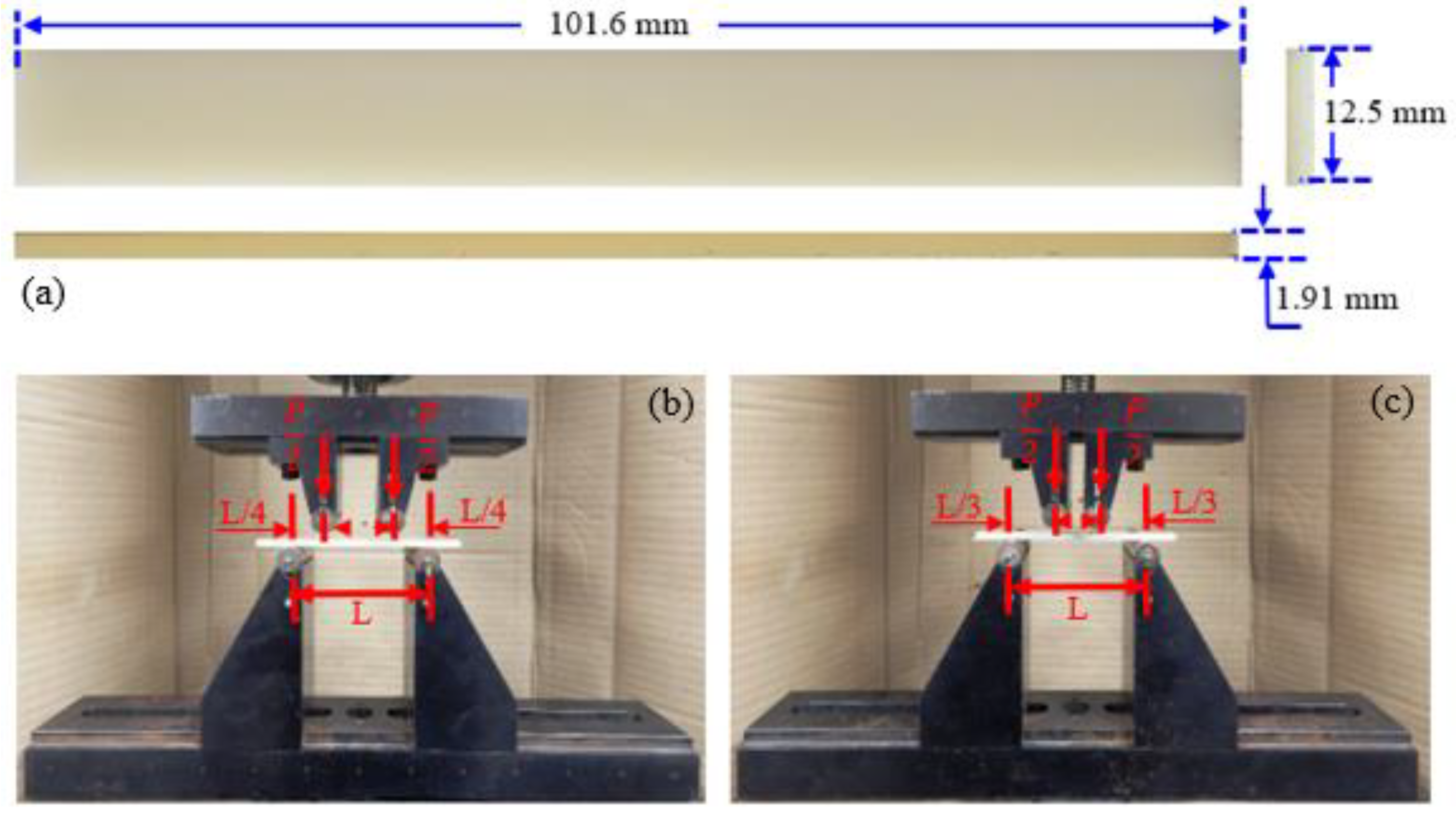
2. Materials and Methods

The four-point bending flexural test provides values for the modulus of elasticity in bending, flexural stress, flexural strain, and the flexural stress–strain response of the material. This test is very similar to the three-point bending flexural test. The major difference being that the addition of a fourth bearing brings a much larger portion of the beam to the maximum stress, as opposed to only the material right under the central bearing. The four-point bending is a conventional testing method that is analyzed by considering the shear and local deformation effects in the load application and supports. This test method is used widely for the determination of mechanical properties of materials especially subjected to bending force. The four-point bending test has also an advantage as a flexural test that sample geometries are easy to produce, and there are no gripping problems can occur in tensile tests. The raw materials of the polymer used was Cycolac EX58 ABS produced by Sabic ($\rho$: 1.03 g/cm³; Melting Temperature (T_m): 215–230 °C; MFR: 4 g/10min) and distributed by k-mac plastics. This raw material contains styrene, butadiene, and acrylonitrile monomers with a ratio of 65% to 70%, 20% to 25%, and 10% to 15%, respectively. The molecular weight of styrene, butadiene, and acrylonitrile monomers is 104.15 g/mol, 54.09 g/mol, and 53.03 g/mol, respectively. Standard specimens as stipulated for plastic materials were prepared according to ASTM D6272 guidelines. The geometric dimensions of the specimen are illustrated in Figure 1a. Flexural tests were carried out using a Material Testing System (MTS) machine with a load capacity of 22 kip. The experiments were conducted at room temperatures using a four-point bending fixture produced by Wyoming test fixtures Inc. The diameter of the supports and loading nose cylinders was 12.7 mm. Two types of load configurations were considered for conducting these four-point bending tests: short beams and long beams. The short beam load configuration applies compressive force to specimen at one quarter point loading with support span as 64 mm and load span as 32 mm. Similarly, the long beam configuration loads the specimen with one-third point loading having a support span of 64 mm and load span of 21 mm. Figure 1b,c show the test fixture and two specimen configurations during the four-point bending test. Quasi-static flexural tests were conducted in displacement control mode by pushing the bottom supports against the laminated beam at a rate of 3 mm/min.

Load, displacement, and time data were recorded for every 0.5 s by the computerized controlled machine. To obtain useful data, six samples of ABS (thickness 1.91 ± 0.04 mm) were tested, and the readings were averaged and combined into a single graph. The utilized material model of SAMP-1 in numerical implementations uses various experimental test data that can be obtained from tension, compression, shear, and biaxial tension tests. To define the strain rate-dependent material behavior, SAMP-1 requires the tension tests to be conducted at different deformation rates; therefore, we carried out tension tests on ABS at various deformation rates changing from 0.05 to 10 mm/s. Additionally, compression and shear tests were conducted on ABS under quasi-static conditions for identifying dissimilar material behavior in tension and in compression as well as shear. Uniaxial tension tests specimens of ABS were prepared depending on ASTM D638 Type I [25] standard, and the uniaxial tension tests were conducted at different deformation rates. To measure tensile strains, both the digital image correlation (DIC) optical method and extensometer were used during tensile tests. The tensile tests were conducted at four various deformation rates of 0.05 mm/s, 1 mm/s, 5 mm/s, and 10 mm/s resulting strain rates of 0.001 s⁻¹, 0.02 s⁻¹, 0.1 s⁻¹, and 0.2 s⁻¹, respectively. The plastic Poisson’s ratio distribution for the attained lowest strain rate of 0.001 s^-1 was calculated using true longitudinal strains and true transverse strains provided by DIC. The compression and shear test specimens were prepared based on ASTM D695-15 and ASTM D5379 standards, respectively. Although the ASTM D5379 is designed for the determination of shear properties of composite materials, this method is extensively utilized to define the shear properties of thermoplastics [26]. In reality, thermoplastics do not exhibit any shear fracture; therefore, shear fracture is not considered for the robust design of thermoplastics. During shear tests, DIC was set up to record shear strain distribution.

3. Numerical Modeling

As mentioned before, the material behavior of thermoplastics subjected to multiaxial loads such as four-point bending is highly sophisticated since their material behaviors are highly dominated by strain rate and pressure dependency. Therefore, selecting the best material model available in finite element codes to handle the complex material behavior of thermoplastics is highly crucial for accurate predictions. Hence, the particularly developed material model for polymers SAMP-1 in Ls-Dyna appears to be the best material model to cope with the complex material behavior of thermoplastics. Thus, SAMP-1 was selected as our constitutive material model in the numerical implementations of four-point bending tests. Nevertheless, SAMP-1 uses experimental test data as an input and it requires a significant number of mechanical tests. For instance, uniaxial tension tests over a wide range of strain rates to consider strain rate dependency and compression and shear tests to take pressure dependency into account. Therefore, at least three mechanical tests such as tension, compression, and shear need to be conducted, and measured values are supposed to be provided as an input to SAMP-1. With respect to introduced experimental data as an input to SAMP-1, there are three various yield surface definitions resulted by SAMP-1. The first one is the Von-Misses yield surface formulation that is achieved by utilizing only tension test data as an input in SAMP-1. Introducing only either shear test data with tension test data or compression test data with tension test data yields the Drucker–Prager yield surface definition. Providing tension, compression, and shear test data to SAMP-1 generates the actual yield surface definition of SAMP-1 known as the SAMP-1 yield surface. The short theoretical formulation of the SAMP-1 yield surface is provided here after referring to the LSDYNA Keyword [27] and Theory Manuals [28].

The yield surface of SAMP-1 can be expressed by the following formula:

$$f={\sigma }_{vm}^2-A_0-A_{1}p-A_2{p}^2\le 0$$

(1)

where $p$ is the first stress invariant and can be formulated as follows:

$$p=-\frac{{\sigma }_{xx}+{\sigma }_{yy}+{\sigma }_{zz}}{3}$$

(2)

and ${\sigma }_{vm}$ is the first stress invariant (Von Mises) and can be expressed as written below.

$${\sigma }_{vm}=\sqrt{\frac{3}{2}[{\left({\sigma }_{xx}+p\right)}^2+{\left({\sigma }_{yy}+p\right)}^2+{\left({\sigma }_{zz}+p\right)}^2+2{\sigma }_{xy}^2+2{\sigma }_{yz}^2+2{\sigma }_{xz}^2]}$$

(3)

The unknown constants of A₀, A₁, and A₂ can be extracted through using tension, compression, and shear test data as provided below:

$$A_0={\sigma }_s\sqrt{3}$$

(4)

$$A_1=3\left[\frac{{\sigma }_t-{\sigma }_C}{{\sigma }_t+{\sigma }_C}-{\sigma }_s\sqrt{3}\frac{{\sigma }_t-{\sigma }_C}{{\sigma }_t{\sigma }_C}\right]$$

(5)

$$A_2=18\left[\frac{1}{{\sigma }_t+{\sigma }_C}-\frac{{\sigma }_s\sqrt{3}}{2{\sigma }_t{\sigma }_C}\right].$$

(6)

In our four-point bending simulations, the response of ABS was predicted based on Von-Misses, Drucker–Prager, and SAMP-1 yield surfaces for the purpose of revealing the yield surface selection effect on predictions, and the predicted results were successfully compared to one another. There is a possibility to define two distinct flow rules named associated and non-associated in SAMP-1 depending upon the utilized plastic Poisson’s ratio definition. If the constant plastic Poisson’s ratio is used in simulation, the flow rule will be considered as associated flow. When the plastic Poisson’s ratio change with plastic strain is defined, it will generate the non-associated flow rule, which is the employed flow rule in the simulations. The flow rule expression can be given as written below:

$$\mathrm{g}=\sqrt{3{\mathrm{J}}_2+{\mathsf{\alpha }\mathrm{I}}_1}$$

(7)

where $\alpha$ is the plastic Poisson’s ratio distribution as a function of plastic strain, and $\alpha$ can be specified by the following expression:

$$\mathsf{\alpha }=\frac{1-2{\mathrm{v}}_{\mathrm{P}}}{2\left(1+{\mathrm{v}}_{\mathrm{p}}\right)}.$$

(8)

Even though the SAMP-1 material model has been developed for polymers in purpose, there are some restrictions encountered in the definition of the proper material behavior of polymers. For instance, this material model uses a constant elastic modulus regardless of strain rate; however, it is well known that the elastic modulus of polymers varies with strain rate. Moreover, compression and shear yield surfaces are increased with respect to the introduced multiple tensile stress–strain curves to SAMP-1; nevertheless, some polymers can be more sensitive to compression than tension. The finite element models of four-point bending tests are depicted in Figure 2, which include the long beam and short beam features. Both two supports and two indenters were modeled as a rigid body and while the real deformation rates achieved in the actual four-point bending tests were imposed to the indenters, the supports were completely fixed with boundary conditions. The contact regions of ABS four-point bending test specimen with the supports and indenters were divided into smaller elements for the objective of improving contact accuracy as well as overall accuracy. The contact forces were obtained through the automatic surface-to-surface contact described between supports, indenters, and the ABS specimen. To improve the contact for the spherical surfaces, the pinball algorithm was used with the automatic surface-to-surface contact. The reduced solid element formulation of ELFORM1 was used in the aim of reducing computational time.

3.1. The Utilized Test Data for ABS in SAMP-1

As stated previously, the SAMP-1 material model uses the tensile test data over a range of strain rates as well as quasi-static compression and quasi-static shear test data as an input. To be introduced to test data to SAMP-1, all the tests mentioned above were conducted, and the required test data for SAMP-1 was extracted. The tensile tests were conducted on ABS under various strain rates ranging from 0.001 s⁻¹ to 0.2 s⁻¹. The tensile strains were recorded utilizing DIC, which indicates the true tensile strain distribution on ABS shortly before it ruptures. The utilized tensile test data in simulations are illustrated in Figure 3a. In our simulations, the flow rule was considered as non-associated flow, implying that the plastic Poisson’s ratio as a function of plastic strain rather than constant plastic Poisson’s ratio was utilized as an input data in SAMP-1. The plastic Poisson’s ratio change with plastic strains was calculated using longitudinal and transverse strains that were measured by DIC during tensile tests. The used plastic Poisson’s ratio, compression, and shear test curves as input data in SAMP-1 are illustrated in Figure 3b. The SAMP-1 material model does not take elastic modulus change with strain rate into account. In other words, the SAMP-1 considers only one elastic modulus value given as an input. However, the tensile elastic modulus of ABS varies from strain rate to strain rate, as documented in

Table 1. Tensile elastic modulus of ABS with strain rates.

Strain Rate (1/s)	True Tensile Elastic Modulus (GPa)
0.001	1.826
0.02	1.938
0.1	2.026
0.2	2.070

. Therefore, the elastic modulus of ABS used in simulations was taken as 1.9735 GPa, which is the average value of the four elastic moduli tabulated in Table 1.

Table 2. The elastic material parameters of ABS used in simulations.

Bulk Modulus (GPa)	Tensile Modulus (GPa)	Poisson’s Ratio	Density (tonne/mm3)
3.59	1.9735	0.38	1024 × 10−12

displays the experimentally determined elastic material properties of ABS that were utilized in numerical analysis.

3.2. Damage Modeling

3.2.1. GISSMO Damage Model

GISSMO stands for generalized incremental stress-state dependent damage model [27]. The failure model formulation of GISSMO allows for an incremental description of damage accumulation, including softening and failure [27]. It provides an advantage of defining an arbitrary triaxiality dependent failure strain, which is required for the use over a wide range of different stress triaxialities and materials [28]. The damage variable is represented by an exponential function

$$\dot{D}=\frac{n}{{\epsilon }_f}{D}^{\left(1-\frac{1}{n}\right)}\dot{{\epsilon }_p}$$

(9)

where D is the current value of the damage, $\dot{{\epsilon }_p}$ is the equivalent plastic strain rate, n is the damage exponent, and ${\epsilon }_f$ is equivalent plastic strain at failure. The onset of necking is considered through the forming intensity parameter F.

$$\dot{F}=\frac{n}{{\epsilon }_{p,loc}}{F}^{\left(1-\frac{1}{n}\right)}\dot{{\epsilon }_p}$$

(10)

where ${\epsilon }_{p,loc}$ is the equivalent plastic strain to localization. Parameter F is also accumulated in the similar fashion as that of damage parameter D. The major difference between functions D and F lies in the type of the limiting strain depending on the triaxiality forms is used, ${\epsilon }_f$ or ${\epsilon }_{p,loc}$,. The damage in this formulation is coupled to the stress tensor using Lemaitre’s [29] effective stress concept, when the instability is reached, F = 1.

$${\sigma }_{eff}=\sigma \left(1-{\left(\frac{D-D_{crit}}{1-D_{crit}}\right)}^m\right)$$

(11)

The value for $D_{crit}$ is used as the indication for reaching the onset of necking. The exponent m is known as the fading exponent, which is utilized for a regularization of fracture strain and the energy consumed during post-instability deformation [27]. The GISSMO damage formulation was added to the SAMP-1 material law by using the *ADD_DAMAGE_GISSMO keyword card. The input curves used to model damage through GISSMO in this study are provided in Figure 4.

3.2.2. DIEM Damage Model

LSDYNA Theory and Keyword manual are referred to present the brief background on the damage formulation of Damage Initiation and Evolution (DIEM) [27,28]. In this damage formulation, an arbitrary number of damage initiation and evolution criteria can be defined and combined. The damage initiation and evolution history variables are assigned for each integration point in the case of multiple initiation/evolution types criteria are defined, ${\omega }_D^i\in \left[0,\infty \right] and D^i\in \left[0,1\right], i=1,\dots n$,.

The global damage $D\in \left[0,1\right]$ is formed by using the damage evolution variables which govern the damage in the material at each integration point. The global damage variable is defined as

$$D=max\left(D_{max},D_{mult}\right)$$

(12)

where

$$D_{max}=ma{x}_{\mathrm{i}\in I_{max}}{D}^i$$

(13)

$$D_{mult}=1-{П}_{\mathrm{i}\in I_{mult}}\left(1-D^i\right).$$

(14)

The functions ${\epsilon }_D^p={\epsilon }_D^p\left(\eta {\dot{\epsilon }}^p\right)$ and ${\epsilon }_D^p={\epsilon }_D^p\left(\theta {\dot{\epsilon }}^p\right)$ represent the plastic strain at the onset of the damage for the ductile and shear damage initiation options, respectively. The shear stress function is defined as

$$\theta =\left(q+k_{s}p\right)/\tau$$

(15)

where p is the pressure, q is the Von-Mises equivalent stress, and $\tau$ is the maximum shear stress defined as a function of principal stress values

$$\tau =\frac{\left({\sigma }_{major}-{\sigma }_{minor}\right)}{2}.$$

(16)

The damage initiation history variable in both cases evolves according to

$${\omega }_D={\int }_0^{{\epsilon }^p}\frac{d{\epsilon }^p}{{\epsilon }_D^p}.$$

(17)

The evolution of the associated damage variable D is governed through the introduction of the plastic displacement $u^p$. The evolution of plastic displacement is defined as

$${\dot{U}}_p=\{\begin{array}{r}0, {\omega }_D<1\\ h{\dot{\epsilon }}^p, {\omega }_D\ge 1\end{array}$$

(18)

where h is the characteristic length of the element used to suppress the mesh dependence. This quantity starts evolving after the corresponding damage initiation variable reaches unity and each criterion has its unique plastic displacement variable [27]. The damage variable evolves linearly with the plastic displacement in the linear damage evolution option.

$$\dot{D}=\frac{\frac{{\dot{U}}_p}{\partial U_f^p}}{\partial D}$$

(19)

where $U_f^p$ is the plastic displacement at the failure function. The plastic displacement at failure can be constant or depend on the triaxiality and damage i.e., $U_f^p=U_f^p\left(\eta ,D\right)$. The DIEM damage formulation was added to SAMP-1 material law by using the *ADD_DAMAGE_DIEM keyword card, and ductile damage initiation criteria based on stress triaxiality was chosen. The evolution of damage was governed by linear softening i.e., the evolution of damage is a function of the plastic displacement after the initiation of damage. Plastic displacement at failure was considered as 0.25 mm. Plastic strain at the onset of damage as function of stress triaxiality used for damage initiation is provided in Figure 5a.

3.2.3. Damage model of SAMP-1

The damage parameter d is a function of plastic strain only in the inherent damage model of SAMP-1 material law. This damage model is isotropic in nature and requires a load curve defining damage parameter d, as a function of true plastic strain under uniaxial tension. Critical damage leading to rupture is another input variable required by the model. Then, the implemented model uses the notion of an effective cross-section, which is the true cross-section of the material minus the cracks that have developed. Effective stress is defined as force divided by the effective cross-section.

$$\sigma =\frac{f}{A},{\sigma }_{eff}=\frac{f}{A_{eff}}=\frac{f}{A\left(1-d\right)}=\frac{\sigma }{\left(1-d\right)}$$

(20)

Therefore, effective yield stress is defined as:

$${\sigma }_{y,eff}=\frac{{\sigma }_y}{1-d}.$$

(21)

Using the strain equivalence principle, the effective stress corresponds to same elastic strain as the true stress using the damaged modulus if the undamaged modulus is used.

$$E=\frac{{\sigma }_{eff}}{{\epsilon }_e},E_d=\frac{\sigma }{{\epsilon }_e}=E\left(1-d\right)$$

(22)

As the plastic strain are same, therefore, it can be formulated as:

$${\epsilon }_p=\epsilon -\frac{{\sigma }_{e_{ff}}}{E}=\epsilon -\frac{\sigma }{E_d}.$$

(23)

Under pure elastic deformation, no damage will occur with this model. The damage parameter effectively reduces the elastic modulus. If unloading is performed at different strain values in the tensile test, the different unloading slopes allow estimating the damage parameter for a particular strain.

$$d\left({\epsilon }_{Pt}\right)=1-\frac{E_d\left({\epsilon }_{Pt}\right)}{E}$$

(24)

The input damage curve defined as function of true plastic strain used in this article is provided in Figure 5b.

3.2.4. Failure Modeling by EPFAIL and DEPRPT Parameters in SAMP-1 Material Law

The parameter EPFAIL is the Equivalent Plastic strain at FAILure. It can be defined as an absolute value or a load curve can be provided defining EPFAIL as a function of the plastic strain rate. The parameter DEPRPT is the increment of equivalent plastic strain between failure point and rupture point. The stresses will fade out to zero in the elements between EPFAIL and EPFAIL+DEPRPT points. The failure (erosion) of elements through EPFAIL and DEPRPT parameters was modeled in conjunction with the damage modeling, as explained in Section 3.2.1. EPFAIL and DERPT parameters were assumed as 0.12 and 0.02, respectively.

Several numerical simulations were performed with the long beam configuration correlated model having a loading rate of 0.5 mm/s to study the effect of an EPFAIL and DEPRPT parameters, GISSMO and DIEM damage models, strain rate effects, yield surfaces, and contact friction coefficient on the response predictions capabilities of SAMP-1 material law. The results of these simulations are illustrated in the next section of the article.

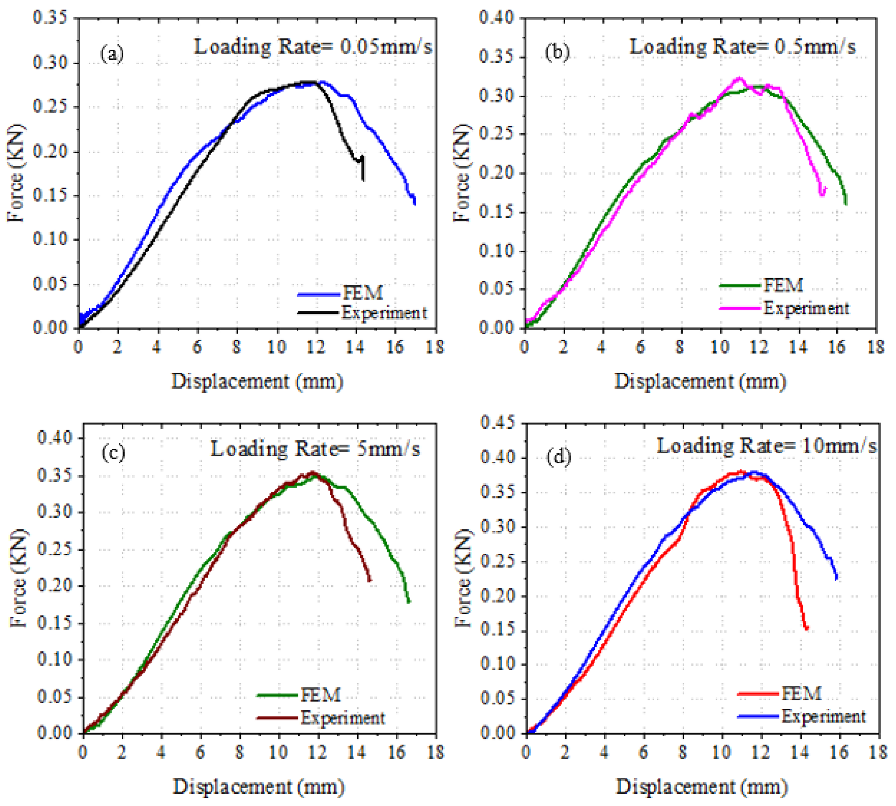
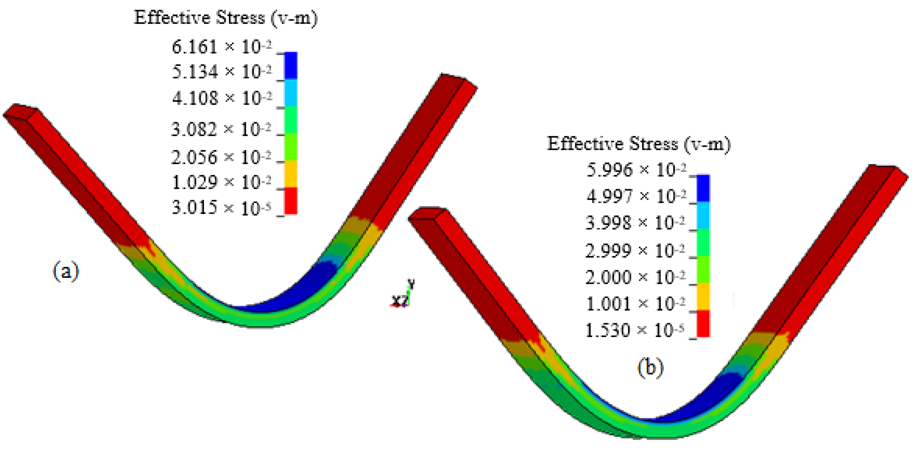
4. Results and Discussions

The experimental response of the ABS material under four-point loading conditions at different loading rates is compared for short-beam and long-beam configurations in Figure 6. Short-beam specimens require higher forces as compared to long-beam specimens at a particular loading rate. The response of the material changes under different loading rates for both categories of the specimens, but the material response under short-beam configuration is more susceptible to strain-rate effects than at higher loading rates.

The numerical predictions obtained through the MAT SAMP-1 model for ABS material being loaded at different loading rates in long span configuration are compared to the experimental results in Figure 7. The predicted volumetric strain contour of long-beam configuration at various deformation rates is illustrated in Figure 8. The volumetric strain increases from 0.064 to 0.127 with the increase in the loading rate from 0.05 to 10 mm/s in the long-span configuration, whereas it increases from 0.138 to 0.194 in the short-span beam configuration. A comparative analysis of numerical predictions and experimental findings for force displacement plots of short-span beams under different loading rates is presented in Figure 9. A discrepancy observed in the numerical predictions in the post-damage initiation stage is due to the fact that the damage model of the MAT SAMP-1 model was not activated in these simulations. The effect of considering the damage in the material model is studied as a sub-section in this article by taking an initial correlated model of a long-span beam having a loading rate of 0.5 mm/s. The contour plots of volumetric strain at a displacement of 16 mm under different loading rates for short-span beams are illustrated by Figure 10. It can be depicted from Figure 10 that as the span is reduced in the short-span beams, the occurrence of the volumetric strain is also localized near the vicinity of the load nose tips.

5. Parametric Simulations

This section of the article deals with the parametric simulations that were performed to study the effect of various calibration parameters of the MAT Samp-1 material model. A correlated model from a long-span beam configuration having a loading rate of 0.5 mm/s was used to perform these studies.

5.1. Yield Surfaces

Drucker–Prager, Von-Mises, and SAMP-1 yield surfaces can be considered in the formulation of a material model depending upon the definition of the stress–strain curves for tension, compression, shear, and/or biaxial tension. Von-Mises yield surfaces is obtained by inputting just one tensile stress–strain curve.

Drucker–Prager conical yield surface is achieved by inputting compression or shear stress–strain in addition to the tensile stress–strain curve. A comparative analysis of the load–displacement plots considering these yield surfaces in the MAT SAMP-1 material model is described in Figure 11a. A consideration of Von-Mises yield criteria results in lower force response as compared to the Drucker–Prager and SAMP-1 yield criteria. Figure 12 describes the comparison between these yield surfaces for the Von-Mises stress contours at the displacement of 16 mm. The level of Von-Mises stresses also increases as we change the yield surface from typical Von-Mises to the SAMP-1 yield surface.

5.2. Loading Rates

The behavior of ABS material was studied under four-point flexural loading by varying the displacement rates of loading nose as 0.25 mm/s and 0.5 mm/s and considering the SAMP-1 yield surface. For the material model to correctly predict the ABS response, tensile stress–strain curves at multiple strain rates were provided in the tabulated format to model, as shown in Figure 3a. The loading versus displacement plots for different loading rates are illustrated in Figure 11b. A slight increase in the peak load value of the predictions was observed as the rate of loading was increased from 0.25 to 0.5mm/s. The contour plots for Von-Mises stress with different loading rates at the displacement of 16 mm are shown in Figure 13.

5.3. Contact Friction

In order to study the effect of contact friction between supports and the load nose tip, there static (F_s) and dynamic (F_d) friction coefficients employed in automatic surface to surface contact were varied randomly in the ranges of F_s = 0.1–0.35 and F_d = 0.05–0.175. Figure 11c shows the force–displacement plots for the different iterations performed while studying the effect of contact friction considering the SAMP-1 yield surface. As expected, with the increase in the friction coefficients, it was found that the force required to bend the specimen also increases.

5.4. Damage Modeling

5.4.1. SAMP-1 Damage Formulation

A comparison between predictions resulted without accounting any damage formulation in the SAMP-1 material law (Baseline) and by activating the inherent damage formulation of SAMP-1 material is illustrated in Figure 14a. It can be observed that the inclusion of damage formulation in the material law results in the reduction of the peak force and also degrades the material response in the post-damage initiation phase of the force–displacement curve. Under pure elastic deformation, no damage had occurred with this damage model. The evolution of damage in the specimen at different simulation time steps is provided in Figure 15. The initiation of damage occurs at the displacement 5 mm with damage index being 5.3 × 10⁻³, and the damage index reaches about 0.23 at displacement 16.4 mm. The maximum damage index is 1.

5.4.2. GISSMO and DIEM Damage Formulation

Damage initiation and evolution was modeled through GISSMO and DIEM damage models as well. Comparative analysis of the force–displacement response considering these damage models is illustrated in Figure 14b. The evolution of the damage when using the GISSMO damage formulation is stored in an extra history variable #23, which needs to be activated through the *Database Extent Binary Keyword for the visual representation of damage. Figure 16 illustrates the damage evolution in specimen for GISSMO damage formulation. Similarly, the evolution of damage, when using the DIEM formulation, is stored in an extra history variable #27. Figure 17 illustrate the damage evolution in specimen for DIEM damage formulation.

The initiation of damage occurs approximately at similar displacement values in both GISSMO and DIEM damage formulation. The material failure through element deletion was triggered in the GISSMO damage formulation after reaching the displacement 14.7 mm; however, that was not the case in the DIEM formulation. It was observed that the initiation damage index (2.832 × 10⁻¹⁶) in the GISSMO formulation was smaller than that of the DIEM formulation damage index (1.032 × 10⁻²) at approximately the same displacements.

As expected, the inclusion of both damage formulations results in the degraded response of specimen after the damage initiation phase, which can also be clearly inferred from the force displacement plot shown in Figure 14b.

5.4.3. Material failure modeling with EPFAIL and DEPRPT parameters

In the next parametric study, the material failure in conjunction with the damage modeling was modeled through the EPFAIL and DEPRPT parameters of the SAMP-1 material law. The force–displacement plot showing the material failure through element deletion is compared to one without incorporating material failure through these parameters, which are shown in Figure 14c. The elements that reach the plastic strain value of 0.12 were designated as failed and were removed from the calculations, resulting in a sharp decrease in the force levels after reaching the displacement of 15.8 mm. The parameter DEPRPT is the increment of equivalent plastic strain between failure point and rupture point. It is used to fade out the stresses in the elements before the final rupture point and is employed to characterize the slope of the force–displacement curve in the post failure portion of plot. Finally, the comparative force–displacement plot showing the predictive response of material with all damage formulations, material failure, prediction without any damage, or material failure (baseline simulation) and experiment results is illustrated in Figure 14d. The inclusion of all damage formulation results in the degradation of material response in the post-damage initiation phase. Material failure was observed in the GISSMO damage formulation.

6. Conclusions

The flexural behavior of ABS thermoplastic under four-point bending is significantly affected by the span length and deformation rate. A color change from white to light white at the back surfaces of ABS specimens was observed for each deformation rate and span length, indicating that a craze formation happened in ABS during four-point bending tests. The color change is more noticeable in ABS with short span than long span, indicating that damage severity or craze formation is higher in ABS with short span. The four-point bending reaction forces for each deformation rate decreased more drastically in ABS with short span in comparison with long span after they reached their peak values; that is, the explanation of damage severity took place more in ABS with short span. It was noticed that the prediction accuracy in long span is higher compared to short span. It can be concluded that the SAMP-1 exhibits a difficulty predicting the flexural behavior of ABS in the elastic region, because it uses the constant tensile elastic modulus regardless of strain rate, but the tensile elastic modulus of ABS is highly influenced by the strain rate. Moreover, the compressive elastic modulus of ABS is higher than its tensile elastic modulus; therefore, the SAMP-1 material model requires some modifications to take the strain rate-dependent elastic modulus into account. In comparison with the SAMP-1 calculations, while the Von-Mises yield criteria predict the force much less, the Drucker–Prager yield surface formulation provides similar results. Nevertheless, the SAMP-1 and Drucker–Prager yield surface formulations were compared for the deformation rate of 0.5 mm/s, and the comparisons need to be made for higher deformation rates to reveal in a proper way whether or not they provide identical results.

References

1. Mulliken, A.D. Mechanics of Amorphous Polymers and Polymer Nanocomposites during High Rate Deformation; Massachusetts Institute of Technology: Cambridge, MA, USA, 2006. [Google Scholar]
2. Rösler, J.; Harders, H.; Bäker, M. Mechanical Behaviour of Engineering Materials: Metals, Ceramics, Polymers, and Composites; Springer Science & Business Media: Berlin/Heidelberg, Germany, 2007. [Google Scholar]
3. Dean, G.; Wright, L. An evaluation of the use of finite element analysis for predicting the deformation of plastics under impact loading. Polym. Test. 2003, 22, 625–631. [Google Scholar] [CrossRef]
4. Altenbach, H.; Tushtev, K. A new static failure criterion for isotropic polymers. Mech. Compos. Mater. 2001, 37, 475–482. [Google Scholar] [CrossRef]
5. Galeski, A. Strength and toughness of crystalline polymer systems. Prog. Polym. Sci. 2003, 28, 1643–1699. [Google Scholar] [CrossRef]
6. Rabinowitz, S.; Ward, I.; Parry, J. The effect of hydrostatic pressure on the shear yield behaviour of polymers. J. Mater. Sci. 1970, 5, 29–39. [Google Scholar] [CrossRef]
7. Ognedal, A.S. Large-Deformation Behaviour of Thermoplastics at Various Stress States: An Experimental and Numerical Study. Ph.D. Thesis, Norwegian University of Science and Technology, Trondheim, Norway, 2012. [Google Scholar]
8. Qi, H.; Boyce, M. Stress–strain behavior of thermoplastic polyurethanes. Mech. Mater. 2005, 37, 817–839. [Google Scholar] [CrossRef]
9. Boyce, M.C.; Parks, D.M.; Argon, A.S. Large inelastic deformation of glassy polymers. part I: Rate dependent constitutive model. Mech. Mater. 1988, 7, 15–33. [Google Scholar] [CrossRef]
10. Argon, A.S. A theory for the low-temperature plastic deformation of glassy polymers. Philos. Mag. A J. Theor. Exp. Appl. Phys. 1973, 28, 839–865. [Google Scholar] [CrossRef]
11. Eyring, H. Viscosity, Plasticity, and Diffusion as Examples of Absolute Reaction Rates. J. Chem. Phys. 1936, 4, 283–291. [Google Scholar] [CrossRef]
12. Spathis, G. Theory for the plastic deformation of glassy polymers. J. Mater. Sci. 1997, 32, 1943–1950. [Google Scholar] [CrossRef]
13. Roetling, J.A. Yield stress behaviour of polymethylmethacrylate. Polymer 1965, 6, 311–317. [Google Scholar] [CrossRef]
14. Bauwens, J.C.; Bauwens-Crowet, C.; Homès, G. Tensile yield-stress behavior of poly(vinyl chloride) and polycarbonate in the glass transition region. J. Polym. Sci. Part A-2 Polym. Phys. 1969, 7, 1745–1754. [Google Scholar] [CrossRef]
15. Bowden, P.B.; Raha, S. A molecular model for yield and flow in amorphous glassy polymers making use of a dislocation analogue. Philos. Mag. 1974, 29, 149–166. [Google Scholar] [CrossRef]
16. Arruda, E.M.; Boyce, M.C. Evolution of plastic anisotropy in amorphous polymers during finite straining. Int. J. Plast. 1993, 9, 697–720. [Google Scholar] [CrossRef]
17. Raghava, R.; Caddell, R.M.; Yeh, G.S. The macroscopic yield behaviour of polymers. J. Mater. Sci. 1973, 8, 225–232. [Google Scholar] [CrossRef] [Green Version]
18. Caddell, R.M.; Raghava, R.S.; Atkins, A.G. Pressure dependent yield criteria for polymers. Mater. Sci. Eng. 1974, 13, 113–120. [Google Scholar] [CrossRef] [Green Version]
19. Whitney, W.; Andrews, R.D. Yielding of glassy polymers: Volume effects. J. Polym. Sci. Part C: Polym. Symp. 1967, 16, 2981–2990. [Google Scholar] [CrossRef]
20. Mulliken, A.; Boyce, M. Mechanics of the rate-dependent elastic–plastic deformation of glassy polymers from low to high strain rates. Int. J. Solids Struct. 2006, 43, 1331–1356. [Google Scholar] [CrossRef] [Green Version]
21. Bowden, P.; Jukes, J. The plastic flow of isotropic polymers. J. Mater. Sci. 1972, 7, 52–63. [Google Scholar] [CrossRef]
22. Ratai, A.; Kolling, S.; Haufe, A.; Feucht, M.; Bois, P.D. Validation and Verification of Plastics under Multiaxial Loading. In Proceedings of the 7th GERMAN LS-DYNA Forum, Bamberg, Germany, 30 September 2008. [Google Scholar]
23. Kolling, S.; Haufe, A.; Feucht, M.; Bois, P.D. A Constitutive Formulation for Polymers Subjected to High Strain Rates. In Proceedings of the 9th International LS-DYNA User Conference, Dearborn, MI, USA, 1–6 June 2008. [Google Scholar]
24. Vitali, M.N.-M. Characterization of Polyolefins for Design under Impact: From True Stress/Local Strain Measurements to the FE Simulation with LS-Dyna Mat. SAMP-1. In Proceedings of 7th German LSDYNA Forum, Bamberg, Germany, 30 September 2008. [Google Scholar]
25. Daiyan, H.; Andreassen, E.; Grytten, F.; Osnes, H.; Gaarder, R.H. Shear testing of polypropylene materials analysed by digital image correlation and numerical simulations. Exp. Mech. 2012, 52, 1355–1369. [Google Scholar] [CrossRef]
26. Standard, A.S.T.M. Standard Test Method for Tensile Properties of Plastics; ASTM International: Designation: West Conshohocken, PA, USA, 2014; Volume D638, pp. 1–14. [Google Scholar]
27. Livermore Software Technology Corporation (LSTC). Livermore Software Technology Corporation, LS DYNA Version 971, Keyword User’s Manual; Livermore Software Technology Corporation (LSTC): Livermore, CA, USA, 2017; Volume II Material Models. [Google Scholar]
28. Livermore Software Technology Corporation (LSTC). Livermore Software Technology Corporation, LS DYNA Version 971, Theory Manual; Livermore Software Technology Corporation (LSTC): Livermore, CA, USA, 2017. [Google Scholar]
29. Lemaitre, J. A Continuous Damage Mechanics Model for Ductile Fracture. J. Eng. Mater. Technol. 1985, 107, 83–89. [Google Scholar] [CrossRef]
Figure 1. (a) Geometric dimensions of the four-point bending test specimen; (b,c) four-point flexural test setup pertaining to two span lengths.
Jcs 04 00063 g001
Figure 2. Finite element models for four-point bending cases. (a) Short beams, (b) long beams.
Jcs 04 00063 g002
Figure 3. Input data for Acrylonitrile–Butadiene–Styrene (ABS) in Semi-Analytical material model (SAMP-1); (a) Tensile test, (b) compression, shear, and plastic Poisson’s ratio data.
Jcs 04 00063 g003
Figure 4. Input curves utilized for the Generalized Incremental Stress-State MOdel (GISSMO) damage Model.
Jcs 04 00063 g004
Figure 5. (a) Plastic strain at the onset of damage as function of stress triaxiality; (b) Damage parameter, d vs. true plastic strain.
Jcs 04 00063 g005
Figure 6. Comparison for the behavior of short and long-span beams under four-point flexural loading.
Jcs 04 00063 g006
Figure 7. Comparison between experimental and FEM predictions for the behavior of long-span beams.
Jcs 04 00063 g007
Figure 8. Contour plots of long-beam configuration for volumetric strain at different loading rates (a) 0.05 mm/s, (b) 0.5 mm/s, (c) 5 mm/s, and (d) 10 mm/s.
Jcs 04 00063 g008
Figure 9. Comparison between experimental and FEM predictions for the behavior of short-span beams.
Jcs 04 00063 g009
Figure 10. Contour plots of short beam configuration for volumetric strain at different loading rates (a) 0.05 mm/s, (b) 0.5 mm/s, (c) 5 mm/s, and (d) 10 mm/s.
Jcs 04 00063 g010
Figure 11. (a) Comparative analysis of load–displacement plots considering different yield surfaces in a MAT SAMP-1 material model (deformation rate: 0.5 mm/s); (b) Comparison of force–displacement response at different loading rates; (c) Effect of static and dynamic contact friction coefficient on the flexural response of short-span beams.
Jcs 04 00063 g011
Figure 12. Von-Mises stress contour plots, (a) Von-Mises, (b) Drucker–Prager, and (c) SAMP-1 yield surfaces (deformation rate: 0.5 mm/s).
Jcs 04 00063 g012
Figure 13. Von-Mises contour plots at two different loading rates, (a) 0.25 mm/s and (b) 0.5 mm/s.
Jcs 04 00063 g013
Figure 14. Comparison of force–displacement plots with different damage modeling formulations.
Jcs 04 00063 g014
Figure 15. Evolution of damage with the inherent damage law of SAMP-1 material model at different indenter displacements: (a) 5 mm, (b) 7 mm (c) 8.8 mm, (d) 11.2 mm, (e) 14 mm, and (f) 16.4 mm.
Jcs 04 00063 g015
Figure 16. Evolution of damage with the addition of GISSMO damage formulation to SAMP-1 material law at different indenter displacements: (a) 5 mm, (b) 8.8 mm, (c) 11.2 mm, and (d) 14 mm.
Jcs 04 00063 g016
Figure 17. Evolution of damage with the addition of DIEM damage formulation to SAMP-1 material law at different indenter displacements: (a) 7.7 mm, (b) 10 mm, (c) 13.8 mm, and (d) 16.7 mm.
Jcs 04 00063 g017