Non-Isothermal Process of Liquid Transfer Molding: Transient 3D Simulations of Fluid Flow Through a Porous Preform Including a Sink Term

Abstract

Resin Transfer Molding (RTM) is a widely used composite manufacturing process where liquid resin is injected into a closed mold filled with a fibrous preform. By applying this process, large pieces with complex shapes can be produced on an industrial scale, presenting excellent properties and quality. A true physical phenomenon occurring in the RTM process, especially when using vegetable fibers, is related to the absorption of resin by the fiber during the infiltration process. The real effect is related to the slowdown in the advance of the fluid flow front, increasing the mold filling time. This phenomenon is little explored in the literature, especially for non-isothermal conditions. In this sense, this paper does a numerical study of the liquid injection process in a closed and heated mold. The proposed mathematical modeling considers the radial, three-dimensional, and transient flow, variable injection pressure, and fluid viscosity, including the effect of liquid fluid absorption by the reinforcement (fiber). Simulations were carried out using Computational Fluid Dynamic tools. The numerical results of the filling time were compared with experimental results, and a good approximation was obtained. Further, the pressure, temperature, velocity, and volumetric fraction fields, as well as the transient history of the fluid front position and injection fluid volumetric flow rate, are presented and analyzed.

1. Introduction

Nowadays, society’s technological demands require the use of materials with unusual combinations of properties, which generally cannot be met by ceramic materials, metals, or polymers alone. However, they are fully satisfied by the use of composite materials, which have been well used in a wide variety of applications, such as in the defense, aerospace, automotive, sports, medical, and consumer industries, among others [1]. In the aerospace industry, the following applications can be mentioned: satellites, space centers, launch vehicles, spaceports, remote manipulator arms, and cargo bay doors, among others. In the automotive industry, the following applications can be mentioned: body and door panels, engine blocks, drive shafts, automotive brakes, clutch discs, bumpers, frames, and rocker covers, among others.

This situation is easily proven when one observes, in recent decades, the growing application of composites to replace traditional materials, especially in the aerospace industry [2]. It should be noted that the composites market in 2022 was estimated at USD 106 billion and is projected to have a compound annual growth rate of 6.1%, reaching USD 191 billion in 2032 [3], proving the great current and future importance of this segment.

Among the different manufacturing processes of polymeric matrix composites, liquid molding in closed molds can be mentioned, which has relevant industrial importance as it enables large-scale production with less environmental impact when compared to other production processes [4]. In the list of processes for the production of composites by liquid molding, there is Resin Transfer Molding, well known as RTM. This technique consists of the injection of a low-viscosity thermoset resin into a closed mold containing a dry fibrous preform [5].

The production of polymer matrix composites by RTM has been widely used because it has several advantages over other production processes [6,7]. The following are some of them: easy daily operation; reduced labor costs; reduced production time; parts produced with good surface quality; the possibility of manufacturing large parts; a wide range of usable reinforcements; applicability for production of parts of complex geometries; the final product has good dimensional tolerances; low material wastage; low environmental impact; flexibility of the tools used in the process; the possibility of adding inserts to the product; low exposure of operators to the chemicals used in the process; the low possibility of an air presence inside the product; and the low cost, eliminating the use of complex and expensive equipment such as compression rollers.

Among the factors that affect the RTM composite production process are the resin properties, mold geometry, fiber–resin interaction, fiber volumetric fraction, injection pressure, resin injection points in the mold, air outlet points in the mold, and mold temperature [8,9], and it is necessary to control all these parameters to obtain composites with high quality, aiming at minimizing production costs and increasing the quality of the product obtained post-process.

Due to the thermal dynamics of the RTM process, the viscosity of the resin varies as the injection into the mold progresses, which is a critical point of production control. The flow of the high viscosity resin inside the porous medium is more difficult, causing partial infiltration in some regions of the mold and increasing the void fraction, which is responsible for the reduction in the mechanical properties of the composite material.

In order to optimize the flow of resin inside the porous medium, it is possible to use heated molds, which causes a reduction in the viscosity of the resin, facilitates its impregnation in the reinforcement and, consequently, reduces the total time of filling the mold [10].

On the other hand, the absorption of resin by the fibrous reinforcement, that is, the infiltration of the resin into the micropores between the individual fibers of the fiber bundles, is a relevant physical phenomenon present in the production process by RTM [8]. The complete understanding and modeling of this absorption phenomenon is fundamental for the improvement of the RTM process, also contributing to the minimization of the fraction of voids in the composite produced, being of interest to the academic and industrial environment, especially with regard to composites produced with high quality standards, essential, for example, in aeronautical and aerospace applications [11,12].

In the experimental context, studies related to the RTM process can be easily found in the literature [13,14,15,16,17,18,19]; however, there is little research that evidences the phenomenon of resin retention by reinforcement [20,21].

On the other hand, when analyzing the current panorama of studies related to mathematical models and computer simulation applied to the production process of composites by RTM, it is verified that there is a large number of studies that make use of simplified modeling. These models often consider the isothermal and single-phase flow (resin only), disregarding the effect of the presence of air in the mold and considering the viscosity of the resin constant [22,23,24,25]. These considerations approximate the numerical results of simplified analytical models.

Another group of works, which are less numerous, insert the physical effect of multiphase flow (resin–air) in their mathematical models, bringing numerical simulations closer to the real physical phenomenon, but still considering the viscosity of the resin constant [26,27,28]. The consideration of the multiphase flow allows the evaluation of the air–resin interaction, making it possible, for example, to evaluate possible points of air trapping in the produced composite. It is, therefore, a more careful and complex analysis.

A small number of studies insert another complicating factor in the modeling, in addition to multiphase flow, which would be the consideration of non-isothermal flow [29]. The effect of inserting the energy conservation equation in the mathematical model allows the evaluation of a new range of production parameters, such as the resin temperature during the infiltration process and the mold temperature, thus allowing the optimization of production processes and better understanding of the evolution of the resin curing process and the effect of temperature gradients in the resin–air–porous medium thermo-fluid dynamic system on the quality of the composite produced.

There is also intermediate modeling, where single-phase non-isothermal flow is considered, with the viscosity of the resin variable [30,31,32,33] or constant [34,35]. This type of model allows the evaluation of the thermal effect in the process, without inserting in the modeling the physical and numerical complications of the multiphase flow; however, this provides a lower degree of detail of the process.

Finally, it is also verified that there is initial research into the macroscopic approach, with simplified models (isothermal and monophase flow, with constants including the fluid properties and injection pressure) examining the effect of resin absorption by the micropores of the reinforcing fibers [8,9,36]. The infiltration of the resin by the fiber reduces the depth of penetration and delays pressure stabilization, which generates the need to optimize the interactions between the fiber and resin inside the closed mold. However, despite the importance of this research, it is necessary to apply the consideration of the effect of resin absorption by the fiber in more elaborate and robust models, especially using powerful CFD tools, in order to increase and deepen the degree of understanding of the RTM process. For a better understanding of the importance of the sink term, its effect on the RTM process should be indicated to depend on the fiber architecture: for example, if the resin flow occurs along the fiber-to-fiber direction, the resin flows easily through the channels between fibers instead of impregnating the fibers completely; on the other hand, when the resin flow is perpendicular to the fiber directions, the resin tends to flow more evenly with a lower delayed effect, influenced to a lesser extent by the pressure drop at the inlet.

In view of the above, it is evident that there is a lack of a more robust and complete numerical model in the literature to describe the RTM process, especially with regard to resin absorption by the fibrous reinforcement in radial infiltration processes. In this sense, the present research aims to contribute to the numerical study (via CFD) of the composite manufacturing process by RTM, filling this gap. The proposed three-dimensional and non-isothermal multiphase mathematical modeling considers the transient flow regime, variable viscosity of the injected fluid, and variable injection pressure, and includes the phenomenon of absorption of the injected fluid by the micropores of the fibrous reinforcement. Thus, this work intends to help researchers and engineers with better understanding and modeling the physical phenomena that govern the manufacturing process of composites by RTM, especially in radial systems.

2. Methodology

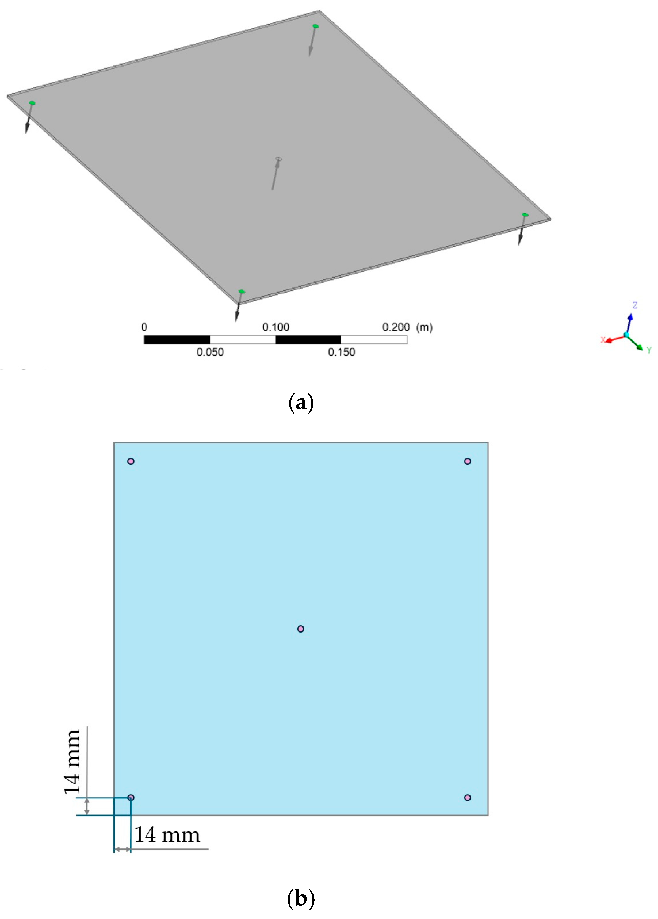
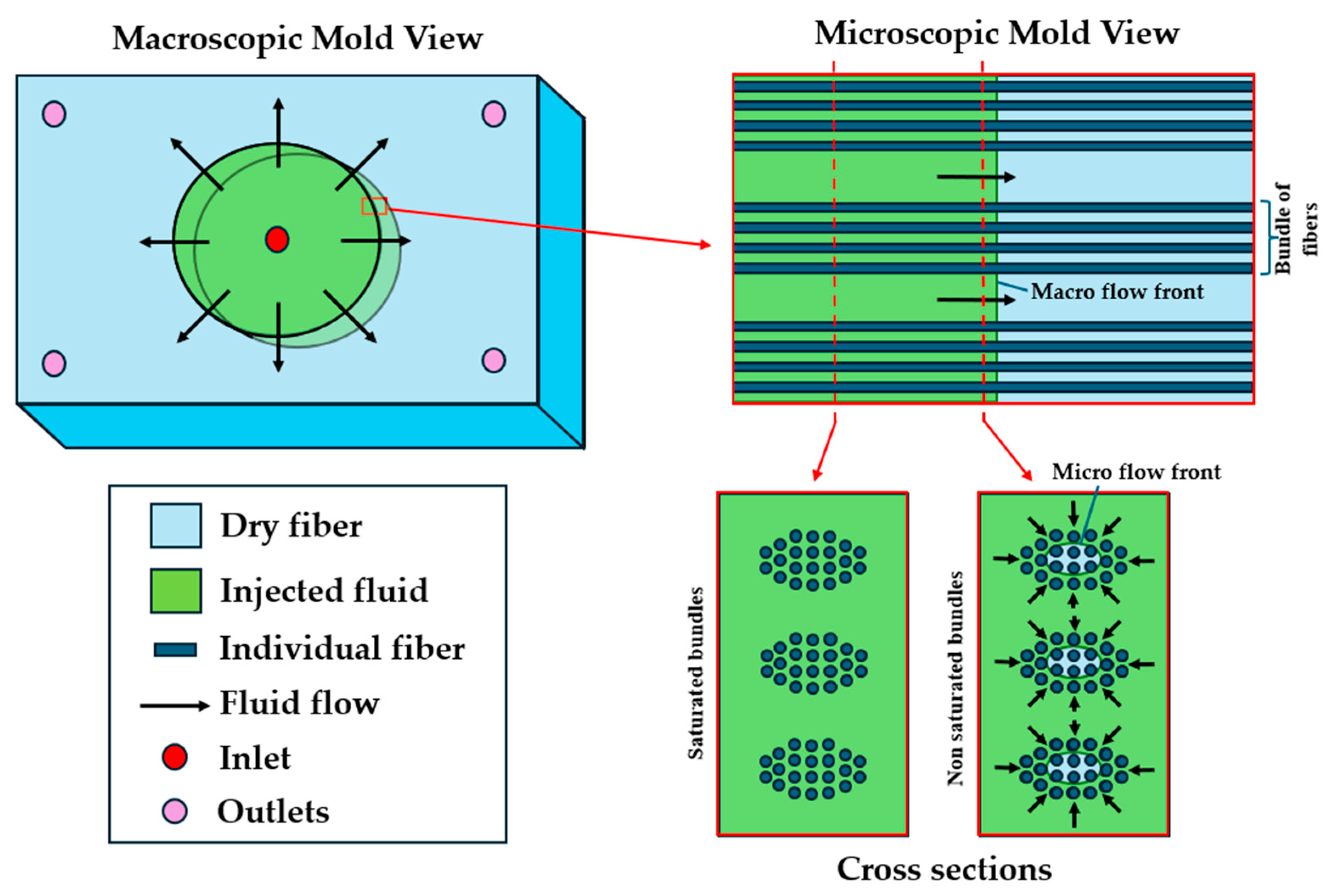
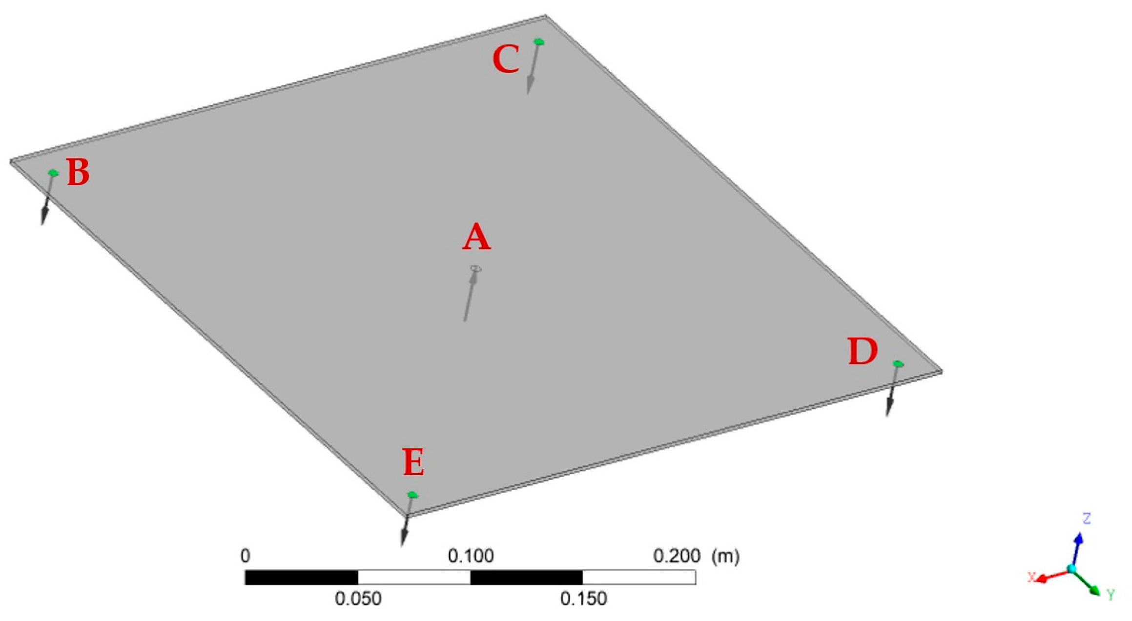
2.1. The Physical Problem and Mold Geometry

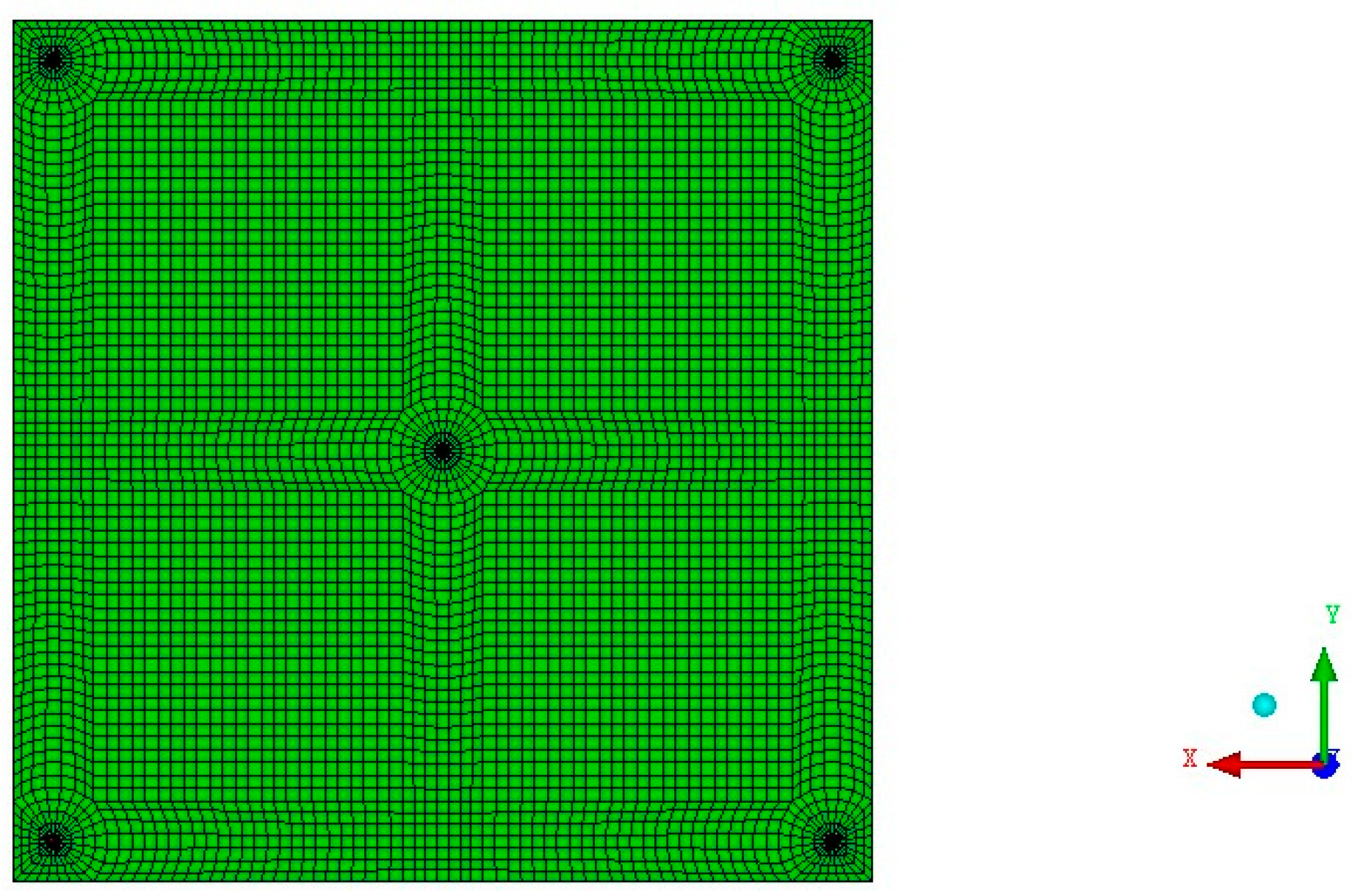
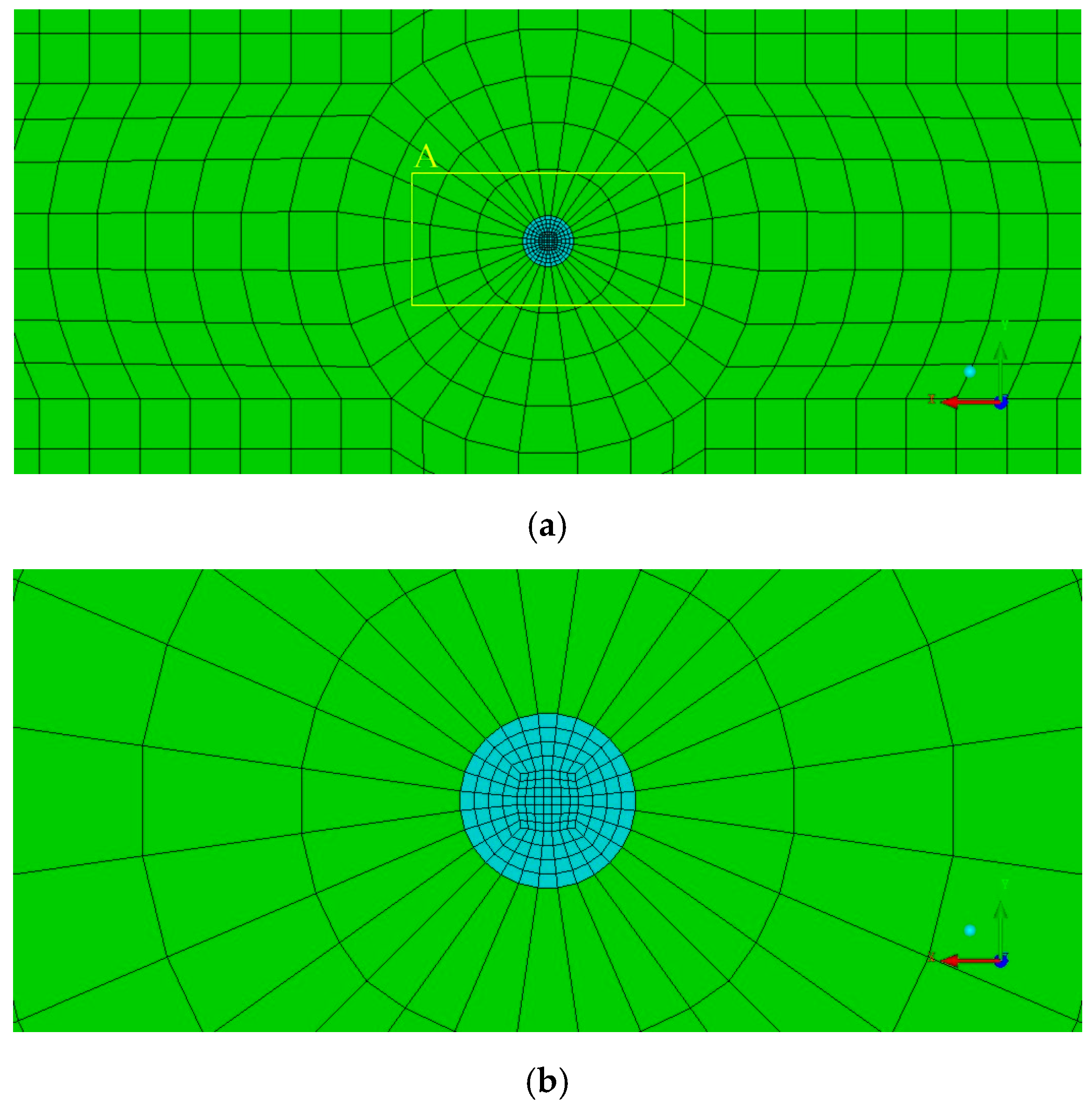
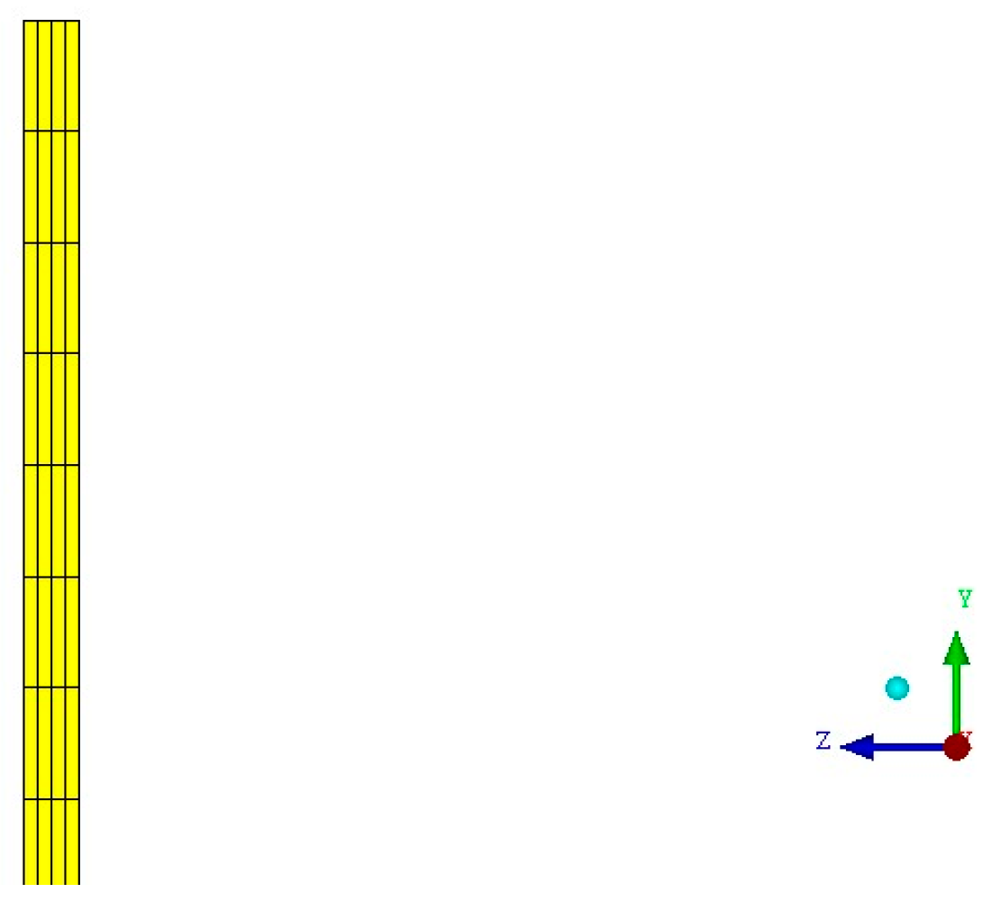
In this research, the fluid flow in a porous medium contained in a closed and heated mold is theoretically studied. The fluid is injected at the center of the mold and flows radially towards the exit gates located at the corners of the mold, exchanging heat with the reinforcement and with the mold walls.

The analyzed mold is parallelepipedal with a square base, with an area of 300 × 300 mm², thickness of 2 mm, and an injection point located in the center of the mold, as well as four symmetrical exit points positioned next to its vertices, as illustrated in Figure 1. All injection and exit points are radial holes with a diameter of 4.58 mm and are positioned at the bottom of the mold, i.e., the injection is ascending and the outlets are descending.

2.2. Numerical Mesh

To study the impact of mesh refinement on the numerical results, the Global Convergence Index (GCI) method was used. The GCI method has been used by several researchers [37,38] and estimates the discretization errors related to the degree of refinement of the numerical mesh used [39]. At the end of this stage, an optimized numerical mesh was obtained, which was structured and composed of 22,852 hexahedral elements, with 29,260 nodes, as illustrated in Figure 2, Figure 3, Figure 4 and Figure 5. This numerical mesh was built using the Ansys Icem CFD 2021 R2 trading software, and the simulations were run using the Ansys CFX 2021 R2 trading software. Ansys CFX was used instead of software dedicated to the RTM process, such as PAM-RTM, because it has a wider range of numerical models available, including for multiphase flow and heat transfer, in addition to allowing modification and implementation of the differential equations that physically govern the phenomena.

2.3. Mathematical Modeling

2.3.1. The Conservation Equations

To investigate the multiphase flow of injected fluid and air inside a heated mold, filled with fibrous reinforcement (porous medium), during the composite manufacturing process by RTM, the following considerations were adopted in mathematical modeling:

(a)

Three-dimensional, transient, non-isothermal, and laminar flow;

(b)

Incompressible fluid;

(c)

Isotropic porous medium;

(d)

No internal heat generation;

(e)

The injection pressure and viscosity of the injected fluid are variables;

(f)

The phenomenon of absorption of the injected fluid by the fibrous reinforcement is considered.

Figure 6 illustrates the phenomenon of fluid infiltration into the micropores inside the bundles of reinforcing fiber yarns.

To predict the behavior of the fluid inside the porous medium during the infiltration process, the general equations of the conservation of mass, momentum, and energy were used, considering a homogeneous multiphase model, i.e., a single velocity field for both fluids. These basic equations are shown in sequence:

(a)

Mass conservation equation:

The general equation of mass conservation for the fluid injected into the mold is as follows:

$${\displaystyle \frac{\partial }{\partial t}}\left(f_r\phi {\rho }_r\right)+\nabla ·\left({f_r\rho }_r{\overrightarrow{U}}_m\right)=-S^M=-s{\rho }_r$$

(1)

where φ represents the porosity of the porous medium (ratio between the volume of voids and the total volume of the porous medium); f_r is the volumetric fraction of the injected fluid; ρ_r is the density of the injected fluid; U_m is the surface velocity vector of the fluids; S^M is the source term that represents the mass flow rate of fluid injected, per unit volume of that fluid absorbed by the porous medium; and s is the source term that represents the mass flow rate of fluid injected, per unit mass of that fluid absorbed by the porous medium.

The general equation of mass conservation applied for the fluid (air) inside the mold is of the following form:

$${\displaystyle \frac{\partial }{\partial t}}\left(f_a\phi {\rho }_a\right)+\nabla ·\left({f_a\rho }_a{\overrightarrow{U}}_m\right)=0$$

(2)

where f_a is the volumetric fraction of the air, and ρ_a is the density of the air.

The volumetric fractions of the injected fluid and the air, at any point in the porous medium, are related as follows:

$$f_r+f_a=1$$

(3)

(b)

Linear Momentum Conservation Equation:

The conservation equation of the linear momentum is of the following form:

$${\displaystyle \frac{\partial }{\partial t}}\left(\phi {\rho }_m{\overrightarrow{U}}_m\right)+\nabla ·\left({\rho }_m{\overrightarrow{U}}_m\otimes {\overrightarrow{U}}_m\right)-\nabla ·\left[{\mu }_m\left(\nabla {\overrightarrow{U}}_m+{\left(\nabla {\overrightarrow{U}}_m\right)}^T-{\displaystyle \frac{2}{3}}\delta \nabla ·{\overrightarrow{U}}_m\right)\right]=\phi \overrightarrow{S^{\alpha }}-\phi \nabla p$$

(4)

where ρ_m is the weighted density of the fluids, µ_m is the weighted dynamic viscosity of fluids, δ is the unitary vector, S^α is the source term of linear momentum, and p is the pressure, including the gravitational effect.

The weighted density of the fluids is calculated as follows:

$${\rho }_m={f_r\rho }_r+{f_a\rho }_a$$

(5)

The weighted dynamic viscosity of the fluids is calculated as follows:

$${\mu }_m={f_r\mu }_r+{f_a\mu }_a$$

(6)

where µ_r is the dynamic viscosity of the injected fluid and µ_a is the dynamic viscosity of the air.

The source term of linear momentum, S^α, includes in modeling a loss of motion due to the yield strength caused by the porous medium, given as follows:

$$\overrightarrow{S^{\alpha }}=-{\displaystyle \frac{{\mu }_m}{K}}{\overrightarrow{U}}_m-K_{loss}{\displaystyle \frac{{\rho }_m}{2}}\left|{\overrightarrow{U}}_m\right|{\overrightarrow{U}}_m$$

(7)

where K_loss is the quadratic moment loss coefficient and K is the permeability of the porous medium. In this research, the second term was considered null, due to the low velocities to which the studied flow is subjected.

(c)

Energy Conservation Equation:

To include the thermal effect in the simulations, it is necessary to add the energy balance to the system of conservation equations. In this equation, a non-homogeneous multiphase flow was considered, i.e., distinct temperature fields for each of the fluid phases and for the solid (porous medium). In this case, the energy conservation equation is as follows:

• For the injected fluid, it was calculated as follows:

$${\displaystyle \frac{\partial }{\partial t}}\left({f_r\phi \rho }_r{h}_r\right)+\nabla ·\left({f_r\rho }_r{\overrightarrow{U}}_m{h}_r\right)-\nabla ·\left({f_{r}k}_r\nabla T_r\right)=0$$

(8)

where h_r is the enthalpy per mass unit of the injected fluid, k_r is the thermal conductivity of the injected fluid, and T_r is the temperature of the injected fluid.

• For the air, it was calculated as follows:

$${\displaystyle \frac{\partial }{\partial t}}\left({f_a\phi \rho }_a{h}_a\right)+\nabla ·\left({f_a\rho }_a{\overrightarrow{U}}_m{h}_a\right)-\nabla ·\left({f_{a}k}_a\nabla T_a\right)=0$$

(9)

where h_a is the enthalpy per unit mass of the air, k_a is the thermal conductivity of the air, and T_a is the temperature of the air inside the mold.

• For the porous medium (fibrous preform), it was calculated as follows:

$${\displaystyle \frac{\partial }{\partial t}}\left[{\left(1-\phi \right)\rho }_s{C_{s}T}_s\right]-\nabla ·\left(k_s\nabla T_s\right)=0$$

(10)

where ρ_s is the density of the porous medium, C_s is the specific heat of the porous medium, k_s is the thermal conductivity of the porous medium, and Ts is the temperature of the porous medium.

The Reynolds number is a relevant dimensionless parameter for characterizing a flow, representing the ratio between the inertial forces and viscous forces acting on the fluid. For a fluid flowing into a porous medium, this dimensionless parameter can be expressed as follows [40]:

$${Re}_{pm}={\displaystyle \frac{{\rho }_r\times U\times \sqrt{K}}{{\mu }_r}}$$

(11)

where Re_pm is the Reynolds number for flow in porous media and U is the surface velocity of the fluid in the direction of flow.

It should be noted that it is not necessary to add equations that govern the phenomenon of turbulence to the proposed mathematical model, since the Reynolds number for flow in porous media calculated by Equation (11), for this research, is approximately 2 × 10⁻⁵, and is therefore much lower than 1, so that the flow is classified as laminar in the Darcy regime.

2.3.2. Boundary Conditions

Figure 7 illustrates the study domain (mold) with emphasis on the injection point (A) and the four exit points (B–E). The boundary conditions to which the domain is subject are as follows:

(a)

Injection channel (point A):

The injection of vegetable oil, with a temperature of 23 °C and prescribed gauge pressure as a function of time, can be modeled as follows [41]:

$$p_{inj}=\left\{\begin{array}{c}305.6180\times t , for t<89 s\\ \mathrm{27,200} , for t\ge 89 s\end{array}\right.$$

(12)

where p_inj is the injection gauge pressure (Pa) and t is the time (s).

(b)

Output channels (points B–E):

The prescribed gauge pressure is null.

(c)

Mold walls:

The fluid velocity is zero (non-slip hypothesis), with a prescribed temperature of 60 °C.

(d)

Porous medium:

The prescribed initial temperature is equal to 60 °C, and the medium is fully filled with initially static air (zero velocity), with a prescribed initial temperature equal to that of the porous medium (60 °C).

2.4. Properties of Materials

The porous medium studied is a commercial flat fabric 0/90° type E fiberglass (300 g/m²), with the properties described in Table 1. For s = 0 s⁻¹, the permeability of this porous medium was calculated using Equation (13) [8]. For s = 0.5 × 10⁻⁴ s⁻¹, the permeability was estimated based on the experimental results [41].

$$K={\displaystyle \frac{{\mu }^{*}\times \phi }{2{\int }_0^{t_{ff}}{p}_{inj}dt}}\left[{r_{ff}}^2\times ln\left({\displaystyle \raisebox{1ex}{$r_{ff}$}\!\left/ \!\raisebox{-1ex}{$r_{inj}$}\right.}\right)-0.5\left({r_{ff}}^2-{r_{inj}}^2\right)\right]$$

(13)

where μ* is the arithmetic mean viscosity of the injected fluid, considering the viscosities of the fluid at the injection temperature (23 °C) and the mold temperature (60 °C), r_ff is the radial position of the flow front at a given instant, r_inj is the radius of the injection channel, and t_ff is the time at which the flow front reaches the position r_ff at a given instant.

Table 1. Properties of the porous medium used in simulations.

Property	Value (for s = 0.0 × 10−4 s−1)	Value (for s = 0.5 × 10−4 s−1)
Porosity (-) 1	0.5783
Permeability (m2)	4.50 × 10−11	4.25 × 10−11
Density (kg/m3) 2	2575
Specific heat (kJ/kg.K) 2	0.8025
Thermal conductivity (W/m.K) 2	1.275

¹ [41], ² [42].

Table 1. Properties of the porous medium used in simulations.

Property	Value (for s = 0.0 × 10−4 s−1)	Value (for s = 0.5 × 10−4 s−1)
Porosity (-) 1	0.5783
Permeability (m2)	4.50 × 10−11	4.25 × 10−11
Density (kg/m3) 2	2575
Specific heat (kJ/kg.K) 2	0.8025
Thermal conductivity (W/m.K) 2	1.275

¹ [41], ² [42].

The fluid injected into the mold was refined commercial vegetable soybean oil, with the properties described in Table 2. The dynamic viscosity of the fluid follows the function below, obtained from an adjustment curve of experimental data from [41], with R² = 100.00%:

$${\mu }_r=0.02575516693{ \times T}^2-17.34556439\times T+2936.636549$$

(14)

where μ_r is the dynamic viscosity of the injected fluid (vegetable oil) (cP) and T is the temperature of that fluid, between 296.15 and 333.15 K.

The justification for using vegetable oil instead of polymeric resin, typically used in RTM processes, is that the reference [41] reported different experimental data for this fluid flowing radially into a glass fiber preform placed in a closed mold, sufficient to be used in the proposed mathematical modeling and to validate the data predicted by the model. Furthermore, no experimental work related to radial and non-isothermal injection of resin into fibrous preforms, including the sink term, was found in the literature. However, the numerical model proposed in this paper is applicable to both the fluids, resin and vegetable oil, adapting only the physical and chemical properties of each fluid. The resin curing phenomena can be coupled to the model by inserting an equation that models the dynamic viscosity appropriately [43].

Table 2. Properties of the injected fluid used in simulations.

Property	Value
Dynamic viscosity (cP)	Equation (14)
Density (kg/m3) 1	913.9
Specific heat (kJ/kg.K) 2	1.9348
Thermal conductivity (W/m.K) 2	0.1533

¹ [41], ² [44].

Table 2. Properties of the injected fluid used in simulations.

Property	Value
Dynamic viscosity (cP)	Equation (14)
Density (kg/m3) 1	913.9
Specific heat (kJ/kg.K) 2	1.9348
Thermal conductivity (W/m.K) 2	0.1533

¹ [41], ² [44].

The air inside the mold at the beginning of the injection process has the properties described in

Table 3. Properties of the air used in simulations.

Property	Value
Dynamic viscosity (kg/m.s)	2.0061 × 10−5
Density (kg/m3)	1.0597
Specific heat (kJ/kg.K)	1.0081
Thermal conductivity (W/m.K)	0.028517

[45].

3. Results and Discussion

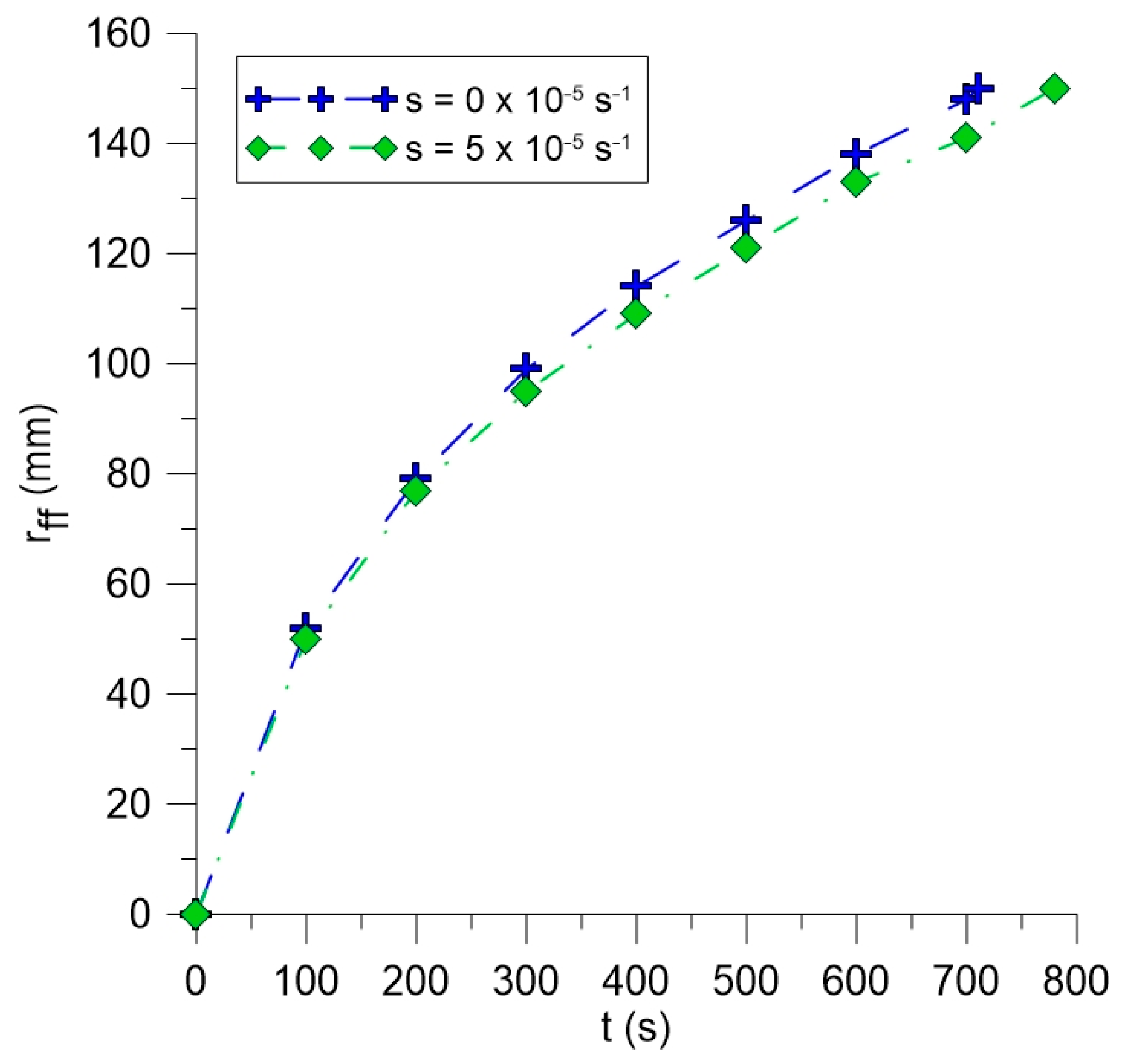
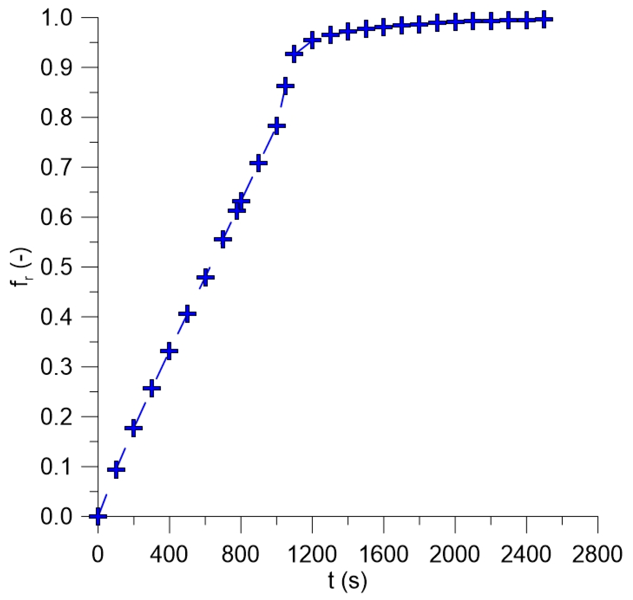
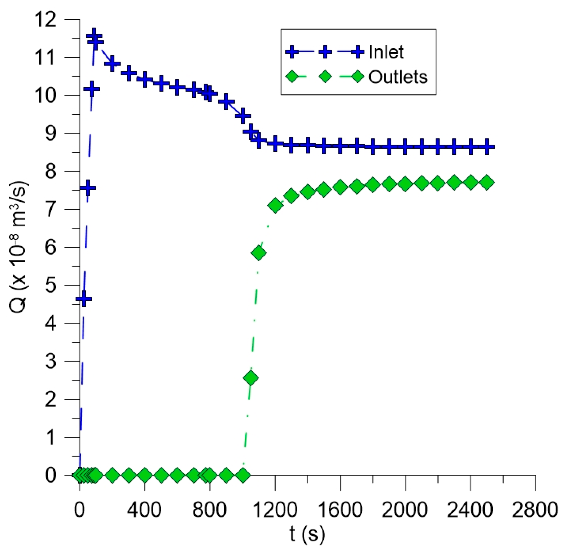
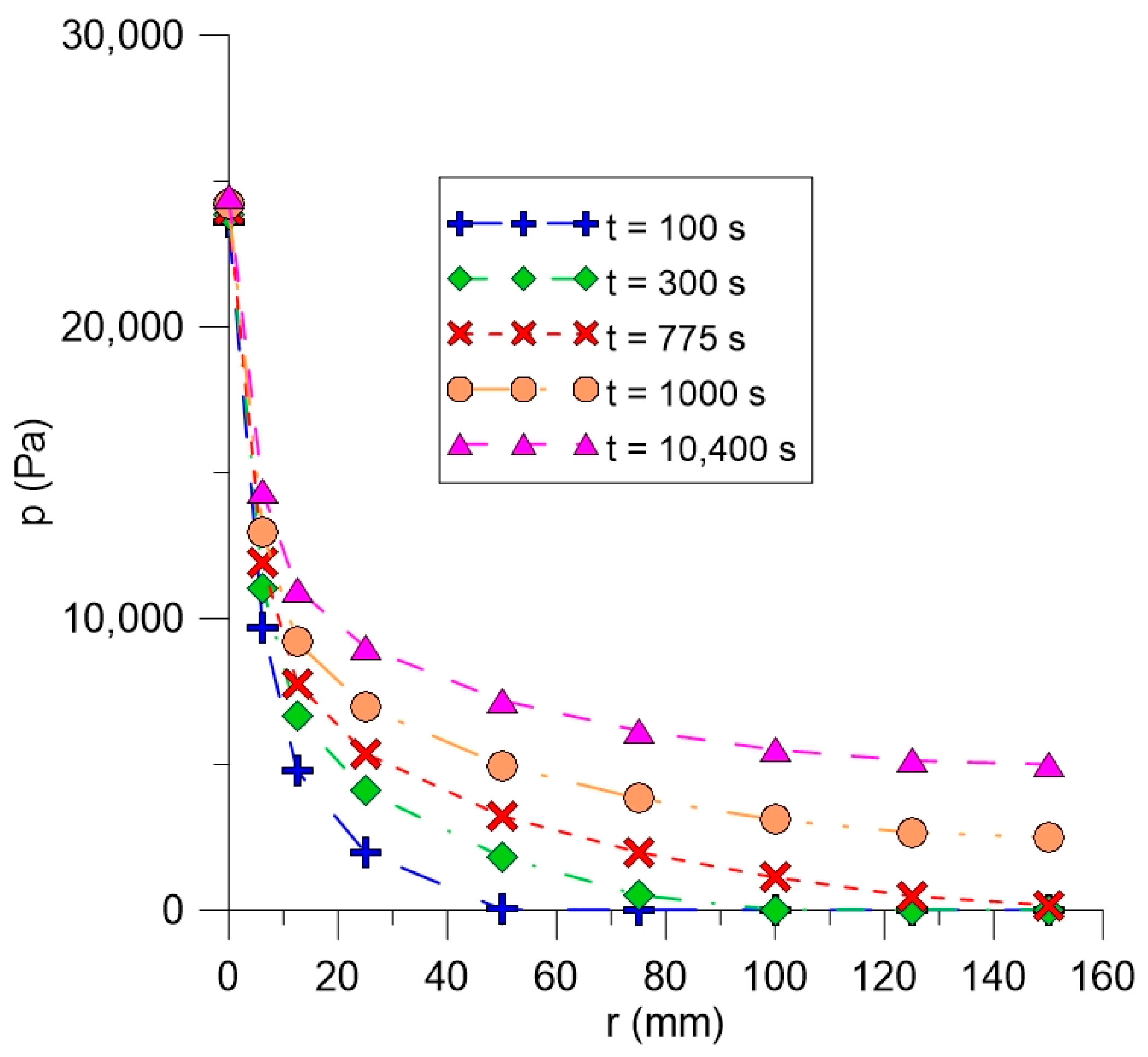
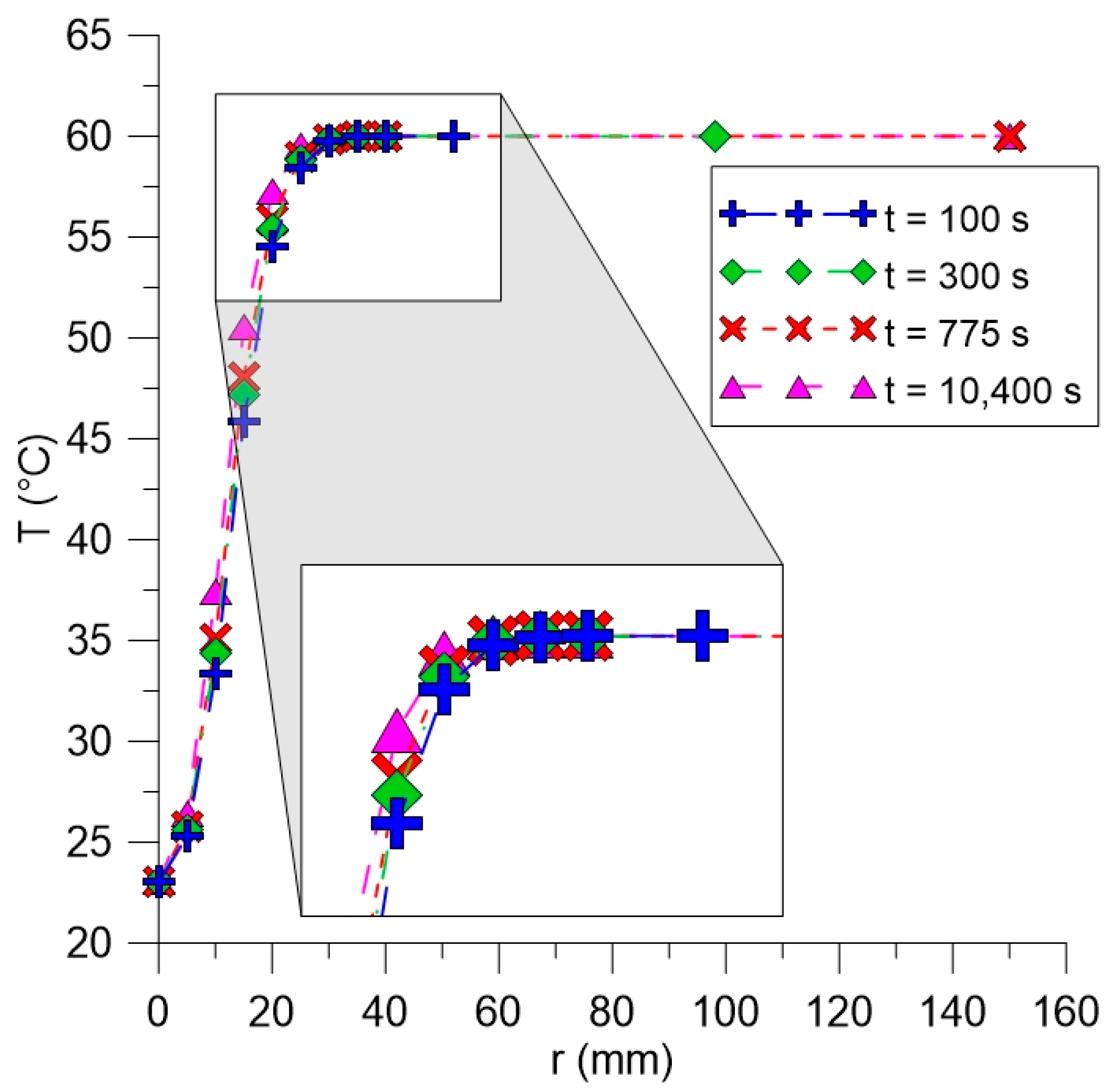
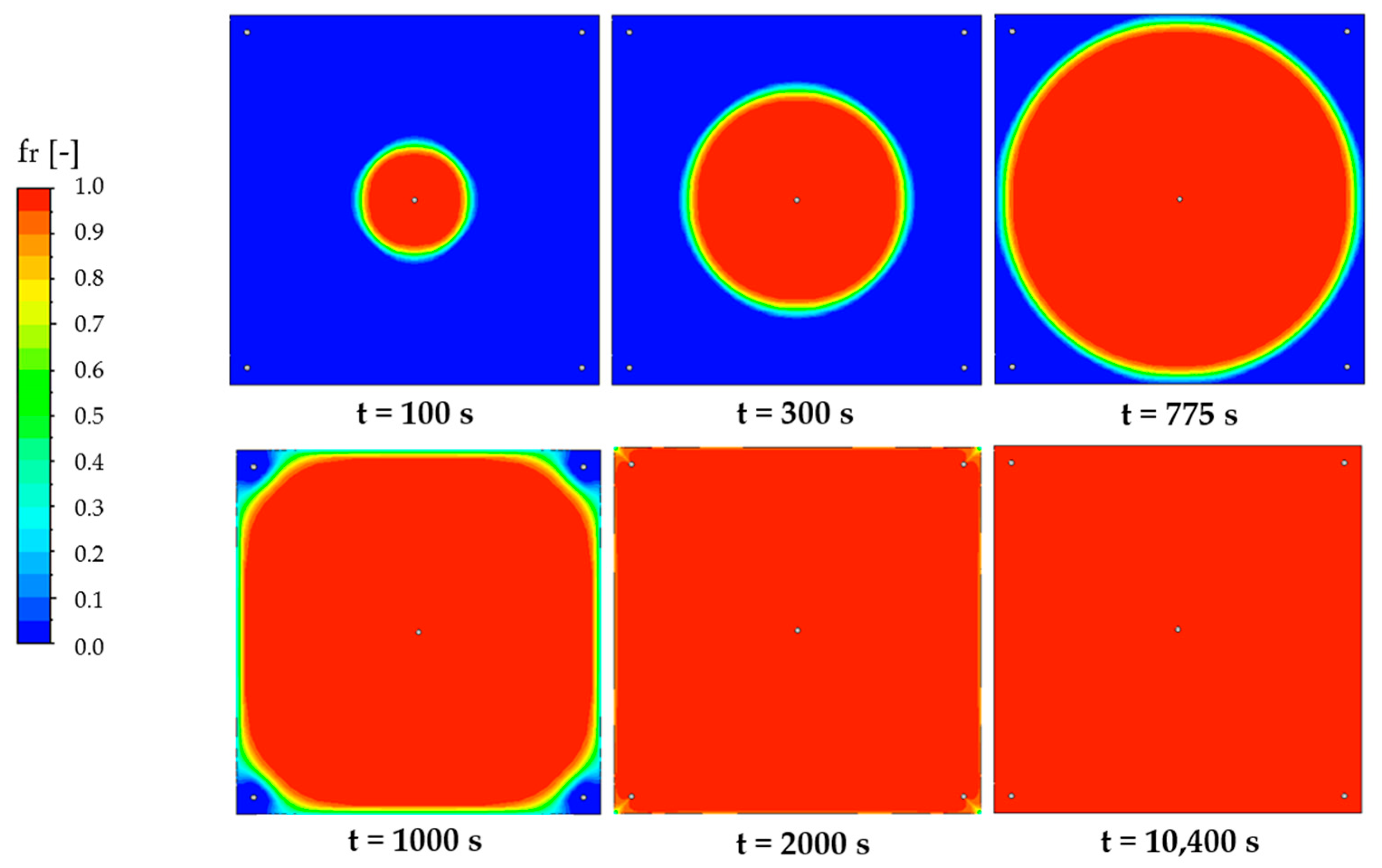
3.1. Thermo-Fluid Dynamic Analysis of Flow

To validate the methodology for constructing the numerical grid, as well as the mathematical model proposed in this article, the experimental data reported by the references [41,46,47] were utilized. These authors used a mold with the same dimensions [46,47], and the same fluid, fibrous reinforcement, and injection conditions [41] used in this paper. For this, the time in which the injected fluid touches the walls of the mold predicted by the numerical simulation was compared with the same parameter obtained experimentally.

In the simulations, a better approximation between the numerical and experimental results for the time in which the flow front reaches the edge of the mold, t_num and t_exp, respectively, was obtained when it was implemented in the model as s = 0.5 × 10⁻⁴ s⁻¹, a condition that was obtained after applying the trial-and-error method. For this situation, the error between the theoretical and experimental parameters was reduced from −9.23% (s = 0.0 × 10⁻⁴ s⁻¹) to −0.64% (s = 0.5 × 10⁻⁴ s⁻¹) (

Table 4. Comparison between the times in which the injected fluid reaches the edge of the mold obtained experimentally and numerically.

s (×10−4 s−1)	texp (s) 1	tnum (s)	Error (%)
0.0	780	708	−9.23
0.5	780	775	−0.64

¹ [41].

), validating the numerical modeling adopted, and evidencing the robustness of the modeling proposed in this research to predict the infiltration of vegetable oil into the fabric fiber.

Figure 8 graphically illustrates the evolution of the flow front of the injected fluid over time, for simulations with the absorption source term equal to 0.0 and 0.5 × 10⁻⁴ s⁻¹. By analyzing this figure, physical coherence is observed. As the value of the absorption source term increases, it is clear that there is a delay in the advance of the flow front over time, especially in more advanced process times, where there is a greater amount of fluid mass injected into the mold and greater absorption of this fluid by the micropores of the fibers.

The evolution of the volumetric fraction of the injected fluid (vegetable oil) inside the mold as a function of time is shown graphically in Figure 9, for simulation with an absorption source term equal to 0.5 × 10⁻⁴ s⁻¹. Analyzing this figure, it is possible to observe an almost linear increase in the volumetric fraction of the injected fluid up to approximately 1000 s. From that moment on, a rapid increase in this variable can be perceived, which reaches a level above 0.99 between 1900 and 2000 s, and then there are subtle increments in the volumetric fraction of the injected fluid over time. The complete stability (steady flow regime) of the volumetric fraction of the injected fluid was reached between 10,300 and 10,400 s, and a volumetric fraction of the injected fluid inside the mold equal to 0.999983 (99.9983%) was observed at this moment of the process. Physically, the linear increase in the volumetric fraction of fluid injected into the mold occurs until approximately the moment when the flow has a predominantly radial behavior. From this moment on, the mixed, linear–radial flow intensifies, and there is then a rapid increase in the volumetric fraction of the injected fluid, until the mold is almost completely filled.

The transient history of the volumetric flow rate of the injected fluid at the inlet and outlets of the mold as a function of time is shown in Figure 10. After analyzing this figure, it is verified that there is a rapid increase in the volumetric flow rate at the inlet gate, at the beginning of the injection, where there is an injection pressure transient (0 to 89 s), reaching the maximum volumetric flow rate of Q = 11.6 × 10⁻⁸ m³/s in 89 s. This can be justified by the fact that, over time, the porous medium present inside the mold is increasingly filled with the injected fluid, causing the resistance to its flow to increase, reducing the inlet volumetric flow rate. This phenomenon is more pronounced in the approximate time of 1000 s, this being the instant in which the vegetable oil reaches the exit gates, and practically stabilizing in times greater than 1500 s.

Finally, still analyzing Figure 10, it can be seen that, for times greater than 10,400 s, the steady flow regime is reached, where the difference between the volumetric flow rate of injected fluid at the inlet, 8.64 × 10⁻⁸ m³/s, and at the outlets (total), 7.74 × 10⁻⁸ m³/s, represents the quantity of injected fluid absorbed by the fibrous reinforcement in the steady flow regime, 0.90 × 10⁻⁸ m³/s. This quantity is numerically equal to the product of the absorption source, 0.5 × 10⁻⁴ s⁻¹, the total volume of the mold, 1.8 × 10⁻⁴ m³, and the volumetric fraction of the injected fluid, 0.999983, being represented by the mass balance expressed by Equation (15), valid for the condition of steady state flow.

$$Q_{in}-Q_{out}=Q_{abs}=s\times \overline{V}\times f_r$$

(15)

where Q_in is the inlet volumetric flow rate of the injected fluid into the mold, Q_out is the outgoing volumetric flow rate of the injected fluid from the mold, Q_abs is the volumetric flow rate of the injected fluid absorbed by the porous medium, and V is the total volume of the mold.

Figure 11 shows the behavior of the gauge pressure in the midline of the mold thickness (1 mm) as a function of the radial position, for the times equal to 100, 300, 775, 1000, and 10,400 s (steady state flow), considering s = 0.5 × 10⁻⁴ s⁻¹. When analyzing the history of this parameter, the existence of physical coherence is verified, where higher pressures near the injection channel and approximately zero pressures are perceived with radii equal to or greater than the radius of the flow front, for times equal to or less than the time in which the injected fluid touches the mold wall (t_num = 775 s). There is a nonlinear behavior of this parameter in the radial direction which increases with the progress of the fluid infiltration in the mold. The reverse is true for the pressure gradients in the radial direction, where there is a decrease in this parameter with the process time.

In Figure 12 is shown the power required to pump the fluid injected into the mold as a function of time, for the condition in which s = 0.5 × 10⁻⁴ s⁻¹, determined by Equation (16). By analyzing the results obtained, it can be seen that there is a rapid increase in the power required at the beginning of the process, in the stage where the injection pressure is variable (up to 89 s), with the peak power (3.14 × 10⁻³ W) observed at 89 s, corresponding to the instant when the peak of the injection volumetric flow rate is verified. A subsequent decrease in the required power is also observed over time, being explained by the reduction in the volumetric flow rate of fluid injection, which is accentuated in the approximate time of 1000 s, corresponding to the instant in which the vegetable oil reaches the exit gates. The stabilization of the required power (steady state) occurred in times greater than 1500 s, and a required power for pumping equal to 2.35 × 10⁻³ W was observed.

$$Pot=Q_{in}\times \left(p_{inj}-p_s\right)$$

(16)

where Pot is the power required to pump the fluid injected into the mold and p_s is the gauge pressure at the mold outlets.

The transient history of the temperature of the injected fluid at the midline of the mold thickness (1 mm) as a function of the radial position, at the instants of 100, 300, 775, and 10,400 s (steady state flow), for s = 0.5 × 10⁻⁴ s⁻¹, is shown in Figure 13. Analyzing this figure, similar temperature profiles can be seen for all the times analyzed, where a rapid heating of the injected fluid is observed with the increase of the radius of the flow front, reaching the mold temperature (60 °C) at r_ff > 30 mm (20% of the maximum radius). It is also observed that there is a slight displacement of the curves to the left for higher process times and r_ff < 30 mm, which is expected, due to the fact that the injected fluid has a longer contact time with the mold, absorbing a greater amount of heat from it and raising its temperature even more.

Figure 14 shows the behavior of the dynamic viscosity of the injected fluid in the midline of the mold thickness (1 mm) as a function of the radial position, for the injection times of 100, 300, 775, and 10,400 s (steady flow regime), for s = 0.5 × 10⁻⁴ s⁻¹. Carefully observing the results predicted by the mathematical model and numerical simulation, similar dynamic viscosity profiles can be verified for all the times analyzed, with a rapid decrease in this parameter with the increase in the flow front radius, reaching a value of 16.5 cP in the mold temperature for r_ff > 30 mm (20% of the maximum radius). Also in this figure, the results of the dynamic viscosity of the injected fluid at the mean line of the mold thickness (1 mm), calculated by Equation (14), as a function of the radial position and process time equal to 10,400 s, are presented. An excellent approximation between these results given by Equation (14) and those verified in the simulation is observed, for the same time, which is expected, since Equation (14) is the input parameter for the mathematical model used in the numerical simulation. The idea is to show that all the calculations of the input parameters are being done correctly, contributing positively to the simulated results.

During the manufacturing process of polymer composites, for example, due to the curing process, the viscosity of the resin decreases due to the increase in the temperature of the resin inside the mold during the infiltration process. However, in this research, the phenomena of curing and crystallization were not considered. Variations in the viscosity of the resin strongly impact the capillary number, which relates the viscous drag forces and the surface tension forces acting through the interface between the resin and the air present in the capillary, as well as in the formation of voids within the mold.

Figure 15 illustrates the distribution of the volumetric fraction of fluid injected into the mold at the process times equal to 100, 300, 775, 1000, and 10,400 s, considering the sorption term s = 0.5 × 10⁻⁴ s⁻¹. Analyzing this figure, a perfectly radial flow is observed until the injected fluid touches the mold walls (t = 775 s), due to the fact that the porous medium is homogeneous, isotropic, and with constant porosity. If the fibrous system had variable porosity, a non-circular distribution would certainly appear on the fluid flow front (fingers). From 775 s of the process, the flow behavior changes from perfectly radial to a mixed radial–linear flow, motivated by the interference of the impermeable mold walls on the fluid flow. There is a tendency for the fluid to be directed to the exit gates located in the vicinity of the vertices of the mold.

Figure 16 illustrates the volumetric fraction field of the injected fluid in the area next to one of the mold outlets. This area is one of the last filling sites, being completely occupied with injected fluid only at high process times, in such a way that these places are potential points of existence of voids in the produced composite. The figure also illustrates the velocity vector field of the injected fluid in this same region. After analyzing this figure, it is observed that the flow of injected fluid is directed to the mold outlet (low pressure zone). No turbulence zones were observed.

Figure 17 illustrates the gauge pressure distribution inside the mold at the process times of 100, 300, 775, 1000 and 10,400 s, considering s = 0.5 × 10⁻⁴ s⁻¹. After analyzing this figure, the existence of maximum pressure in the injection nozzle and a negative pressure gradient with the increase in the radius of the flow front can be verified. It is observed that, in the steady state (10,400 s), there are low pressure zones (almost zero) next to the four mold exits, which is expected, since the gauge pressure at the mold outlet is considered zero. This pressure distribution originates the behavior of the volumetric fraction of the injected fluid inside the mold at the same moment of the infiltration process.

In Figure 18 is illustrated the temperature distribution of the injected fluid in the midline of the mold thickness (1 mm) at the process times equal to 100, 775 and 10,400 s, for s = 0.5 × 10⁻⁴ s⁻¹. Analyzing this figure, very similar fields are verified for all times analyzed, with rapid heating of the injected fluid, reaching the temperature of the mold (60 °C), which is expected, due to the high contact area between the heated mold and the flowing fluid, the low thickness of the mold, and the thermal properties of vegetable oil, which make it a good heat conductor.

3.2. Robustness and Limitations of the Proposed Model

The numerical–mathematical model developed in this article proved to be robust when applied to the production of composites by the RTM process, well-representing the flow of fluid in a porous medium, considering multiphase, three-dimensional, and non-isothermal flow, in a transient regime, and including the phenomenon of sorption of the injected fluid by the micropores of the fibrous reinforcement. This robust model can be applied to evaluate different process parameters, from a porous medium to resin, helping facilitate a deep understanding of the process, which is potentially very important in practical applications and RTM experiments, favoring process optimization. In addition, it becomes possible, as seen, to accurately estimate the permeability of the porous medium, an important parameter for evaluating porous reinforcement.

Despite the advantages of the proposed modeling, it is important to highlight the main limitations of this modeling, which can be improved in future studies:

(a)

Due to the implementation of a constant sorption source term in the model, there is no identification of the saturation limit of the micropores of the fibers;

(b)

The phenomenon of thermal expansion of the mold (mechanical and thermal) is not taken into account;

(c)

The effect of the infiltration of the injected fluid into the individual fibers, such as swelling of the fibers, is not taken into account;

(d)

Different microscopic effects (trapped microvoids, void migration, void compression, and resin microflow) during fiber filling were neglected;

(e)

The dimension, shape, orientation, movement, and accommodation of the fibers, interaction between individual fibers, and deformation of the preform were neglected;

(f)

Curing effects were neglected;

(g)

Modifications in the thickness and deformation of the mold due to the action of pressure inside the closed cavity (mold) and temperature were neglected.

4. Conclusions

In this research, in the context of the production of composites by the RTM process, the thermo-fluid dynamic behavior of the three-dimensional and transient flow of vegetable oil inside a mold filled with fibrous reinforcement (porous medium) was analyzed, including the effect of the absorption of part of the injected fluid by the micropores of the reinforcement. CFD tools were applied, using the commercial software Ansys Icem CFD 2021 R2 and Ansys CFX 2021 R2, where in the former, the geometry and numerical grids were built, while in the latter, the simulations and analysis of the results were carried out.

The simulations performed revealed the good performance of the mathematical model proposed for prediction of the phenomenon, proven by the good approximation between the numerical and experimental results of the time in which the fluid front reaches the edges of the mold. From this comparison, after successive simulations, an absorption source term equal to s = 0.5 × 10⁻⁴ s⁻¹ was obtained, which physically reproduced the injection dynamics observed experimentally, for a mold heated to 60 °C and fluid injected at 23 °C. History curves of several relevant process parameters were plotted, as well as visualizations of the evolution of some relevant property fields, which contributed to a better understanding and consequent optimization of the composite production process by RTM.

The inclusion of the sorption effect of the injected fluid by the fiber (characterized by the presence of a source term in the macroscopic equation of mass conservation) suggests that the delay effect has an influence in the progress of the flow front in a slight way, and has an influence on the pressure drop at the inlet gate. This effect becomes more significant in situations where anisotropy occurs, proving that the exploration of such a line of research has great potential. The authors recommend that future studies should be directed towards the development of a model that includes the sorption term dependent on the direction of fluid flow and capillary pressure between the injected fluid–air inside the mold, which can lead to greater accuracy in simulations related to the manufacture of fiber-reinforced polymer composites using the RTM process.

References

1. Mallick, P.K. Fiber-Reinforced Composites: Materials Manufacturing and Design, 3rd ed.; CRC Press: Boca Raton, FL, USA, 2007; pp. 24–41. [Google Scholar]
2. Trzepieciński, T.; Najm, S.M.; Sbayti, M.; Belhadjsalah, H.; Szpunar, M.; Lemu, H.G. New Advances and Future Possibilities in Forming Technology of Hybrid Metal-Polymer Composites Used in Aerospace Applications. J. Compos. Sci. 2021, 5, 217. [Google Scholar] [CrossRef]
3. Precedence Research. Composites Market. Available online: https://www.precedenceresearch.com/composites-market (accessed on 16 February 2024).
4. Oliveira, I.R. Infiltration of Charged Fluids in Porous Media via RTM Process: Theoretical and Experimental Analysis. Ph.D. Thesis, Federal University of Campina Grande, Paraíba, Brazil, 2014. [Google Scholar]
5. Greve, L.; Pickett, A.K. Delamination Testing and Modelling for Composite Crash Simulation. Compos. Sci. Technol. 2006, 66, 26–816. [Google Scholar] [CrossRef]
6. Ferreira, R. Special Composite Transformation Processes, 1st ed.; Federal Institute of Education, Science and Technology Sul-Rio-Grandense: Sapucaia do Sul, Brazil, 2017; pp. 30–32. [Google Scholar]
7. Osborne Industries. How the Resin Transfer Molding Process Works. Available online: https://www.osborneindustries.com/news/resin-transfer-molding-process-works/ (accessed on 29 September 2023).
8. Delgado, J.M.P.Q.; Lima, A.G.B.; Santos, M.J.N. Transport Phenomena in Liquid Composite Molding Processes, 1st ed.; Springer: Cham, Switzerland, 2019; pp. 1–86. [Google Scholar]
9. Hiremath, P.; Ambiger, K.D.; Jayashree, P.K.; Heckadka, S.S.; Deepak, G.D.; Murthy, B.R.N.; Kowshik, S.; Naik, N. Computational Approach for Optimizing Resin Flow Behavior in Resin Transfer Molding with Variations in Injection Pressure, Fiber Permeability, and Resin Sorption. J. Compos. Sci. 2025, 9, 129. [Google Scholar] [CrossRef]
10. Rudd, C.D.; Long, A.C.; Kendall, K.N.; Mangin, C. Liquid Moulding Technologies: Resin Transfer Moulding, Structural Reaction Injection Moulding and Related Processing Techniques, 1st ed.; Woodhead Publishing: Cambridge, UK, 1997; pp. 294–319. [Google Scholar]
11. Achim, V.; Ruiz, E. Guiding Selection for Reduced Process Development Time in RTM. Int. J. Mater. Form. 2010, 24, 1277–1286. [Google Scholar] [CrossRef]
12. Ruiz, E.; Achim, V.; Soukane, S.; Trochu, F.; Bréard, J. Optimization of Injection Flow Rate to Minimize Micro/Macro-Voids Formation in Resin Transfer Molded Composites. Compos. Sci. Technol. 2006, 66, 475–486. [Google Scholar] [CrossRef]
13. Santos, A.C.M.Q.S.; Monticeli, F.M.; Ornaghi, H.; Santos, L.F.P.; Cioffi, M.O.H. Porosity characterization and respective influence on short-beam strength of advanced composite processed by resin transfer molding and compression molding. Polym. Polym. Compos. 2020, 29, 1353–1362. [Google Scholar] [CrossRef]
14. bin Sulaiman, A.F.F.; binti Abdullah, F.; bin Osman, E.; Rashidi, S.A.; bin Mohd Jais, G. Feasibility Study on a Fabrication Resin Transfer Molding Machine for Aircraft Part (Hinge) Application. In Proceedings of the 7th International Conference and Exhibition on Sustainable Energy and Advanced Materials (ICE-SEAM 2021), Melaka, Malaysia, 23 November 2021. [Google Scholar] [CrossRef]
15. Chen, Z.; Peng, L.; Xiao, Z. Experimental Characterization and Numerical Simulation of Voids in CFRP Components Processed by HP-RTM. Materials 2022, 15, 5249. [Google Scholar] [CrossRef] [PubMed]
16. Martins, F.P.; Santos, L.; Torcato, R.; Lima, P.S.; Oliveira, J.M. Reproducibility Study of the Thermoplastic Resin Transfer Molding Process for Glass Fiber Reinforced Polyamide 6 Composites. Materials 2023, 16, 4652. [Google Scholar] [CrossRef] [PubMed]
17. Yan, C.; Wei, J.; Zhu, Y.; Xu, H.; Liu, D.; Chen, G.; Liu, X.; Dai, J.; Lv, D. Preparation and properties of carbon fiber reinforced bio-based degradable acetal-linkage-containing epoxy resin composites by RTM process. Polym. Compos. 2023, 44, 4081–4094. [Google Scholar] [CrossRef]
18. Zhang, C.; Sun, T.; Xu, J.; Shi, X.; Zhang, G. Effect of Mold on Curing Deformation of Resin Transfer Molding-Made Textile Composites. Polym. Compos. 2023, 44, 7599–7610. [Google Scholar] [CrossRef]
19. Aldhahri, K.S.; Klosterman, D.A. Additively Manufactured Resin Transfer Molding (RTM) Plastic Tooling for Producing Composite T-joint Structures. Prog. Addit. Manuf. 2025, 10, 2283–2301. [Google Scholar] [CrossRef]
20. Wang, X.; Xue, F.; Gu, X.; Xia, X. Simulation of Frost-Heave Failure of Air-Entrained Concrete Based on Thermal–Hydraulic Mechanical Coupling Model. Materials 2024, 17, 3727. [Google Scholar] [CrossRef] [PubMed]
21. Zhao, F.; Liu, X.; Zhao, J.; Feng, T.; Guo, W. Plant fiber-reinforced composites based on injection molding process: Manufacturing, service life, and remanufacturing. Polym. Compos. 2024, 45, 4876–4899. [Google Scholar] [CrossRef]
22. Song, X.; Grimsley, B.W.; Hubert, P.; Cano, R.J.; Loos, A.C. VARTM Process Modeling of Aerospace Composite Structures. In Proceedings of the American Society for Composites, 17th Technical Conference, West Lafayette, IN, USA, 21–23 October 2002. [Google Scholar]
23. Isoldi, L.A.; Oliveira, C.P.; Rocha, L.A.O.; Souza, J.A.; Amico, S.C. Three-Dimensional Numerical Modeling of RTM and LRTM Processes. J. Braz. Soc. Mech. Sci. Eng. 2012, 34, 105–111. [Google Scholar] [CrossRef]
24. Oliveira, I.R.; Amico, S.C.; Souza, J.A.; Lima, A.G.B. Resin Transfer Molding Process: A Numerical and Experimental Investigation. Int. J. Multiphysics 2013, 7, 125–135. [Google Scholar] [CrossRef]
25. Moumen, A.E.; Saouab, A.; Imad, A.; Kanit, T. Towards a Numerical Modeling of the Coupling Between RTM Process and Induced Mechanical Properties for Rigid Particle-Filled Composites. J. Adv. Manuf. Technol. 2023, 125, 1251–1270. [Google Scholar] [CrossRef]
26. Alotaibi, H.; Abeykoon, C.; Soutis, C.; Jabbari, M. Numerical Simulation of Two-Phase Flow in Liquid Composite Moulding Using VOF-Based Implicit Time-Stepping Scheme. J. Compos. Sci. 2022, 6, 330. [Google Scholar] [CrossRef]
27. Landi, D.; Vita, A.; Germani, M. Interactive Optimization of the Resin Transfer Molding Using a General-Purpose Tool: A Case Study. Int. J. Interact. Des. Manuf. 2020, 14, 295–308. [Google Scholar] [CrossRef]
28. Goh, K.W.; Algot, K.K.; Laxmaiah, G.; Babu, P.R.; Vodnala, V.P.; Zainul, R. Experimental analysis, simulation, and evaluation of process parameters of GFRP composites produced through resin transfer molding. Adv. Manuf. Polym. Compos. Sci. 2025, 11, 2441629. [Google Scholar] [CrossRef]
29. Yang, W.; Lu, S.; Xiang, L.; Liu, W. Simulation of Non-Isothermal Resin Transfer Molding Process Cycle and Optimization of Temperature System. J. Reinf. Plast. Compos. 2019, 38, 3–14. [Google Scholar] [CrossRef]
30. Pazdzior, P.; Szczepanik, M. Resin Flow Simulation During the RTM Method of Composites Production. Int. J. Mod. Manuf. Technol. 2021, 13, 125–133. [Google Scholar] [CrossRef]
31. Seuffert, J.; Rosenberg, R.; Kärger, L.; Henning, F.; Kothmann, M.H.; Deinzer, G. Experimental and Numerical Investigations of Pressure-Controlled Resin Transfer Molding (PC-RTM). Adv. Manuf. Polym. Compos. Sci. 2020, 6, 154–163. [Google Scholar] [CrossRef]
32. Shi, F.; Zhao, Z.; Dong, X. An Improved Method of Numerical Simulation of Resin Transfer Molding for Resin-Based Composite Materials Based on Unstructured Grid. Adv. Intell. Syst. Res. 2018, 159, 280–287. [Google Scholar]
33. Soares, L.L. Numerical Simulation of the RTM Process for the Infiltration of Thick Reinforcements Considering the Variation of Resin Viscosity as a Function of Temperature and Time. Master’s Dissertation, Federal University of Rio Grande, Rio Grande, Brazil, 2017. [Google Scholar]
34. Yang, H.; Hsu, C.C.; Hsu, C.H. Three Dimensional Numerical Simulations for Wet-RTM Process. In Proceedings of the 35th International Conference of the Polymer Processing Society (PPS-35), Cesme-Izmir, Turkey, 26–30 May 2019. [Google Scholar] [CrossRef]
35. Shahnazari, M.R.; Abassi, A. Numerical Modeling of Mold Filling and Curing in Non-Isothermal RTM Process. Int. J. Eng. Trans. A Basics 2004, 17, 395–404. [Google Scholar]
36. Oliveira, J.S.; Carvalho, L.H.; Delgado, J.M.P.Q.; Lima, A.G.B.; Pereira, A.S.; Franco, C.M.R.; Chaves, F.S. Applying Resin Radial Injection for Manufacturing Fiber-Reinforced Polymer Composite: Advanced Mathematical Modeling and Simulation. Polymers 2024, 16, 3525. [Google Scholar] [CrossRef] [PubMed]
37. Santos, P.H.J.; Santos, G.O.; Andrade, M.C.; Santana, P.L.; Pagano, R.L. Mesh Convergence Study for Gas-Liquid Flow Analysis Using the GCI Method. Braz. J. Dev. 2022, 8, 32586–32599. [Google Scholar] [CrossRef]
38. Gomez, R.S.; Porto, T.R.N.; Magalhães, H.L.F.; Moreira, G.; André, A.M.M.C.N.; Melo, R.B.F.; Lima, A.G.B. Natural Gas Intermittent Kiln for the Ceramic Industry: A Transient Thermal Analysis. Energies 2019, 12, 1568. [Google Scholar] [CrossRef]
39. Celik, I.B.; Ghia, U.; Roache, P.; Freitas, C.J.; Coleman, H.; Raad, P.E. Procedure for Estimation and Reporting of Uncertainty Due to Discretization in CFD Applications. J. Fluids Eng. 2008, 130. [Google Scholar] [CrossRef]
40. Ward, J.C. Turbulent Flow in Porous Media. J. Hydraul. Div. 1964, 90, 1–12. [Google Scholar] [CrossRef]
41. Luz, F.F. Comparative Analysis of Fluid Flow in RTM Experiments Using Commercial Applications. Master’s Dissertation, Federal University of Rio Grande do Sul, Porto Alegre, Brazil, 2011. Available online: https://lume.ufrgs.br/handle/10183/62075?locale-attribute=en&show=full (accessed on 28 March 2024).
42. Azo Materials. E-Glass Fibre. ArticleID = 764. 2024. Available online: https://www.azom.com/properties.aspx? (accessed on 15 April 2024).
43. Zhou, Z.; Jiang, B.; Chen, X.; Jiang, F.; Jiang, Y. Rheological Behavior and Process Prediction of Low Viscosity Epoxy Resin for RTM. J. Wuhan Univ. Technol. Mater. Sci. Ed. 2014, 29, 1078–1082. [Google Scholar] [CrossRef]
44. Rojas, E.E.G.; Coimbra, J.S.R.; Telis-Romero, J. Thermophysical Properties of Cotton, Canola, Sunflower and Soybean Oils as a Function of Temperature. Int. J. Food Prop. 2013, 16, 1620–1629. [Google Scholar] [CrossRef]
45. Microelectronics Heat Transfer Laboratory. Fluid Properties Calculator. 2024. Available online: http://www.mhtl.uwaterloo.ca/old/onlinetools/airprop/airprop.html (accessed on 15 April 2024).
46. Luz, F.F.; Amico, S.C.; Cunha, A.L.; Barbosa, E.S.; Lima, A.G.B. Applying Computational Analysis in Studies of Resin Transfer Moulding. Def. Diff. Forum 2012, 326, 158–163. [Google Scholar] [CrossRef]
47. Luz, F.F.; Amico, S.C.; Souza, J.A.; Barbosa, E.S.; Lima, A.G.B. Resin Transfer Molding Process: Fundamentals, Numerical Computation and Experiments. In Numerical Analysis of Heat and Mass Transfer in Porous Media. Series: Advanced Structured Materials, 1st ed.; Delgado, J.M.P.Q., Barbosa de Lima, A.G., Vázquez da Silva, M., Eds.; Springer: Berlin/Heidelberg, Germany, 2012; Volume 27, pp. 121–151. [Google Scholar] [CrossRef]
Figure 1. View in (a) perspective and of (b) the bottom of the mold under study.
Jmmp 09 00243 g001
Figure 2. Bottom view of the optimized numerical mesh.
Jmmp 09 00243 g002
Figure 3. Injection point positioned near the base of the numerical mesh (a) and detail A of this injection point (b).
Jmmp 09 00243 g003
Figure 4. One of the four exit points near the base of the numerical mesh (a) and detail B of this exit point (b).
Jmmp 09 00243 g004
Figure 5. Side view of the numerical mesh.
Jmmp 09 00243 g005
Figure 6. Schematic representation of the resin flow in the RTM process, with emphasis on the phenomenon of absorption of the injected fluid by the fibrous reinforcement.
Jmmp 09 00243 g006
Figure 7. The mold studied, with emphasis on the injection point (A) and the four exit points (B–E).
Jmmp 09 00243 g007
Figure 8. Evolution of the fluid flow front with time for the mold heated to 60 °C, and different absorption terms.
Jmmp 09 00243 g008
Figure 9. Evolution of the volumetric fraction of fluid injected into the mold as a function of time.
Jmmp 09 00243 g009
Figure 10. Evolution of the volumetric flow rate of the fluid injected at the inlet and outlets of the mold as a function of time.
Jmmp 09 00243 g010
Figure 11. Evolution of gauge pressure in the midline of the mold thickness as a function of the radial position, at different process times.
Jmmp 09 00243 g011
Figure 12. Evolution of the power required for pumping the injected fluid as a function of time.
Jmmp 09 00243 g012
Figure 13. Evolution of the temperature of the injected fluid in the midline of the mold thickness as a function of the radial position, at different process times.
Jmmp 09 00243 g013
Figure 14. Evolution of the dynamic viscosity of the injected fluid in the midline of the mold thickness as a function of the radial position, at different process times.
Jmmp 09 00243 g014
Figure 15. Distribution of the volumetric fraction of fluid injected into the mold at different process times.
Jmmp 09 00243 g015
Figure 16. Distribution of the volumetric fraction (a) and velocity vector field (b) of the fluid injected into the mold in the region near the vertex of the mold (t = 2000 s).
Jmmp 09 00243 g016
Figure 17. Gauge pressure distribution inside the mold for different process times.
Jmmp 09 00243 g017
Figure 18. Temperature distribution of the fluid injected into the mold at different process times.
Jmmp 09 00243 g018