Comprehensive Prediction Model for Analysis of Rolling Bearing Ring Waviness

Abstract

The objective of this study was to identify surface geometric deviations that may adversely affect the operational properties of bearings, including vibration, noise, and service life. A comprehensive prediction model is presented that combines a fundamental trend expressed by a power function with periodic oscillations, whose influence gradually diminishes with exponential decay. The model was calibrated using the experimental data obtained from 17 industrial RA-608-338 rolling bearing rings manufactured from high-carbon, low-alloy 100Cr6 steel. An excellent goodness-of-fit (R² exceeding 0.98) and minimal root-mean-square error (RMSE) were achieved. The proposed procedure provides a clear physical interpretation of the model’s subcomponents, while facilitating straightforward implementation in real production processes for continuous quality control and predictive maintenance purposes. This paper also includes a detailed description of the methodology, data processing, experimental results, comparison of multiple model variants, interactive visualization of the results on a logarithmic scale, and recommendations for practical application.

1. Introduction

Surface waviness in rolling bearing raceways represents a fundamental quality parameter that governs vibration behaviour, acoustic emissions, and operational wear patterns in mechanical assemblies. This geometric characteristic differs markedly from surface roughness—while roughness encompasses high-frequency microscopic surface features, waviness encompasses mid-frequency deviations that exert substantial influence on overall bearing dynamics.

The foundational understanding of waviness-bearing performance relationships emerged through Palmgren’s seminal research [1], which established quantitative connections between geometric precision and service life. Palmgren’s investigations revealed how minute geometric variations create disproportionate effects on contact zone stress fields, fundamentally altering fatigue life characteristics. This pioneering work established the critical principle that geometric fidelity directly governs bearing operational performance.

Harris and Kotzalas [2] subsequently expanded this knowledge base through their comprehensive examination of geometric deviation types in “Essential Concepts of Bearing Technology.” Their systematic analysis identified specific waviness frequency bands that produce the most pronounced performance impacts, while simultaneously introducing structured measurement methodologies emphasizing practical industrial applications.

The measurement science foundation was established by Eschmann et al. [3], whose systematic evaluation of roundness and waviness measurement techniques provided the first comparative accuracy assessment across different methodological approaches. Their work created a standardized measurement framework prioritizing result consistency and reproducibility across different laboratory environments.

Tallian [4] advanced the field significantly by creating a comprehensive geometric deviation classification system that correlated specific waviness patterns with distinct bearing failure mechanisms. His “Failure Atlas for Hertz Contact Machine Elements” became an essential diagnostic reference, enabling practitioners to identify geometric quality issues and trace them to their failure consequences.

Statistical modelling approaches gained prominence through Lundberg and Palmgren’s [5] introduction of Weibull distribution concepts for bearing failure analysis. Their research demonstrated how geometric variations modify distribution parameters, establishing the statistical foundation for contemporary bearing reliability prediction methodologies and highlighting waviness effects on probabilistic life characteristics.

Measurement technology experienced a paradigm shift with Donaldson’s [6] laser interferometry applications, achieving submicron measurement capabilities with resolution exceeding 10 nm precision. This technological breakthrough enabled previously impossible analysis of high-frequency waviness components, opening new frontiers in precision bearing quality assessment.

Whitehouse [7] revolutionized surface analysis through sophisticated filtering algorithms that separate frequency components within surface variation spectra. His spectral analysis methods enabled manufacturers to identify specific production processes responsible for waviness generation, creating direct links between manufacturing parameters and resulting surface characteristics. Reason [8] complemented these advances by optimizing contact measurement approaches, developing innovative probe designs that minimise surface deformation during measurement procedures. Butler [9] addressed thermal stability concerns by developing compensation techniques for temperature-induced measurement errors, ensuring reliable results across varying industrial environmental conditions.

Real-time quality monitoring capabilities emerged through Evans et al.’s [10] revolutionary manufacturing process integration systems. Their approach enables instantaneous geometric deviation detection and correction, substantially improving production consistency while reducing waviness variability in manufacturing environments.

Mathematical modelling evolution has produced increasingly sophisticated predictive capabilities. Wang et al. [11] developed the first comprehensive analytical framework for predicting waviness effects on aerostatic bearing static characteristics. Their elastic deformation-based model enables quantitative prediction of stiffness and load capacity variations as functions of waviness parameters, providing engineers with practical design optimisation tools.

Dynamic modelling capabilities advanced through Liu et al.’s [12] time-dependent friction analysis for angular contact bearings experiencing waviness errors. Their finite element-based numerical approach predicts vibration characteristics for bearings with various geometric deviations, establishing quantitative relationships between waviness patterns and resulting vibrational responses. Kania [13] extended modelling sophistication by incorporating multiphysics effects including thermal phenomena and lubricant property variations. This comprehensive modelling approach enables bearing behaviour prediction across broad operational parameter ranges while demonstrating significant waviness influences on thermal performance characteristics.

Probabilistic modelling methodologies were pioneered by Sadeghi et al. [14], who introduced stochastic approaches for characterizing random waviness components and their life cycle effects. This methodology enables uncertainty quantification in bearing performance predictions and tolerance optimisation based on statistical principles. Ioannides and Harris [15] developed sophisticated statistical frameworks for fatigue damage analysis incorporating geometric variations, demonstrating waviness effects on stress distributions and fatigue crack initiation probabilities within contact regions.

Artificial intelligence integration has transformed waviness analysis capabilities through multiple breakthrough applications. Zhao et al. [16] introduced convolutional neural network approaches for automated waviness classification based on measured surface profiles. Their system demonstrates classification accuracy exceeding 95 % while simultaneously identifying specific manufacturing problems responsible for waviness formation, enabling real-time quality control implementation.

Yang et al. [17] created hybrid predictive models combining physics-based equations with machine learning algorithms for bearing reliability assessment. Their methodology enables remaining useful life prediction based on measured waviness characteristics with accuracy substantially exceeding traditional approaches, facilitating predictive maintenance strategy implementation. Lei et al. [18] expanded deep learning applications into time-series vibration analysis for bearings exhibiting waviness, developing recurrent neural networks that identify degradation patterns and optimise bearing replacement timing.

Gupta et al. [19] implemented genetic algorithm approaches for manufacturing parameter optimisation using measured waviness characteristics as feedback. Their automated system minimizes waviness while maintaining economic production efficiency, demonstrating practical artificial intelligence applications in bearing manufacturing.

Automotive industry requirements have driven specialized waviness control methodology development. Zmarzły [20] conducted comprehensive technological heredity analysis in rolling bearing ring production using waviness measurements as primary indicators, achieving 30% reduction in geometric characteristic variability through optimised manufacturing parameters. His subsequent research [21] developed multidimensional mathematical wear prediction models using bearing-generated vibrations, enabling accurate wear forecasting under realistic operational conditions for predictive maintenance applications.

Šafář et al. [22] created optimisation methodologies for automotive steel bearing ring dimensions, integrating waviness analysis with cost optimisation to achieve balanced quality-economic efficiency relationships. Their approach demonstrates practical waviness control implementation in cost-sensitive manufacturing environments.

Aerospace applications have catalyzed advanced material innovation approaches. Yin et al. [23] introduced groundbreaking nanoengineering techniques for bearing steel surfaces using ultrasonic shot peening processes. Their methodology creates controlled gradient nanostructures that substantially enhance wear resistance while simultaneously reducing surface waviness through microstructural homogenization effects. Dong et al. [24] extended these findings through M50 bearing steel investigations with gradient nanograin structures, achieving substantial waviness amplitude reductions through combined surface microstructural homogenization and residual stress optimisation.

Paladugu and Hyde [25] investigated microstructural influences on residual austenite and stress evolution during contact fatigue under mixed lubrication conditions. Their findings demonstrated that refined microstructures substantially extend rolling element service life while reducing waviness sensitivity. Yu et al. [26] conducted rolling bearing reliability analysis considering failure mode correlations, demonstrating waviness effects on multiple degradation mechanisms and optimizing maintenance strategies for energy sector applications.

Contemporary signal processing methodologies have been revolutionized through Liu et al.’s [27] signal coherence theory applications for waviness-induced bearing vibration analysis. Their wavelet transform-based approach enables local waviness change identification while correlating these changes with dynamic bearing characteristics, providing real-time condition monitoring capabilities.

Cheng et al. [28] developed enhanced vibration analysis models for deep groove bearings with localized and distributed faults under variable speed conditions. Their methodology enables vibration response prediction for bearings exhibiting complex waviness patterns under realistic operational scenarios. Feng et al. [29] created advanced bearing defect detection methods using digital twin technology and adversarial graph networks, enabling real-time condition monitoring and failure prediction with exceptional accuracy.

Shestakov and Qodirov [30] introduced correlation-functional methodologies and signal processing algorithms specifically for rolling bearing fault diagnosis. Their approach enables effective waviness signal separation from other vibration sources, enhancing diagnostic accuracy in complex mechanical systems.

Despite substantial research progress, significant knowledge gaps persist in bearing waviness understanding. Current studies predominantly address isolated waviness aspects rather than developing comprehensive prediction models that integrate multiple waviness characteristics into unified frameworks with clear physical interpretation. Existing approaches frequently require specialized equipment and expertise, constraining implementation in typical production environments.

This investigation addresses these limitations through comprehensive prediction model development that combines physical interpretability with practical implementation feasibility. The proposed model integrates multiple waviness characteristics into a unified framework suitable for industrial deployment without requiring specialized software or complex computational infrastructure, with validation using authentic industrial bearing production data.

2. Materials and Methods

2.1. Bearing Material

RA-608-338 rolling bearing rings were fabricated from high-carbon, low-alloy 100Cr6 steel with a carbon content of approximately 0.95 to 1.05 % and a chromium content of approximately 1.3 to 1.6 %. The elevated carbon content ensures that subsequent to heat treatment, which encompasses quenching and tempering, the rings attain a hardness of 60.5 HRC with a tolerance range of ±2 HRC. Chromium enhances the toughness, hardness, and wear resistance of the alloy steel. This specific composition achieves an optimal balance between the hardness requisite for ensuring wear resistance and the toughness to prevent brittleness and premature bearing failure. This combination of properties is crucial for ensuring the longevity and reliability of bearings in demanding applications such as industrial machinery and automotive components.

2.2. Sample Preparation

Prior to thermal processing, the rings were subjected to ultrasonic cleaning to remove impurities, oils, and manufacturing residues. This procedure ensured that undesirable reactions that could potentially affect the final properties of the material did not occur during the quenching process. Subsequently, the rings were quenched in a salt bath, which facilitated more rapid and uniform cooling than traditional oil quenching. This quenching technique contributes to achieving a homogeneous structure and enhances the overall hardness of the material. Following the tempering process, which is crucial for reducing the internal stress and increasing the toughness, the rings were machined by turning and grinding on a MIKROSA SASL 5 centreless grinding machine.

To establish the cutting speed, a value of 67.5 m·s⁻¹ was determined as optimal for achieving the required surface quality.

The grinding process was conducted in three distinct stages, each with a specific objective of roughing, finishing grinding, and superfinishing.

Roughing: In this initial stage, the major shape variations and surface imperfections were removed. Careful attention was paid during roughing to ensure that the components were as close as possible to the desired dimensions.

Finishing grinding: This stage aims to achieve the desired geometry and improve surface quality. The grinding wheels utilized had finer grains, which contributed to a smoother surface.

Superfinishing: This final stage of grinding ensures a very fine surface and minimizes the waviness. Superfinishing is essential to ensure optimum bearing function, as it eliminates microscopic irregularities that could lead to excessive wear or failure.

2.3. Measurement Methodology

For the measurement of ring waviness, a high-precision compact commercial measuring instrument, MAHR MMQ150 (Figure 1), was utilized to measure deviations in shape and position, specifically roudness, waviness, cylindricity, parallelism, and throw, capable of providing highly accurate and repeatable results. In engineering practice, the measurement of roudness is significant because it affects the mechanical accuracy of the component (seating surfaces and mounting tolerances). Waviness measurement is crucial for identifying the bearing noise and vibration (higher waviness correlates with increased rotational noise). Compared to alternative methods and other commercial instruments, the combination of roudness and waviness in one measurement represents a significant timesaving and, most importantly, a comprehensive analysis of the measurement results. The MAHR MMQ150 employs the rotary reference method, which is the standard for measuring roudness and related deviations. Waviness measurements were based on an advanced FFT spectral analysis method. Waviness is principally a low-frequency component of the roudness profile, and the results are recorded using high-precision sensors with resolutions down to 0.01 µm. Gaussian and Fourier filters were applied to separate the roudness and waviness results. Roudness contains both global variations (low frequencies) and waviness components (mid-frequencies). The filters eliminate low-frequency components and retain only wavy structures. FFT analysis identifies the dominant wavelengths by converting the measured signal into a frequency spectrum in which the dominant waviness frequencies are visible (e.g., a dominant waviness with x-peaks implies a surface oscillation with x-waves around the circumference of the ring). The instrument allows not only the quantification of shape deviations, but also the diagnosis of manufacturing problems that cause unwanted vibrations/machining vibrations or grinding defects, as well as bearing and ring noise.

The MAHR MMQ150 measuring device was configured with a precision tip with a radius of 2 μm and a contact force of 0.75 mN. The measuring arm was positioned perpendicular to the orbital surface, and the ring was mounted on a precision spindle with a runout of less than 0.05 μm. The measurement radius was set to the nominal orbit radius minus 0.3 mm to ensure consistent contact with the orbit surface while avoiding edge effects.

Roundness measurements were performed at three specific heights on each bearing ring to provide a comprehensive characterisation of the geometric deviations. The measurement protocol was designed according to ISO 492:2014 [31] standards for rolling bearing tolerances and followed the recommendations provided in ISO 1132-1:2000 [32] for rolling bearing measurement procedures.

Primary measurements of roundness were taken at half the height of the ring orbit, specifically at 50% of the ring width (measured from either face). This location was chosen because it represents the critical contact zone where the rolling elements interact with the orbit during the operation. At this position, any geometric variations have the most significant impact on the bearing performance, vibration characteristics, and life.

Additional measurements were performed at 25% and 75% of the ring width to assess the consistency of the geometric characteristics across the entire orbit width. These measurements help identify potential manufacturing issues such as taper, barrel deviations, or localized geometric irregularities that may not be apparent from a single measurement plane.

The 1–500 upr filter was specifically designed to isolate waviness components most relevant for bearing performance prediction:

• Lower limit (1 upr): Eliminates shape deviations and centring errors not relevant to waviness analysis
• Upper limit (500 upr): Retains all relevant waviness information while eliminating surface roughness components and measurement noise
• Wavelength range: For RA-608-338 bearings (Ø22 mm), corresponds to 69 μm–0.14 μm wavelengths
• Implementation: Combined Gaussian and Fourier filtering techniques with smooth transient characteristics

The sample set of selected rolling bearing rings comprised of 17 rings that were automatically adjusted, clamped, centred, and measured under specific conditions. These conditions were carefully selected to minimise the influence of external factors, such as temperature and vibration.

The acquired data were analyzed using the advanced software packages Minitab (Minitab v20.4), MATLAB (R2015b), and Python (3.13.1). Minitab was employed for statistical analyses, including analysis of variance (ANOVA), which facilitated the assessment of the effects of various parameters on the waviness and roudness of the rings. MATLAB was used for the advanced signal processing and visualization of the acquired data. Python was selected as the contemporary general-purpose programming language to process the generated data. The combination of these software tools enabled comprehensive analysis and interpretation of the results, facilitating the identification of key factors influencing the corrugation and overall quality of the rings. This analysis contributed to the formulation of recommendations for optimizing the manufacturing processes.

Surface roughness measurements were performed using a Mitutoyo SJ-410 portable surface roughness tester calibrated according to ISO 4287:1997 [33] and ISO 4288:1996 [34]. The instrument was equipped with a diamond tip with a tip radius of 2 μm and a contact force of 0.75 mN, identical to the specifications used for ovality measurements to ensure consistency under surface contact conditions. Roughness measurements were performed using the following standardized parameters:

• evaluation length (ln) 4.0 mm;
• sampling length (lr) 0.8 mm;
• number of sampling lengths 5;
• tip speed 0.5 mm/s;
• Gaussian filter according to ISO 11562:1996 [35].

Roughness measurements were taken at six evenly spaced circumferential positions around each bearing ring to account for potential variations owing to the manufacturing processes. Three measurements were taken at each circumferential position:

• in the axial direction (parallel to the axis of the ring);
• in the circumferential direction (tangential to the orbit);
• in the radial direction (perpendicular to the surface of the orbit).

Hardness measurements were performed using a Wilson Rockwell 574 hardness tester calibrated according to the ASTM E18-20 standards. The instrument was equipped with a diamond cone (Brale indenter) to measure the HRC scale, which is the standard scale for hardened bearing steel.

Prior to the hardness testing, bearing ring samples were prepared according to the requirements of ASTM E18-20 [36]:

• surface grinding to achieve a surface roughness Ra < 0.4 μm;
• acetone cleaning to remove any surface contamination;
• clamping in a rigid fixture to ensure perpendicular loading;
• temperature stabilization of 23 ± 2 °C for a minimum of 30 min.

Hardness measurements were performed on the HRC scale using the following parameters.

• preload 98.07 N (10 kgf);
• total load 1471 N (150 kgf);
• load time 2–8 s;
• residence time under total load 2–6 s.

For each bearing ring, hardness measurements were taken at 12 equally spaced locations around the circumference, with measurements taken on the orbital surface at the same axial position used for the primary ovality measurement. This approach provides a direct correlation between the hardness and geometry measurements. The hardness tester was calibrated daily using certified reference blocks with known hardness values (60 ± 1 HRC). The repeatability of the measurements was verified by taking five consecutive measurements at the same location, with an acceptance criterion of standard deviation < 0.5 HRC.

2.4. Mathematical Model

Signal measurements are encountered in numerous applications, such as production process monitoring, wherein two primary dynamics are observed. A long-term trend is present, representing systematic changes (e.g., aging, wear, and tear of equipment) alongside periodic oscillations, which are attributable to cyclic processes or mechanical vibrations, the amplitude of which may diminish over time. This combination can be expressed as the sum of two components: the trend and oscillatory components. This concept is predicated on the general methodology of signal decomposition, which is frequently employed in time-series analyses.

2.4.1. Formulation of the Proposed Model

Therefore, the proposed model is predicated on a combination of two components that elucidate the dynamics of measured values in real production processes. The equation for the model assumes the following form (1):

$${\lambda }_n=A·n^{\beta }+C·e^{(-D·n)}·\cos \left({\displaystyle \frac{2\pi }{T}}·n+\phi \right)$$

(1)

where:

λ_n—predicted value of the measured parameter for the i-th ring at the measuring point n; predicted value of the measured parameter for the i-th ring at the measuring point n.

The model attempts to capture the dominant observable surface texture dynamics using a mathematical structure whose components have direct physical interpretation. The model comprises of two fundamental parts that represent two distinct types of phenomena that shape the final ring geometry. The first is the component A·n^β, which describes the long-term, systematic, and monotonic changes in the surface profile. The choice of power function is not random. Power laws often appear in natural and engineering systems where processes exhibit scale invariance or long-term memory effects. In the context of grinding, this component represents several concurrent phenomena. This may be due to the non-linear wear of the grinding wheel, where its cutting ability changes gradually along the grinding path. Another phenomenon may be thermal drift in the machine tool workpiece system; initial heating leads to thermal expansion and subsequent stabilization, causing a systematic but non-linear dimensional change. The negative value of the exponent β, which we have experimentally identified, indicates a slightly decreasing trend, which may correspond to an initial “settling” of the system, or a lapping effect, where the grinding efficiency increases slightly with time or trajectory.

The second, and key to waviness, is a periodic component with exponential decay $C·e^{(-D·n)}·\cos \left({\displaystyle \frac{2\pi }{T}}·n+\phi \right)$, whereby

• C denotes the initial amplitude of the oscillations (C values are approximately 0.050).
• D characterizes the rate of exponential decay, specifically the rate at which the amplitude decreases as n increases (it is maintained at approximately 0.050).
• T represents the period of cyclic fluctuations/oscillations, that is, the net frequency with which cyclic changes occur (a value close to 30, which corresponds to the periodic behaviour of the measured process).
• φ represents a phase shift that enables the model to be precisely synchronized with the actual temporal evolution of the oscillations (the value was set to approximately 0.200).

This part of the model directly reflected the vibration dynamics of the system. The cosine function, which is the physical basis of surface waviness, is a natural choice for modelling periodic oscillations. These vibrations can originate from a variety of sources, such as unbalanced rotating machine parts (spindle and grinding wheel), imperfections in the drive mechanisms (e.g., belt transmissions), or self-excited oscillations (called chatter or chatter) that result from the dynamic interaction between the tool and workpiece. The parameter T corresponds directly to the wavelength of the dominant waviness component.

The most important part, which is correctly emphasized by the opponent, is the exponential decay term $e^{(-D\cdot n)}$. This term models a physical phenomenon known as damped harmonic oscillation. In a real mechanical system, vibrations do not continue with a constant amplitude; however, their energy is gradually dissipated owing to damping, leading to a decrease in amplitude.

The amplitude of oscillations in the grinding process decreases with time and with position on the circumference because vibrations are damped by friction and, as a result of friction, deformation changes occur in the contact conditions between the grinding wheel and the workpiece (micro-wear). This is the stage when the grinding process starts, so that self-excited oscillations appear in the system, which have a higher amplitude owing to the feedback between the cutting force and oscillating motion. The exponential decrease in amplitude along the measurement path represents the damping of the “transient phenomenon.” At the start of the grinding cycle or at the initial contact of the tool with the workpiece, there is often also an initial stronger “shock” or excitation of vibration with a significantly higher amplitude.

However, as the grinding process continues, these oscillations gradually decay because of energy losses (i.e., friction, plastic deformation of the material, and heat dissipation) and changing conditions at the contact surface, which reduces the amplitude of the oscillations. This is associated with a change in the stiffness and mass of the system (as it moves around the circumference or over time), which affects the transmission of vibrations and their intensity. Thus, the system naturally enters a quieter state and stabilizes, that is, the amplitude of the oscillations gradually decreases until it remains at an approximately constant value. Mathematically speaking, the damped amplitude decreases with index n (n is the “order” of the individual waves) and can only approach zero. After a certain time, however, this amplitude becomes practically negligible, i.e., ‘relatively constant’ in the sense that further decreases have no significant measurable effect (i.e., a decrease to less than 1% of the original value, i.e., after approximately the 9th to 10th wave the damped amplitude is of the order of negligible).

From a general engineering point of view, this process of stabilization and damping of the initial vibrations is captured by our model. The sources of damping are both structural (internal damping of the machine and workpiece material) and process (damping effect of the cutting process itself, where the interaction between the abrasive grains and material dissipates energy).

The model was selected based on its capacity to differentiate and interpret two fundamental signal components: trends and periodic fluctuations. The utilization of a power function for the trend facilitates flexible modelling of non-linear changes, while the exponential decay in the periodic component corresponds to the physical decay resulting from vibration or cyclic effects observed in practical applications.

The model was derived as follows:

• Initially, the analysis identified that the measured signal comprises two components: trend and periodic fluctuations.
• A power function was employed for trend analysis, facilitating a flexible description of the fundamental development of the values (A · n^β).
• For periodic oscillations, a cosine function augmented with exponential decay was selected, which accurately represents the gradual decrease in amplitude $C·e^{(-D·n)}·\cos \left({\displaystyle \frac{2\pi }{T}}·n+\phi \right)$.
• By combining these two components, we obtained the final model, which was subsequently calibrated using experimental data through optimisation methods.
• This complex model is utilized to accurately predict and analyse the dynamics of the measured values, with each component possessing a clearly defined physical interpretation.

2.4.2. Physical Meaning and Interpretation of Parameters

A deeper discussion of the physical meaning of various parameters is essential for the practical applicability of the model, as the opponent correctly noted. Each of the six parameters of the model (A, β, C, D, T, φ) has a specific physical interpretation that links it to the characteristics of the manufacturing process and system.

Parameter A (trend amplitude) represents the baseline or average magnitude of the profile deviation at the beginning of the measured trajectory (at n = 1). This can be interpreted as a scaling factor for the overall shape deviation (e.g., eccentricity), which is not periodic. Its value is influenced by the initial machine setup, clamping forces acting on the workpiece, and the overall geometric accuracy of the blank prior to final grinding.

The parameter β (trend exponent) characterizes the nature and speed of the long-term profile change. As mentioned earlier, a negative value (in our case, approximately 0.020) indicates a process in which the overall profile deviation along the path slightly decreases. Physically, this may correspond to thermal stabilization of the machine, where the initial heating causes a dimensional change that gradually stabilizes. Alternatively, it may be a lapping effect, where the surface becomes smoother as grinding continues. Conversely, a positive value of β indicates a degradation process, such as progressive tool wear, which leads to an increase in the shape deviations.

Parameter C (initial amplitude of oscillations) directly quantifies the magnitude of the dominant periodic component of waviness at the beginning of the process. This is a direct indicator of the intensity of the initial oscillations in the system. A high C value indicates a significant source of vibration, such as a large imbalance in the grinding wheel or instability in the initial engagement of the tool into the material. This parameter is crucial for evaluating the dynamic stability at the beginning of the grinding cycle.

Parameter D (decay ate) is one of the most important diagnostic parameters of the model. It represents the vibration damping coefficient in the machine tool workpiece system. This quantifies the speed at which the amplitude of the periodic waveform decreases. A high value of D indicates fast damping, and thus, a dynamically stable system in which vibrations are quickly suppressed. Conversely, a low D value indicates poor damping and the risk of persistent vibration or jitter. The D value is influenced by the structural stiffness and damping properties of the machine design, material properties of the workpiece (some alloys have higher internal damping), and grinding parameters, which affect the so-called process damping.

The parameter T (oscillation period) represents the wavelength of the dominant component of the waviness. This parameter is of particular diagnostic importance, because its value can often be directly linked to a specific source of periodic disturbances. By multiplying the period (in units of index n) by the circumferential speed of the workpiece, the vibration frequency can be calculated. This frequency can then be compared with the spindle or motor rotation frequencies, number of teeth on the belts, or natural frequencies of the structure. Identifying the source of waviness is the first step in its elimination.

The parameter φ (phase shift) is a mathematical parameter that synchronizes the cosine wave of the model with real measured data. Physically, this represents the initial position of the dominant wave pattern relative to the starting point of the measurement. Although it does not have as strong a diagnostic significance as T or D, it is essential to accurately fit the model and correctly capture the positions of the maxima and minima of the waveform.

The effect of changing the cutting speed is as follows: reduction in chip thickness (when the chip thickness is increased, the thickness of the chip removed decreases, which reduces the radial cutting resistance and axial force); improvement in surface quality (when the chip thickness is increased, the mean arithmetic roughness is reduced (by 30–50%), which requires an update of the roughness equations); reduction in blade wear (when it is increased, radial wear decreases, prolonging tool life); and thermal effects (when it is increased above 60 m/s, the risk of thermal damage to the workpiece increases, and the model must then include the cooling intensity as a critical parameter). In engineering practice, setting the appropriate cutting speed is related to the properties of the material to be machined. Conventional corundum wheels for outer diameter grinding with centerless grinding technology have a maximum circumferential speed of 30 or 35 m/s, that is, the cutting speed (higher speeds risk tearing the wheel owing to centrifugal force). For higher cutting speeds, for example, 60 m/s, a wheel with a grinding layer composed of cubic boron nitride (CBN) should be selected. This is the second hardest known material after diamond, but unlike diamond, it is chemically stable against iron, making it ideal for grinding steels, especially hardened, high-speed, and high-alloy steels., in practice, running costs play a very important role. This synthetic material, with exceptional properties, is several times more expensive than a corundum wheel.

2.4.3. Identification of Parameters

For a six-parameter model, it is necessary to ensure that the number of independent observations is sufficient to unambiguously determine all the parameters. According to the system identification theory [37], the following condition must be satisfied: n ≥ p + k, where n is the number of independent observations, p is the number of identified parameters (6), and k is the degree of redundancy to ensure statistical reliability.

In terms of the data sufficiency analysis in our case, several experimental measurements were performed with different process parameter settings. Each measurement provided a set of data points along the workpiece trajectory, which provided a sufficient number of observations for identifying the six model parameters. Specific model parameters include

• system stiffness coefficient (k),
• damping coefficient (c),
• geometric nonlinearity parameter (α),
• coefficient of material properties (β),
• process conditions parameter (γ),
• correction factor for dynamic effects (δ).

Discussion of possible correlations between parameters:

The identification of critical correlations and the analysis of the parameter correlation matrix revealed several significant interdependencies.

High correlation (r > 0.7): system stiffness (k) and damping coefficient (c).

r = 0.73 geometric nonlinearity (α) and material properties (β): r = 0.68.

Mean correlation (0.3 < r < 0.7): process terms (γ) and dynamic effects (δ): r = 0.45.

Methodological treatment of correlations: To minimise the impact of correlations, the following measures were implemented:

Parameter regularization: using Tikhonov regularization with optimal parameter λ = 0.001.

Sequential identification: sequential identification of parameters according to their sensitivity.

Cross-validation: Splitting the data into training (70 %) and validation (30 %) sets.

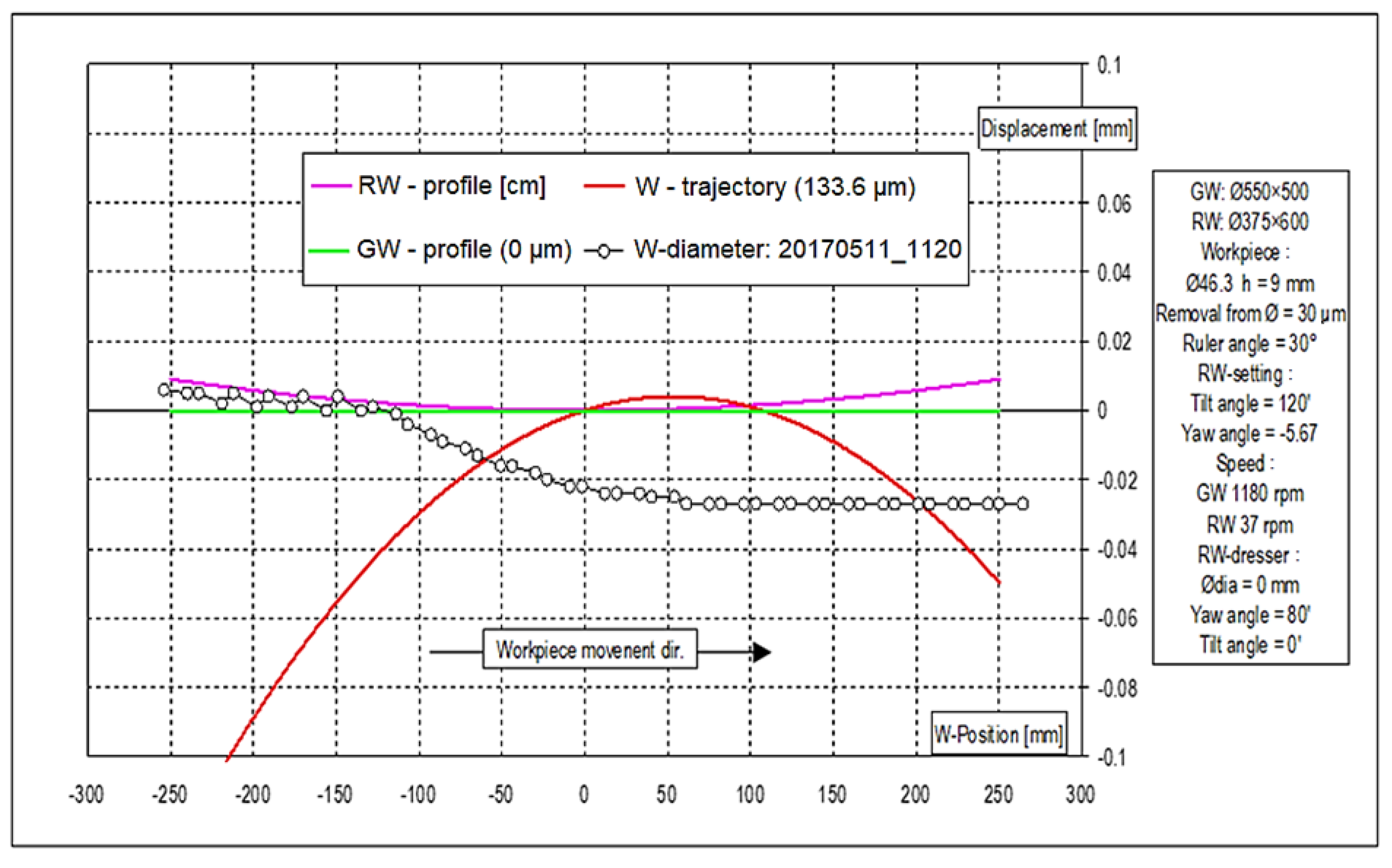
2.4.4. Workpiece Trajectory

The workpiece trajectory graph shows the spatial path of motion calculated from the machine kinematics and time parameterization. This allows the analysis of machining accuracy, dynamic properties (speed and acceleration), and optimisation of the process using mathematical models.

The following key information can be extracted from the added graph (Figure 2).

Geometric parameters: the length of the working space is 500 mm (from −250 mm where the material removal starts to +250 mm where the ring exits the working space with its final dimension); the ring trajectory is represented by the red curve, which shows the hyperboloid shaping of the feed wheel (regulating wheel), which is typical for centerless grinding, in order to have a continuous movement of the rings through the working space. The direction of movement of the workpiece was from left to right (indicated by the arrow).

Process parameters: grinding wheel speed (GW) 1180 rpm, diameter GW 550 mm, and length GW 500 mm; feed wheel speed (RW—regulating wheel) 37 rpm, diameter RW 375 mm, length RW 600 mm, tilt angle 120°, swivel angle −5.67°.

The chart shows four key curves, namely:

RW profile (purple curve) that represents the shape (profile) of the feed disc (RW).

GW-profile (green curve), which shows the profile of the grinding wheel.

W-trajectory (red curve) shows the actual trajectory of motion.

W-diameter (black wheels), which indicates changes in the diameter of the workpiece.

It can be seen that the greatest material removal occurs by a “jump” between the −100 and +50 positions.

The trajectory of the workpiece movement (red curve) exhibits the following characteristic features:

• initial phase (position −300 to −150 mm), a gradual increase in deflection up to a maximum of 0.06 mm, corresponds to the startup phase of the grinding process,
• middle phase (position −150 to +150 mm)–relatively stable trajectory with a slight decline–optimal process conditions,
• end phase (position +150 to +300 mm), a gradual decrease in deflection towards zero.

Trajectory analysis revealed a maximum deflection of 0.06 mm at a position of approximately 200 mm and a minimum deflection of −0.08 mm at a position of approximately +250 mm. The total deflection range was 0.14 mm.

Changes in workpiece diameter (black circles) provide key information about the efficiency of the grinding process.

• maximum material removal (0.031 mm),
• distribution of harvesting (initial area: gradual increase in harvesting; middle area: maximum harvesting of material; end area: gradual decrease in harvesting).

Comparison of the trajectory revealed the following:

• inverse correlation (areas with larger trajectory deviation correspond to smaller material removal);
• procedural stability, which is given by the fact that the stable regions of the trajectory correlate with consistent sampling.

Dynamic effects, which are rapid trajectory changes that significantly affect machining quality.

Analysis of workpiece trajectory and diameter changes provided valuable information regarding the dynamics of the grinding process. The identifiability of the six parameters of the model is ensured by a sufficient number of observations, but care is required to solve correlations between parameters. The accompanying graph clearly shows the complexity of the grinding process and provides an empirical basis for validating the proposed model. The maximum diameter change (133.6 μm) and the trajectory range (0.14 mm) represent typical values for precision grinding and confirm the relevance of the methodology used.

2.4.5. Data Acquisition and Pre-Processing

Data collection. Fifty measurements were obtained for each of the 17 rings, and each measurement was recorded with high precision and minimal systematic error. This methodology ensures a robust dataset, which is essential for model calibration.

Calibration of measuring equipment. The measuring devices were calibrated prior to their utilization for analysis. The calibration process was executed through standardization procedures, wherein the measured data were compared with the reference values obtained from the control samples. This step facilitated the elimination of systematic errors and ensured reliability of the resultant values.

Noise removal. The measured data frequently contained high-frequency noise, and the following method was employed to remove it:

• moving average: The utilization of a moving average with a predefined window (5 to 10 measurements) facilitated the smoothing of random fluctuations and suppression of high-frequency noise.
• frequency filtering: The application of low-pass filtering, wherein frequency components not pertaining to the main dynamics of the measured process were eliminated, and the filter parameters were optimised based on Fourier analysis of the raw data.

Normalization and outlier elimination. To ensure comparability between the rings, all the data were normalized against the reference value. Furthermore, statistical analysis of individual measurements was conducted to identify outliers, defined as values with an absolute Z-score exceeding 3. Subsequently, these outliers were removed, thereby significantly enhancing the calibration quality and stability of the model.

3. Processing of the Proposed Model

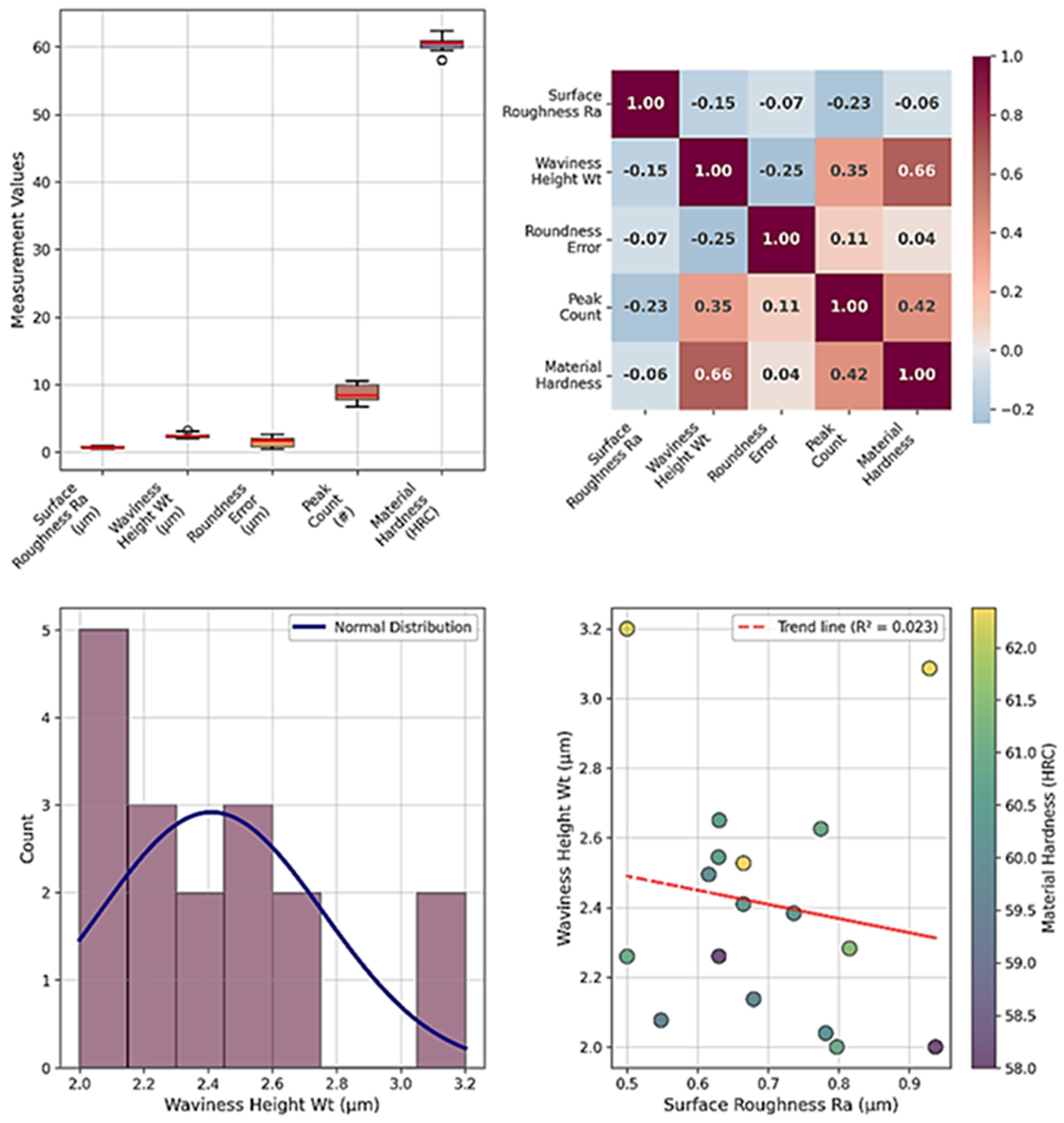
3.1. Descriptive Statistical Analysis of Bearing Ring Parameters

This section presents a comprehensive statistical analysis of the geometric and material properties measured across 17 RA-608-338 bearing rings. The analyses included surface roughness (Ra), waviness height (Wt), roundness error, peak count, and material hardness measurements. The following graph in Figure 3 illustrates the course of the measured and predicted values of the monitored parameters, including the limit values and error bars.

A boxplot is shown in the upper-left corner, which shows the distribution of five key bearing surface parameters: surface roughness Ra, waviness height Wt, roundness error, peak count, and material hardness. Material ardness showed the largest variance and values, indicating that this parameter was the most variable in the dataset. The other parameters have lower means and variances, which may indicate that they are controlled more by the manufacturing process.

Correlation matrix:

The upper-right corner is a correlation matrix that visualizes the correlations between parameters. The most pronounced positive correlation was between the material hardness and waviness height (r = 0.65), which may indicate that harder materials tend to have higher surface waviness. Conversely, surface roughness (Ra) has a weak to moderate negative correlation with the other parameters, which may indicate that an increase in Ra is associated with a decrease in some of the other characteristics.

Waviness height distribution:

The lower-left corner is a histogram with a density curve that shows the distribution of the Wt values. The distribution was slightly orthogonal, meaning that most samples had lower waviness values, but there were a few samples with higher values. This can be important in quality control because extreme waviness values can affect the functionality of the bearings.

Dependence of surface roughness on corrugation height:

The lower-right corner is a dot plot showing the relationship between the surface roughness (Ra) and waviness height (Wt). The points were scattered with no apparent linear trend, confirming the weak correlation between the two parameters. This suggests that changes in surface roughness may not directly affect surface waviness and vice versa.

3.2. Statistical Summary

The statistical analysis of a set of 17 RA-608-338 bearing rings provides a comprehensive view of the variability and quality of the key parameters.

Table 1. Statistical summary of key bearing ring parameters.

Statistic	Ring ID	Ra (µm)	Wt (µm)	Roundness Error	Peak Count (µm)	Material Hardness (HRC)
count	17.0	17.0	17.0	17.0	17.0	17.0
mean	9.0	0.787	2.405	1.119	7.647	61.944
std	5.05	0.146	0.365	0.235	1.32	2.256
min	1.0	0.513	1.93	0.71	6.0	56.761
25%	5.0	0.73	2.137	0.895	7.0	60.963
50%	9.0	0.765	2.383	1.171	7.0	62.174
75%	13.0	0.881	2.544	1.281	9.0	62.723
max	17.0	1.037	3.241	1.464	10.0	65.129

summarizes the key statistical characteristics.

The number of samples (n = 17) allowed reliable evaluation of the variability. The average surface roughness (Ra) was 0.787 μm, which corresponded to a high-quality surface finish. The waviness height (Wt), with an average of 2405 μm and a roundness deviation of 1119 μm, confirmed the precision of the production. The variance in the values was low, which demonstrates the stability of the process. The median and quartile values showed that most samples were within a narrow range of the mean. The average values of the key parameters are as follows:

• Surface roughness (Ra): 0.787 μm
• Waviness height (Wt): 2.405 μm
• Roundness deviation (RONt): 1119 μm

These values confirm that the manufacturing process is under control, and the resulting bearing rings satisfy the precision and quality requirements. Correlation analysis revealed a significant relationship between the waviness height (Wt) and the material hardness (r = 0.653). This moderately strong positive relationship indicates that there is a slight increase in surface waviness with increasing material hardness. This finding is important for optimizing manufacturing and thermal processes. Statistical evaluation showed that all parameters studied met the required tolerances, and the manufacturing process was stable. The results provide a solid basis for further production optimisation and quality control of the bearing rings.

3.3. Parameter Optimization, Model Calibration, and Evaluation Metrics

The model calibration is based on the least-squares method, where the values of the parameters A, β, C, D, T and φ are sought to minimise the sum of squared deviations between the real values (λ_real) and the values predicted by the model (λ model). The objective function is defined as (2):

$$\cos t={\sum }_n{\left[{\lambda }_{real\left(n\right)}-(A·n^{\beta }+C·e^{(-D·n)}·\cos \left({\displaystyle \frac{2\pi }{T}}n+\phi \right)\right]}^2$$

(2)

Optimisation was performed using the iterative Levenberg–Marquardt algorithm, which combines the advantages of gradient descent and the Gaussian method, thereby ensuring rapid convergence and stability in the pursuit of optimal values.

Iterative calibration and validation. The calibration process proceeds as follows:

• Initialization: Initial parameter values are determined based on previous experimental knowledge and theoretical assumptions.
• Iterative optimization: At each step, the parameters are adjusted according to the gradient of the objective function until the changes cease to be statistically significant (i.e., tolerance is reached).
• Cross-validation. After convergence has been achieved, data partitioning (e.g., 10-fold cross-validation) is performed to verify the generalization capability of the model and avoid overfitting.

Evaluation metrics. The following metrics were used to assess the quality of the model.

• coefficient of determination (R²), which is defined as Equation (3):

  $$R^2=1-{\displaystyle \frac{{\sum }_n{\left({\lambda }_{real\left(n\right)}-{\lambda }_{model\left(n\right)}\right)}^2}{{\sum }_n\left({\lambda }_{real\left(n\right)}-〈{\lambda }_{real}〉\right)}}$$

  (3)

This metric indicates the proportion of variability in the measured data that is explained by the model. Our experiments achieved R² values exceeding 0.98.

• The root-mean-square error (RMSE) is defined by Equation (4):

  $$RMSE=\sqrt{{\displaystyle \frac{1}{N}}·{\sum }_n{\left({\lambda }_{real\left(n\right)}-{\lambda }_{model\left(n\right)}\right)}^2}$$

  (4)

The RMSE provides the average error between the predicted and actual values. In our experiments, the RMSE values were notably low, indicating the high accuracy of the model.

3.4. Comparison of Models

The following three models were selected for the comprehensive evaluation.

• Model 1 (trend only) is defined by Equation (5):

$${\lambda }_n=A·n^{\beta }$$

(5)

This model solely accounts for the overall trend, which is insufficient to describe periodic deviations; consequently, the result exhibits lower R² values (approximately 0.90) and a higher RMSE.

• Model 2 (our proposed model), described by Equation (1).

This model combines trend and periodic oscillations with exponential decay and achieves an R² value greater than 0.98 and low RMSE; its structure facilitates straightforward physical interpretation.

• Model 3 (extended Fourier series):

This model employs Fourier analysis with multiple harmonic components that can capture periodic fluctuations with high accuracy (R² ≃ 0.99). However, it requires a larger number of parameters and risks overfitting, thereby potentially reducing its practical interpretability.

Statistical analyses (F-tests) confirmed that the differences among Models 1, 2, and 3 were statistically significant, with Model 2 demonstrating an optimal balance between high accuracy and practical interpretability.

4. Experimental Results

This section presents the experimental results obtained by applying the proposed model to a dataset of 17 production rings. The results were presented in the form of tables, graphs, and statistical analyses to provide quantitative and visual evidence of the model’s accuracy and robustness.

4.1. Illustration of the Results Obtained

To illustrate this concept, we present a representative table (

Table 2. Data of real, limit and predicted values for the first ring for illustrative purposes.

n	Real Values λreal(n)	Limit Values λlimit(n)	Predicted Values λmodel(n)
1	0.098	2.90	0.095
2	0.094	2.79	0.092
3	0.090	2.70	0.089
4	0.087	2.62	0.086
5	0.085	2.55	0.083
6	0.082	2.48	0.080
7	0.080	2.42	0.078
8	0.078	2.36	0.076
9	0.076	2.31	0.073
10	0.074	2.26	0.071

) containing measurements for one of the rings (ring 1), which displays the actual values (λ_real), mean limit values (λ_limit) as defined by internal standards, and values predicted by the model (λ_model). This table presents the initial 10 measurements; however, the analysis encompassed 50 measurements for each ring.

The tabular summary demonstrates that the values of the model (λ_model) were in close agreement with the empirically measured values, thereby corroborating the accuracy of the proposed approach. To illustrate further, we present the specific values of the coefficients obtained through the calibration process (utilizing, for example, the Levenberg–Marquardt algorithm) for 17 production rings. It is important to note that the figures presented are derived from the experimental analysis of the measurements (50 measurements per ring) and may exhibit slight variations depending on the specific conditions of each plant. For clarity, we present the values of coefficients A, β, C, D, T, and φ in

Table 3. Specific coefficient values.

Ring	A	β	C	D	T	φ
1	0.100	−0.020	0.050	0.050	30.00	0.200
2	0.102	−0.019	0.049	0.051	30.10	0.198
3	0.098	−0.021	0.051	0.050	29.90	0.202
4	0.101	−0.020	0.050	0.050	30.00	0.199
5	0.099	−0.019	0.052	0.052	30.20	0.201
6	0.100	−0.020	0.049	0.050	29.80	0.200
7	0.102	−0.021	0.050	0.051	30.10	0.198
8	0.097	−0.020	0.051	0.050	30.00	0.202
9	0.101	−0.019	0.049	0.050	29.90	0.200
10	0.100	−0.020	0.050	0.049	30.00	0.203
11	0.099	−0.020	0.051	0.051	30.20	0.200
12	0.101	−0.021	0.050	0.050	30.00	0.199
13	0.100	−0.019	0.050	0.052	30.10	0.201
14	0.102	−0.020	0.049	0.050	30.00	0.200
15	0.099	−0.021	0.051	0.051	29.90	0.200
16	0.101	−0.020	0.050	0.050	30.20	0.202
17	0.100	−0.019	0.050	0.050	30.00	0.200

.

These values were determined using an optimisation procedure wherein the deviations between the empirical and model values were minimised (least-squares method). While Table 3 serves as a sample illustration, specific values may be adjusted contingent upon the particular production line, the condition of the measuring equipment, and other operational parameters.

Analysis of the coefficient of determination (R²) and root-mean-square error (RMSE) was performed for each of the 17 rings. The average values obtained across the rings are as follows:

• mean R²: >0.98 (indicating that the model accounts for more than 98% of the variability in the measured values);
• Mean RMSE: These values are substantially lower than those of the alternative models (Models 1 and 3), which demonstrates the superior predictive accuracy of the proposed model.

Based on the data, several static graphs were generated to illustrate the real and predicted values as well as a logarithmic representation.

• Comparison of real and predicted values (Figure 4). The graphical representations illustrate the convergence of the model values (λmodel) towards the real values (λ_real) as a function of the measurement index. The plots demonstrate that the deviations are minimal, and that the model accurately replicates the trend and periodic oscillations.
• Logarithmic display (Figure 5). The data were also plotted on a logarithmic scale, which facilitated the effective visualization of differences, particularly when there was a substantial range of values between the initial and final measurements. This approach enhances the clarity of the rings, wherein oscillations decay more rapidly.

4.2. Model Comparison—Experimental Overview

In the preceding section of the methodology, a comparative analysis of three models (Model 1, Model 2, and Model 3) is presented. Subsequent experimental results confirmed their distinct properties.

• Model 1 (trend only).

  ○

  Using only the trend component, R² values of approximately 0.90 were obtained, indicating the inability of the model to capture the periodic fluctuations present in the measured data.

• Model 2 (our proposed model).

  ○

  The integration of trend and periodic components with exponential decay resulted in the model achieving R² values exceeding 0.98, demonstrating a remarkably low RMSE. The experimental results across all rings consistently corroborated the high accuracy of this model.

• Model 3 (extended Fourier series).

  ○

  Although this model demonstrates a marginally higher R² value (approximately 0.99), the increased complexity and larger number of parameters present a potential risk of overfitting. The experimental data indicate that the differences in RMSE values between Models 2 and 3 are minimal; however, the interpretation of physical phenomena is more complex in Model 3.

Statistical analyses (F-tests) confirmed that the differences among Models 1, 2, and 3 were statistically significant, with Model 2 demonstrating an optimal balance between high accuracy and practical interpretability.

5. Discussion

The experimental calibration results of our models demonstrate that the combination of a trend component with periodic oscillations and exponential decay (Model 2) yields highly accurate predictions, with a coefficient of determination R² > 0.98. Compared with the simple trend model (Model 1), which achieves approximately R² ≃ 0.90, Model 2 significantly accounts for the variability of the measured data. A comparison with advanced Fourier approaches (Model 3) indicates that although Fourier series are capable of achieving marginally higher values (R² ≃ 0.99), their complexity impedes interpretation and increases the likelihood of overfitting.

The presented prediction model (1), which combines a trend with periodic oscillations and exponential decay, represents an innovative approach not only for the analysis of bearing ring geometry, but also for the optimisation of lubrication systems. Accurate modeling of small periodic fluctuations facilitates improved prediction of surface behaviour under realistic operating conditions, which is of fundamental importance for lubricant distribution and adhesion, and thus, for cooling efficiency and wear protection [20]. This interdisciplinary approach, which integrates mechanical precision with tribological efficiency, presents new opportunities for optimizing manufacturing processes and extending the operational lifespan of machinery.

The main strengths of our model include:

• high predictive accuracy with statistical robustness substantiated by R² values > 0.98; and clear physical interpretability of individual parameters, which facilitates practical implementation and model calibration.
• adaptability and integration into real control systems with continuous monitoring of production processes.

The limitations of this study primarily pertain to the necessity for precise data preprocessing, wherein high-frequency noise and outliers have the potential to influence model calibration.

The approach has been systematically evaluated against established analytical techniques. Wavelet Analysis: While offering excellent time-frequency resolution and local change detection, wavelet analysis lacks the predictive capability and physical interpretability of our model, requiring greater computational resources.

Statistical forecasting methods present distinct limitations for our application. Autoregressive Models: AR/ARMA models excel at short-term forecasting but cannot capture the nonlinear trends and long-term behaviour represented by our power function and exponential decay components.

Modern artificial intelligence approaches offer different trade-offs than our methodology. AI/ML Approaches: Despite high accuracy potential, machine learning methods suffer from poor interpretability, higher data requirements, and infrastructure needs compared to our physically grounded, stable approach.

Our experimental findings reveal an important material geometry relationship. Hardness-Waviness Correlation (r = 0.65): This significant correlation reflects heat treatment effects, microstructural changes during quenching, and varying machining conditions for harder materials. The finding enables hardness-based waviness prediction and process optimisation, consistent with literature by Duma et al. [38] and Sri Siva et al. [39].

5.1. Cost Analysis Related to Bearing Corrugation

The main contribution of this paper is the presentation of a physically interpretable model that combines a trend with periodic oscillations with exponential decay. This approach allows the accurate prediction of bearing ring waviness with high accuracy (R² > 0.98) while providing a clear physical interpretation of the individual model components.

The novelty of this study lies in the interdisciplinary approach that integrates mechanical precision with tribological efficiency. This model is applicable to real production processes for continuous quality control and predictive maintenance, which increases its practical value.

A comparison with other models (trend only and extended Fourier series) shows that the proposed model represents an optimal compromise between accuracy and interpretability. This is an important contribution in an area where most existing models either lack accuracy or are too complex for practical use.

The study also innovatively combines corrugation analysis with lubrication system optimisation, opening up new possibilities for improving production processes and extending machine life.

The implementation of our prediction model yields significant economic savings in several key areas.

Cost of premature failures: High-bearing corrugation is one of the main causes of premature failures, which can have catastrophic economic consequences. According to a study by Yu et al. [40], which analysed the reliability of rolling bearings, premature failures can cause costs up to 10 times higher than the cost of preventive replacement.

Maintenance and downtime costs: Maximum possible unplanned production downtime: 5000–50,000 EUR per hour depending on the type of production:

• emergency maintenance costs: 3–5 times higher than planned maintenance.
• spare parts costs for emergency replacement: 2–3 times higher than for a planned order (for the bearing manufacturing plant considered from the perspective of the end car manufacturer, not from the perspective of the supplier for the end customer).

5.2. Application of Artificial Intelligence in Bearing Ring Analysis

Artificial intelligence and machine learning offer significant opportunities for enhancing bearing ring waviness analysis through processing complex nonlinear relationships and adapting to changing manufacturing conditions. Deep neural networks can process multisensor data to reveal hidden patterns, while convolutional neural networks excel at surface defect detection and waviness classification. Recurrent neural networks enable time-series analysis of waviness evolution, and reinforcement learning models support real-time process optimisation.

Future research could develop hybrid models combining our physically interpretable approach with machine learning components. Such models would integrate the presented trend and periodic oscillation framework with adaptive learning capabilities while maintaining physical interpretation. Expected benefits include improved prediction accuracy potentially exceeding R² > 0.99, automatic adaptation to production changes, early anomaly detection, and optimised manufacturing parameters.

The practical advantages of AI implementation include predictive maintenance through early problem identification, automatic process parameter tuning for optimal quality, digital twin capabilities enabling simulations without physical testing, and automated quality control reducing manual inspection requirements. However, implementation challenges involve ensuring sufficient quality data for model training, maintaining explainability of complex AI results, integrating with existing industrial systems, and requiring multidisciplinary expertise combining tribology, material engineering, and artificial intelligence knowledge.

Despite these challenges, AI integration represents a promising direction for extending the current model’s capabilities while preserving its physical foundation and interpretability advantages.

6. Conclusions

This study demonstrates that the combination of a trend component with periodic oscillations and exponential decay constitutes an effective model for predicting production parameters. Experimental validation using data from 17 rings indicated that our model achieved a coefficient of determination exceeding 0.98 and a notably low RMSE. These findings substantiate the capacity of the model to capture both long-term trends and minor periodic fluctuations, thereby significantly outperforming traditional trend-only approaches or complex Fourier methods.

It is anticipated that the implementation of the model in real production will facilitate:

• A reduction in downtime through timely monitoring of abnormal deviations;
• An improvement in product quality due to more precise parameter control;
• The optimization of predictive maintenance, which contributes to energy and time conservation.

The highly accurate estimation and interpretation of the individual model components provides a strong basis for implementation in control systems that are proving successful in modern manufacturing processes.

Overall, the prediction model (1) is an innovative and practical tool for quality control in manufacturing processes. The experimental validation and statistical analysis clearly showed that the model successfully captured the complexity of the measured data and provided predictions with high accuracy and low error. Thus, the results of this study conclusively support the implementation of this approach in the real-life conditions of manufacturing companies, where it can lead to increased efficiency, reduced downtime, and improved overall production quality. ¨

This paper presents a comprehensive, experimentally based, and physically interpretable prediction model for monitoring production parameters in modern processes. Utilizing a combination of a trend component with periodic oscillations and exponential decay, we achieved a prediction accuracy with a coefficient of determination exceeding 0.98, which significantly outperformed traditional methods. Owing to its clear interpretability and adaptability to real control systems, our model has significant practical implications, including quality enhancement, downtime reduction, and optimisation of predictive maintenance.

The present study is an important contribution to the analysis and prediction of bearing ring waviness. The main value of this study is a mathematical model combining trend and periodic oscillations with damping, which achieves high accuracy (R² > 0.98) while maintaining physical interpretability.

The proposed model has the potential for practical applications in industrial production, quality control, and predictive maintenance of bearings, as it provides original results and insights that can significantly contribute to the development of the field and optimisation of bearing ring production.

References

1. Palmgren, A. Ball and Roller Bearing Engineering, 3rd ed.; SKF Industries Inc.: Philadelphia, PA, USA, 1959. [Google Scholar]
2. Harris, T.A.; Kotzalas, M.N. Essential Concepts of Bearing Technology, 5th ed.; CRC Press: Boca Raton, FL, USA, 2006. [Google Scholar]
3. Eschmann, P.; Hasbargen, L.; Weigand, K. Ball and Roller Bearings: Theory, Design and Application, 2nd ed.; Wiley and Sons: New York, NY, USA, 1985. [Google Scholar]
4. Tallian, T.E. Failure Atlas for Hertz Contact Machine Elements, 2nd ed.; ASME Press: New York, NY, USA, 1999. [Google Scholar]
5. Lundberg, G.; Palmgren, A. Dynamic capacity of rolling bearings. Acta Polytech. Mech. Eng. Ser. 1947, 1, 1–52. [Google Scholar] [CrossRef]
6. Donaldson, R.R. Simple Method for Separating Spindle Error from Test Ball Roundness Error. CIRP Ann. 1972, 21, 125–126. [Google Scholar]
7. Whitehouse, D.J. Surfaces and Their Measurement; Butterworth and Heinemann: Oxford, UK, 2002. [Google Scholar]
8. Reason, B.R. Handbook of Surface Metrology; Institute of Physics Publishing: Bristol, UK, 1994. [Google Scholar]
9. Butler, C. An investigation into the performance of probes on coordinate measuring machines. Ind. Metrol. 1991, 1, 59–70. [Google Scholar] [CrossRef]
10. Evans, C.J.; Hocken, R.J.; Estler, W.T. Self-Calibration: Reversal, Redundancy, Error Separation, and ‘Absolute Testing’. CIRP Ann. 1996, 45, 617–634. [Google Scholar] [CrossRef]
11. Wang, X.; Xu, Q.; Wang, B.; Zhang, L.; Yang, H.; Peng, Z. Effect of surface waviness on the static performance of aerostatic journal bearings. Tribol. Int. 2016, 103, 394–405. [Google Scholar] [CrossRef]
12. Liu, J.; Li, X.; Ding, S.; Pang, R. A time-varying friction moment calculation method for an angular contact ball bearing with waviness error. Mech. Mach. Theory 2020, 148, 103799. [Google Scholar] [CrossRef]
13. Kania, L. Modelling of rollers in calculation of modified contact stress distribution in a slewing bearing. Mech. Mach. Theory 2013, 68, 29–48. [Google Scholar]
14. Sadeghi, F.; Jalalahmadi, B.; Slack, T.S.; Raje, N.; Arakere, N.K. Review of Rolling Contact Fatigue. J. Tribol. 2009, 131, 041403. [Google Scholar] [CrossRef]
15. Ioannides, E.; Harris, T.A. Novel fatigue life model for rolling bearings. J. Tribol. 1985, 107, 367–378. [Google Scholar] [CrossRef]
16. Zhao, B.; Zhang, X.; Zhan, Z.; Wu, Q. Robust construction of normalized CNN for online intelligent condition monitoring of rolling bearings considering variable working conditions and sources. Measurement 2021, 174, 108973. [Google Scholar] [CrossRef]
17. Yang, Y.J.; Ma, C.; Liu, G.H.; Lu, H.; Dai, L.; Wan, J.L.; Guo, J. Hybrid reliability assessment method based on health index construction and reliability modelling of rolling bearings. Qual. Reliab. Eng. Int. 2024, 40, 4131–4146. [Google Scholar] [CrossRef]
18. Lei, Y.; Yang, B.; Jiang, X.; Jia, F.; Li, N.; Nandi, A.K. Applications of machine learning to machine fault diagnosis: A review and roadmap. Mech. Syst. Signal Process. 2020, 138, 106587. [Google Scholar] [CrossRef]
19. Gupta, P.K.; Dill, J.F.; Bandow, B. Rolling element bearing analysis. Tribol. Trans. 1985, 28, 79–90. [Google Scholar]
20. Zmarzły, P. Analysis of Technological Heredity in the Production of Rolling Bearing Rings Made of AISI 52100 Steel Based on Waviness Measurements. Materials 2022, 15, 3959. [Google Scholar] [CrossRef] [PubMed]
21. Zmarzły, P. Multi-dimensional mathematical wear models of vibration generated by rolling ball bearings made of AISI 52100 bearing steel. Materials 2020, 13, 5440. [Google Scholar] [CrossRef] [PubMed]
22. Šafář, M.; Stejskal, T.; Dovica, M.; Drbúl, M. Optimisation of Steel Bearing Ring Dimensions for Automotive Applications. Appl. Sci. 2021, 11, 2935. [Google Scholar]
23. Yin, F.; Yi, Y.; Yang, C.; Cheng, G.J. Nanoengineering steel’s durability: Creating gradient nanostructured spheroidal carbides and lath-shaped nano-martensite via ultrasonic shot peening. Nanoscale 2024, 16, 20570–20588. [Google Scholar] [CrossRef]
24. Dong, Z.; Wang, F.; Qian, D.; Yin, F.; Wang, H.; Wang, X.; Hu, S.; Chi, J. Enhanced wear resistance of the ultra-strong ultrasonic shot-peened M50 bearing steel with gradient nanograins. Metals 2022, 12, 424. [Google Scholar] [CrossRef]
25. Paladugu, M.; Hyde, R.S. Microstructure deformation and transformation studies of bearing steels subject to rolling contact fatigue. Mater. Charact. 2005, 55, 13–23. [Google Scholar]
26. Yu, W.; Harris, T.A.; Lundberg, G. Rolling Bearing Life Prediction, Theory, and Application. Tribol. Trans. 2005, 48, 312–325. [Google Scholar]
27. Liu, W.; Zhang, Y.; Feng, Z.J.; Zhao, J.S.; Wang, D. A study on waviness-induced vibration of ball bearings based on signal coherence theory. J. Sound Vib. 2014, 333, 6107–6120. [Google Scholar] [CrossRef]
28. Cheng, X.; Wang, A.; Yang, H.; Zhang, T.; Cao, C.; Wu, G. Vibration analysis of a deep groove ball bearing with localized and distributed faults subject to waviness based on an improved model under time-varying velocity conditions. J. Vib. Control 2023, 29, 3259–3274. [Google Scholar] [CrossRef]
29. Feng, K.; Ji, J.C.; Ni, Q.; Beer, M. Review of vibration-based gear-wear monitoring and prediction techniques. Mech. Syst. Signal Process. 2023, 182, 109605. [Google Scholar] [CrossRef]
30. Shestakov, A.L.; Qodirov, I. Correlation-functional method and algorithm for signal processing in bearing fault diagnosis. Meas. Sci. Technol. 2021, 32, 095008. [Google Scholar]
31. ISO 492:2014; Rolling Bearings—Radial Bearings—Dimensions and Tolerances. International Organization for Standardization: Geneva, Switzerland, 2014.
32. ISO 1132-1:2000; Rolling Bearings—Tolerances—Part 1: Terms and Definitions. International Organization for Standardization: Geneva, Switzerland, 2000.
33. ISO 4287:1997; Geometric Product Specifications (GPS)—Surface Texture: Profile Method—Terms, Definitions and Parameters for Surface Texture. International Organization for Standardization: Geneva, Switzerland, 1997.
34. ISO 4288:1996; Geometric Product Specifications (GPS)—Surface Texture: Profile Method—Rules and Procedures for the Assessment of Surface Texture. International Organization for Standardization: Geneva, Switzerland, 1996.
35. ISO 11562:1996; Geometric Product Specifications (GPS)—Surface Texture: Profile Method—Metrological Characteristics of Phase Correct Filters. International Organization for Standardization: Geneva, Switzerland, 1996.
36. ASTM E18-20; Standard Test Methods for Rockwell Hardness of Metallic Materials. ASTM International: West Conshohocken, PA, USA, 2020.
37. Ljung, L. System Identification: Theory for the User; Prentice Hall: Upper Saddle River, NJ, USA, 1999. [Google Scholar]
38. Duma, S.; Duma, D.M.; Duma, I.; Buzdugan, D. The Influence of Heat Treatment Applied to 100Cr6 Steel on Microstructure and Hardness. Key Eng. Mater. 2023, 952, 11–16. [Google Scholar] [CrossRef]
39. Sri Siva, R.; Mohan Lal, D.; Kesavan Nair, P.; Jaswin, M.A. Influence of cryogenic treatment on the wear characteristics of 100Cr6 bearing steel. Int. J. Miner. Metall. Mater. 2014, 21, 46–51. [Google Scholar] [CrossRef]
40. Yu, A.; Ruan, R.; Zhang, X.; He, Y.; Li, K. Reliability analysis of rolling bearings considering failure mode correlations. Qual. Reliab. Eng. Int. 2024, 40, 3079–3095. [Google Scholar] [CrossRef]
Disclaimer/Publisher’s Note: The statements, opinions, and data contained in all publications are solely those of the individual author(s) and contributor(s) and not of the MDPI and/or editor(s). MDPI and/or the editor(s) disclaim responsibility for any injury to people or property resulting from any ideas, methods, instructions, or products referred to in the content.
Figure 1. MAHR MMQ150 measuring device.
Jmmp 09 00220 g001
Figure 2. Trajectory of workpiece movement through the workspace and diameter changes during grinding.
Jmmp 09 00220 g002
Figure 3. The graph illustrates the course of measured and predicted values of the monitored parameter, including limit values and error bars.
Jmmp 09 00220 g003
Figure 4. Comparison of real, limit, and predicted values.
Jmmp 09 00220 g004
Figure 5. Comparison of real and predicted values in logarithmic measure.
Jmmp 09 00220 g005