New Hybrid Method for Buffer Positioning and Production Control Using DDMRP Logic in Smart Manufacturing

Abstract

Despite its proven effectiveness in inventory management across various industries, Demand-Driven Material Requirements Planning (DDMRP) remains largely a manual process, with few studies investigating its numerical integration. This research proposes a novel multi-stage production control framework grounded in DDMRP principles, enabling effective scheduling of production orders based on either demand forecasts or actual demand, when available. A mixed-integer programming (MIP) model is developed to capture the dynamic interactions between demand, buffer positioning, and replenishment policies, supporting reactive production planning in smart, reconfigurable manufacturing environments. To identify the optimal buffer locations, a Genetic Algorithm (GA) is employed. The MIP model provides the GA with production planning outputs used to evaluate the fitness of decisions regarding buffer placement. To demonstrate the effectiveness of this hybrid GA–MIP approach, simulations are conducted on three representative production configurations. The results show that the proposed method significantly improves the theoretical performance of each configuration by determining optimal buffer locations and planning replenishments, achieving a better balance between inventory levels and demand fulfillment.

1. Introduction

In modern manufacturing systems, production inventories play an essential role in maintaining workflow continuity, mitigating variability, and optimizing system performance. The strategic allocation and distribution of buffers are critical for addressing operational challenges such as bottlenecks, downtime, and production variability. Effective buffer allocation and management is addressed by implementing an appropriate Production Planning and Control (PPC) system, whether pull or push based.

Demand-Driven Material Requirements Planning (DDMRP) is a PPC methodology introduced by [1]. It is described as a hybrid push–pull strategy that integrates real-time stock and customer demand observations (pull) with anticipatory demand forecasting (push). DDMRP has demonstrated superior competitiveness compared to traditional PPC systems such as Kanban, Materials Requirements Planning (MRP), and Optimized Production Technology (OPT) [2]. The method has been successfully implemented across various industries, with notable examples including CCBA (Coca Cola bottling partner), Shell, ArcelorMittal Brazil, FORGE USA, NLMK, Legrand, and Michelin [3].

DDMRP is grounded in a bimodal inventory distribution model that defines two critical boundaries: the stock shortage and stock excess points. The method determines these levels using demand forecasting and supply chain Lead Times while maintaining continuous stock level control through demand-driven replenishment orders. A key feature of DDMRP is its use of “decoupling/isolation points”, which are strategic buffers used to mitigate the impact of variability on material flow throughout the supply as shown in Figure 1:

The Decoupled Lead Time (DLT) refers to the time required to supply the next production unit with input materials. It is termed “decoupled” because it results from the introduction of a buffer, which breaks the direct dependency between supply and demand. In DDMRP, each buffer is divided into three zones, conventionally identified by colors: Top of Green (TOG), Top of Yellow (TOY), and Top of Red (TOR).

TOR can be seen as safety stock limit used to protect against shortages. TOY is a stock layer that is used to respond to demands that cannot be satisfied using replenishment due to Lead Time delay. Finally, TOG is an extra protection that takes into consideration eventual supply chain fluctuations that impact Decoupled Lead Time (DLT). Calculation of these levels are detailed in Section 3.

According to [4], the core concepts of DDMRP include the following:

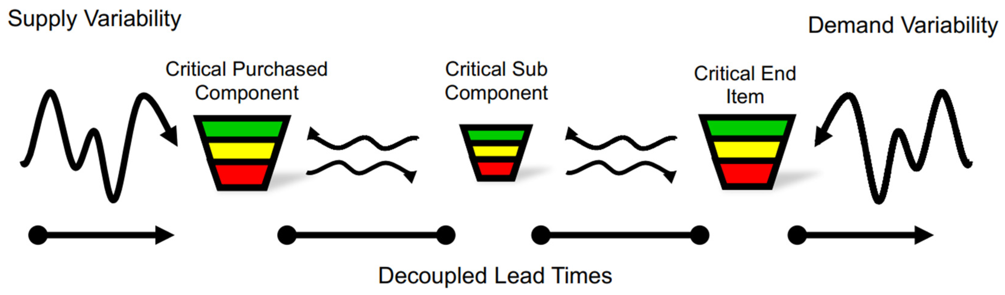
• Strategic Inventory Positioning: Identifying critical points within the supply chain for buffer placement, which act as decoupling points to absorb variability and protect material flow.
• Buffer Profiles and Levels: Establishing buffer zones (green, yellow, red) at these critical points, dynamically adjusted based on Lead Times, Demand Variability, and supply reliability.
• Dynamic and Reactive Adjustments: Continuously refining buffer levels in response to changes in demand patterns and supply conditions to optimize inventory levels.
• Demand-Driven Planning: Utilizing actual demand data to drive replenishment decisions, reducing reliance on forecasts, and minimizing the bullwhip effect.
• Visible and Collaborative Execution: Ensuring real-time supply chain visibility and fostering collaboration to promptly address issues and align actions with current market conditions.

Although an extensive body of literature exists on DDMRP concepts—as detailed in the following section—relatively few studies have proposed fully automated methods that implement all DDMRP steps, from buffer placement to production planning within a defined planning horizon. Recent research has introduced hybrid approaches that integrate DDMRP with optimization techniques, aiming to address specific aspects such as parameterization, buffer positioning, or production scheduling.

The main contribution of this article is the proposal of a systematic and reactive approach to simultaneously determine optimal buffers placement and perform production control within a planning horizon for configurable multi-stage production systems. Accordingly, Section 2 reviews the current state of the art in DDMRP research. Section 3 introduces a mixed-integer programming model for Production Planning and Control based on DDMRP principles. Section 4 describes the Genetic Algorithm used to optimize buffer positioning based on the outputs of production control model used as prediction tool. Section 5 presents a case study, and the final section offers conclusions and directions for future research.

2. State of the Art

Compared to well-established Production Planning and Control systems such as MRP and Kanban, the body of literature on Demand-Driven Material Requirements Planning remains relatively sparse. Nevertheless, the method has garnered significant attention from the research and industrial communities, many of whom believe it represents the future of production planning [5,6].

Introduced a decade ago by [1], approximately 20 research articles addressing DDMRP have been published over the past 10 years. These contributions can be categorized into four primary domains:

• Conceptual Studies and Literature Reviews: This group includes seminal works such as the foundational books by [1,7], which established the theoretical underpinnings of DDMRP by integrating concepts from MRP, Kanban, and other planning methods. Literature reviews in this category aim to define the key principles and applications of DDMRP, situating it within the broader landscape of production planning.
• Comparative and Case Studies: Studies in this domain assess DDMRP’s performance relative to traditional PPC systems. These comparisons, often conducted through statistical analyses or simulation models, consistently demonstrate DDMRP’s superiority in terms of service level and operational costs [8,9,10]. For instance, [2] found that DDMRP outperforms other PPCs in regards of bottlenecks, demand variability, and Due Date Tightness.
• Buffer Positioning: Buffer positioning—the first step in DDMRP implementation—involves determining which items in the Bill of Materials should be protected by buffers. This decision is critical, as buffer stocks incur operational costs and should be applied selectively to high-risk items that are vulnerable to demand variability. Research in this area includes optimization-based approaches for strategically positioning buffers. For example, [11] proposed a Genetic Algorithm to optimize buffer placement by balancing operational costs and service levels in a single-stage production setting. Similarly, [12] introduced a mixed-integer programming model for buffer positioning aimed at minimizing buffer levels. However, the first approach provides no performance guarantees, while the second relies on average stock estimates without accounting for actual replenishment triggers.
• Parameterization of DDMRP: Once buffers are positioned, their sizing and replenishment parameters must be determined. These parameters, such as Lead Time Factor and Variability Factor, are often fixed subjectively. [13] suggest using statistical analysis to derive parametrization rules. Some other papers, namely [14], suggest automatic procedures driven by optimization to fix the parameters of DDMRP. In [11], a multi-objective metaheuristic to parameterize DDMRP is proposed. The method determines a comprehensive set of eight parameters while maximizing On Time Demand and minimizing average stock for one production unit. The method combines simulation and optimization [15] to yield solutions rapidly. However, the solutions come with no performance guarantee, which constitutes the major drawback of the method.

Considering the current state of the art, buffer positioning and production control in DDMRP remain open challenges—particularly when addressing the complexity of real-world applications through complete, multi-stage approaches. Moreover, recent studies have highlighted the potential of integrating DDMRP with emerging Industry 4.0 technologies [16,17]. The incorporation of real-time data analytics and IoT-based systems can significantly enhance DDMRP’s responsiveness to variability. Such integration supports the development of reconfigurable systems, aligning with DDMRP.

Consequently, this article proposes a broader integration of DDMRP as an automated approach for simultaneously optimizing buffer positioning and managing order replenishments within a planning horizon in multi-stage production systems. The proposed method is designed to be compatible with Industry 4.0 technologies, enabling its deployment in reconfigurable manufacturing environments. The following sections present the mathematical formulation of the problem as a mixed-integer programming model, followed by its integration with a Genetic Algorithm.

3. Problem Statement and Mathematical Modeling of DDMRP

The implementation of DDMRP begins with the positioning of buffers, which serve as decoupling points within the supply chain. These buffers enhance supply chain agility and effectively mitigate the bullwhip effect. According to the Association for Supply Chain Management [18], decoupling is defined as: Creating independence between supply and use of material. Commonly denotes providing inventory between operations so that fluctuations in the production rate of the supplying operation do not constrain production or use rates of the next operation.

Consequently, the initial step in DDMRP involves placing buffers between production stations. Indiscriminately adding a buffer after every station is suboptimal due to the associated inventory holding costs. The primary objective is to optimize buffer placement and sizing to balance inventory costs with system responsiveness. In the short term, the system must dynamically adjust buffer levels based on customer demand evolution, ensuring timely replenishment to prevent production bottlenecks. The overarching goal is to develop an autonomous and configurable system capable of automatic buffer activation. Figure 2 demonstrates a typical integration of PPC system leveraging DDMRP principles.

The Production Planning and Control (PPC) system as a Level 3 control component interfaces with or will be embedded within the Manufacturing Execution System. Using the Advanced Message Queuing Protocol [19]—typically adopted in modern production control systems—PPC monitors buffer levels in real time and triggers replenishments when inventory falls below reorder points. Additionally, the PPC system interacts with Enterprise Resource Planning systems to access real-time customer demand data.

If necessary, the system autonomously activates buffers and plans future replenishments to improve service levels by reducing Decoupled Lead Time and increasing robustness against demand fluctuations. This is based on the model below and considers the following characteristics, along with the production configuration illustrated in Figure 3:

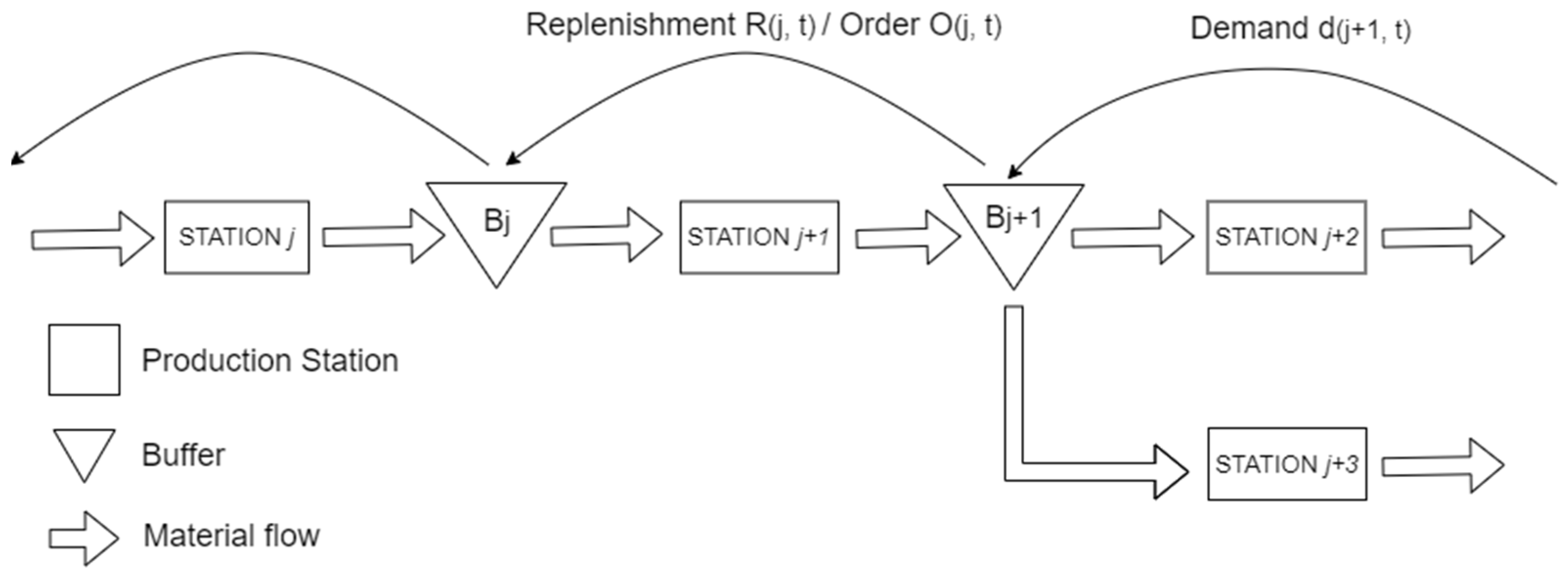
• The system consists of J production stations arranged in a topology with diverging branches, designed to accommodate the processing of multiple product references.
• The processing time p_j at each station j is assumed to be constant.
• The primary source of variability is the incoming demand, which directly affects the output stations.
• Each output station is associated with a specific product reference; thus, the model addresses multi-reference Production Planning and Control.
• The production flow is constrained to a directed acyclic structure.
• Only production systems for manufactured products with internal supply chains are considered. This assumption influences the estimation of lead time variations, which will be explicitly modeled in the analysis.

By considering a planification horizon H, the primary decision metric used in DDMRP to trigger replenishment is the Net Flow, denoted by ${\mathrm{N}}_{\mathrm{j},\mathrm{t}}^{\mathrm{f}\mathrm{l}\mathrm{o}\mathrm{w}}$ and defined by Equation (1):

$${\mathrm{N}}_{\mathrm{j},\mathrm{t}}^{\mathrm{f}\mathrm{l}\mathrm{o}\mathrm{w}}={\mathrm{x}}_{\mathrm{j}}.{\mathrm{B}}_{\mathrm{j},\mathrm{t}}+{\mathrm{I}}_{\mathrm{j},\mathrm{t}}-{\tilde{\mathrm{d}}}_{\mathrm{j},\mathrm{t}}\hspace{1em}\forall \mathrm{j} ϵ \mathrm{J},\forall \mathrm{t} ϵ \mathrm{H}$$

(1)

Net Flow indicates the balance between supply and demand at a specific buffer called on-hand inventory designated by ${\mathrm{B}}_{\mathrm{j},\mathrm{t}}$. It represents the stock physically available at a station j at a given instant t. When ${\mathrm{N}}_{\mathrm{j},\mathrm{t}}^{\mathrm{f}\mathrm{l}\mathrm{o}\mathrm{w}}$ is under a certain threshold, replenishment orders are triggered. ${\mathrm{I}}_{\mathrm{j},\mathrm{t}}$ designates on-order inventory and refers to the confirmed incoming supplies, such as purchase orders, manufacturing orders, or transfer orders that are expected to replenish the buffer. The main decision variable in the model is ${\mathrm{x}}_{\mathrm{j}}$ and indicates if the station j contains a buffer or not:

$${\mathrm{x}}_{\mathrm{j}}=\left\{\begin{array}{c}1 \mathrm{if} \mathrm{the} \mathrm{station} \mathrm{j} \mathrm{has} \mathrm{a} \mathrm{buffer}\hfill \\ 0 \mathrm{Otherwise}\hfill \end{array}\right. \forall \mathrm{j} ϵ \mathrm{J}$$

(2)

${\tilde{\mathrm{d}}}_{\mathrm{j},\mathrm{t}}$ refers to the qualified demand, involving confirmed customer orders or forecasts over a defined horizon. Qualified demand is adaptation of the real demand on station j to take in consideration any future peak of demand as given by Equation (3):

$${\tilde{\mathrm{d}}}_{\mathrm{j},\mathrm{t}}={\mathrm{d}}_{\mathrm{j},\mathrm{t}}+\sum _{{\mathrm{t}}^{\prime }=\mathrm{t}}^{\mathrm{t}+\mathrm{P}\mathrm{H}}{\mathrm{z}}_{\mathrm{j},{\mathrm{t}}^{\prime }}.{\mathrm{d}}_{\mathrm{j},{\mathrm{t}}^{\prime }} \forall \mathrm{j} ϵ \mathrm{J},\forall \mathrm{t} ϵ \mathrm{H}$$

(3)

Here ${\mathrm{d}}_{\mathrm{j},\mathrm{t}}$ denotes the demand at station j at time t, ${\mathrm{z}}_{\mathrm{j},{\mathrm{t}}^{\prime }}$ is a variable indicating whether a peak demand is expected within the Peak Horizon (PH), as defined in Equation (4):

$${\mathrm{z}}_{\mathrm{j},{\mathrm{t}}^{\prime }}=\left\{\begin{array}{c}1 \mathrm{if} {\mathrm{d}}_{\mathrm{j},{\mathrm{t}}^{\prime }}\ge {\mathrm{T}}_{\mathrm{p}}.\mathrm{TOR}\\ 0 \mathrm{Otherwise}\end{array}\right. \forall \mathrm{j} ϵ \mathrm{J},\forall {\mathrm{t}}^{\prime }ϵ\left[\mathrm{t},\mathrm{P}\mathrm{H}\right]$$

(4)

where TOR is Top of Red that will be defined later, Tp is the peak threshold given as an input. Equation (5) describes the evolution of the expected on-hand inventory ${\mathrm{B}}_{\mathrm{j},\mathrm{t}}$ over time. It is computed as the sum of the buffer’s previous state, the quantity of orders ${\mathrm{O}}_{\mathrm{j},\mathrm{t}-{\mathrm{D}\mathrm{L}\mathrm{T}}_{\mathrm{j}}-1}$ triggered at time t-${\mathrm{D}\mathrm{L}\mathrm{T}}_{\mathrm{j}}$-1, and the deduction of the demand ${\mathrm{d}}_{\mathrm{j},\mathrm{t}-1}$. The buffer level in past horizon P is a supposed known and denoted ${\mathrm{b}}_{\mathrm{j},\mathrm{t}}$:

$$\left\{\begin{array}{c}{\mathrm{B}}_{\mathrm{j},\mathrm{t}}=\max \left({\mathrm{B}}_{\mathrm{j},\mathrm{t}-1}+\min ({\mathrm{O}}_{\mathrm{j},\mathrm{t}-{\mathrm{D}\mathrm{L}\mathrm{T}}_{\mathrm{j}}-1},{\displaystyle \prod _{\mathrm{i}=\mathrm{j}}^0}{\displaystyle \sum _{\mathrm{k}=0}^{\mathrm{j}-1}}{\mathsf{\alpha }}_{\mathrm{k},\mathrm{i}}.{{\mathrm{x}}_{\mathrm{k}}.\mathrm{B}}_{\mathrm{k},\mathrm{t}-{\mathrm{D}\mathrm{L}\mathrm{T}}_{\mathrm{j}}-1})-{\mathrm{d}}_{\mathrm{j},\mathrm{t}-1},0\right) \forall \mathrm{t} ϵ \mathrm{H}-\left\{0\right\}\hfill \\ {\mathrm{B}}_{\mathrm{j},\mathrm{t}}={\mathrm{b}}_{\mathrm{j},\mathrm{t}} \forall \mathrm{t} ϵ \left[-\mathrm{P},0\right]\end{array}\right.$$

(5)

The parameter ${\mathsf{\alpha }}_{\mathrm{k},\mathrm{i}}$ represents the composition factor of the output from station k used as input at its immediate downstream station i. This parameter also implicitly defines the precedence relationship between stations:

$${\mathsf{\alpha }}_{\mathrm{k},\mathrm{i}}=\left\{\begin{array}{c}\mathrm{n} \mathrm{if} \mathrm{station} \mathrm{k} \mathrm{is} \mathrm{direct} \mathrm{child} \mathrm{of} \mathrm{i} \mathrm{and} \mathrm{need} \mathrm{n} \mathrm{of} \mathrm{k} \mathrm{output}\hfill \\ 0 \mathrm{Otherwise}\hfill \end{array}\right.$$

(6)

To ensure that buffer levels remain non-negative, a maximum function is applied. It is important to note that even if an order of ${\mathrm{O}}_{\mathrm{j},\mathrm{t}-{\mathrm{D}\mathrm{L}\mathrm{T}}_{\mathrm{j}}-1}$ units is placed, the actual quantity received depends on the availability in the buffer of the first upstream station that has a buffer. Therefore, the model uses the minimum between the ordered amount and the buffer level of the first upstream station that has a buffer. This formulation reflects the constraint that a station cannot receive more than the upstream station is able to provide. Equation (7) defines the on-order inventory, where ${\mathrm{I}}_{\mathrm{j},0}$ refers to the on-order inventory for station j at 0:

$${\tilde{\mathrm{I}}}_{\mathrm{j},\mathrm{t}}={\mathrm{I}}_{\mathrm{j},\mathrm{t}-1}+{\mathrm{O}}_{\mathrm{j},\mathrm{t}-1}-\min \left({\mathrm{O}}_{\mathrm{j},\mathrm{t}-{\mathrm{D}\mathrm{L}\mathrm{T}}_{\mathrm{j}}-1},\prod _{\mathrm{i}=\mathrm{j}}^0\sum _{\mathrm{k}=0}^{\mathrm{j}-1}{\mathsf{\alpha }}_{\mathrm{k},\mathrm{i}}.{{\mathrm{x}}_{\mathrm{k}}.\mathrm{B}}_{\mathrm{k},\mathrm{t}-{\mathrm{D}\mathrm{L}\mathrm{T}}_{\mathrm{j}}-1}\right) \forall \mathrm{t} ϵ \left[-\mathrm{P},\mathrm{H}\right]$$

(7)

As part of the initial conditions, we assume that past orders ${\mathrm{o}}_{\mathrm{j},\mathrm{t}}$ are known over the past horizon P. These values are substituted into Equation (7) when t is negative. Regarding the product demand ${\mathrm{d}}_{\mathrm{j},\mathrm{t}}$ at station j, it is defined by Equation (8) and computed recursively based on the order quantities from the subsequent station. For output stations, demand values are assumed to be known for all t ∈ H.

$${\mathrm{d}}_{\mathrm{j},\mathrm{t}}=\sum _{{\mathrm{j}}^{\prime }=\mathrm{J}}^{\mathrm{j}+1}{\mathsf{\alpha }}_{\mathrm{j},{\mathrm{j}}^{\prime }}.{\mathrm{O}}_{{\mathrm{j}}^{\prime },\mathrm{t}} \forall \mathrm{j} ϵ \mathrm{J},\forall \mathrm{t} ϵ \mathrm{H}$$

(8)

The average demand at station j given by Equation (9) is determined by propagating the demand forecast from the output stations. This computation does not yet take into account the actual orders from downstream stations; instead, it provides an initial estimate needed by DDMRP indicators.

$${\mathrm{D}}_{\mathrm{j}}={\displaystyle \frac{\sum _{\mathrm{t}=0}^{\mathrm{H}}\sum _{{\mathrm{j}}^{\prime }=\mathrm{J}}^{\mathrm{j}+1}{\mathsf{\alpha }}_{\mathrm{j},{\mathrm{j}}^{\prime }}.{\mathrm{d}}_{\mathrm{j},\mathrm{t}}}{\mathrm{H}}} \forall \mathrm{j} ϵ \mathrm{J} \forall \mathrm{t} ϵ \mathrm{H}$$

(9)

The parameter ${\mathsf{\alpha }}_{\mathrm{j},{\mathrm{j}}^{\prime }}$ introduced in Equation (6) must satisfy Constraint (10), which ensures that the first station (j = 0) has no parent. Constraint (11) enforces the absence of reverse flow from a station j′ back to its parent j. Constraint (12) ensures that each station j′ is associated with a single parent. For notational simplicity, the parameter ${\mathsf{\beta }}_{\mathrm{j},{\mathrm{j}}^{\prime }}$ is introduced in Equation (13):

$${\mathsf{\alpha }}_{\mathrm{j},0}=0 \forall \mathrm{j} ϵ \mathrm{J}$$

(10)

$${\mathsf{\alpha }}_{\mathrm{j},{\mathrm{j}}^{\prime }}=0 \forall \left(\mathrm{j},{\mathrm{j}}^{\prime }\right) ϵ {\mathrm{J}}^2, {\mathrm{j}}^{\prime }<\mathrm{j}$$

(11)

$$\sum _{\mathrm{j}=1}^{{\mathrm{j}}^{\prime }-1}{\displaystyle \frac{{\mathsf{\alpha }}_{\mathrm{j},{\mathrm{j}}^{\prime }}}{‖{\mathsf{\alpha }}_{\mathrm{j},{\mathrm{j}}^{\prime }}‖}}=1 \forall \left(\mathrm{j},{\mathrm{j}}^{\prime }\right) ϵ {\mathrm{J}}^2$$

(12)

$${\mathsf{\beta }}_{\mathrm{j},{\mathrm{j}}^{\prime }}={\displaystyle \frac{{\mathsf{\alpha }}_{\mathrm{j},{\mathrm{j}}^{\prime }}}{‖{\mathsf{\alpha }}_{\mathrm{j},{\mathrm{j}}^{\prime }}‖}} \forall \left(\mathrm{j},{\mathrm{j}}^{\prime }\right) ϵ {\mathrm{J}}^2$$

(13)

The Decoupled Lead Time ${\mathrm{D}\mathrm{L}\mathrm{T}}_{\mathrm{j}}$ of a workstation j is given recursively by (14):

$${\mathrm{D}\mathrm{L}\mathrm{T}}_{\mathrm{j}}=\left(1-{\mathrm{x}}_{\mathrm{j}}\right).(\sum _{{\mathrm{j}}^{\prime }=0}^{\mathrm{j}-1}{\mathsf{\beta }}_{{\mathrm{j}}^{\prime },\mathrm{j}}.\left(1-{\mathrm{x}}_{{\mathrm{j}}^{\prime }}\right).\left({\mathrm{p}}_{{\mathrm{j}}^{\prime }}+{\mathrm{D}\mathrm{L}\mathrm{T}}_{{\mathrm{j}}^{\prime }}\right)+{\mathrm{p}}_{\mathrm{j}}) \forall \mathrm{j} ϵ \mathrm{J}$$

(14)

where ${\mathrm{p}}_{\mathrm{j}}$ denote the processing time at station j and considering that the Decoupled Lead Time ${\mathrm{D}\mathrm{L}\mathrm{T}}_0$ of the plant’s entry workstation is known. To compute the key DDMRP indicators—Top of Red (TOR), Top of Yellow (TOY), and Top of Green (TOG)—two additional factors are introduced: the Lead Time Factor and the Variability Factor.

The Lead Time Factor acts as a safety coefficient that adjusts the size of the buffer zones according to the Lead Time variations. As noted by [4], determining an appropriate Lead Time Factor requires consideration of multiple aspects of the production process, including whether a component is manufactured internally or sourced externally.

Table 1. Recommended Lead Time Factor ranges [4].

Lead Time	Lead Time Factor (%)	Decoupled Lead Time (day)
Long	20–40	10+
Medium	41–60	5–9
Short	61–100	0–4

provides recommended Lead Time Factor values based on different Lead Time categories. It is important to emphasize that the Decoupled Lead Time values in the table apply exclusively to manufactured parts.

According to these recommendations, the Lead Time Factor is typically determined subjectively by the manager. It is noteworthy that as the Lead Time of a part increases, the Lead Time Factor should proportionally decrease. A reduced Lead Time Factor results in a smaller green zone calculation, which directly impacts the average order size and frequency. Consequently, a smaller Lead Time Factor leads to smaller and more frequent orders. Although this approach may initially appear counterintuitive, the DDMRP methodology advocates for frequent ordering of long Lead Time parts, constrained only by the minimum order quantity or a predefined order cycle. To formalize this concept, ref. [20] proposed a formula for estimating the Lead Time Factor, denoted ${\mathrm{a}}_{\mathrm{j}}$, where j is the station index, which was adapted to our model as follows:

$${\mathrm{a}}_{\mathrm{j}}={\displaystyle \frac{{\mathrm{m}\mathrm{i}\mathrm{n}}_{{\mathrm{j}}^{\prime }\in \mathrm{J}}\left({\mathrm{D}\mathrm{L}\mathrm{T}}_{\mathrm{j}\prime }\right)}{{\mathrm{D}\mathrm{L}\mathrm{T}}_{\mathrm{j}}}} \forall \mathrm{j} ϵ \mathrm{J}$$

(15)

The formula presented in Equation (15) follows the recommendation of [4], indicating that the Lead Time Factor decreases as the Lead Time increases. This equation also accounts for the relative positioning of a station’s Lead Time with respect to those of other stations. Regarding the demand variability factor, its value at station j is defined recursively, as shown in Equation (16):

$${\mathrm{v}}_{\mathrm{j}}={\displaystyle \frac{1}{{\mathrm{D}}_{\mathrm{j}}}}.\left(\sum _{{\mathrm{j}}^{\prime }=\mathrm{j}+1}^{\mathrm{J}}{\mathsf{\alpha }}_{\mathrm{j},{\mathrm{j}}^{\prime }}.{\mathrm{v}}_{{\mathrm{j}}^{\prime }}.{\mathrm{D}}_{{\mathrm{j}}^{\prime }}\right) \forall \mathrm{j} ϵ \mathrm{J}$$

(16)

Based on these two factors, the values of TOR, TOY, and TOG are determined using Equations (17), (18), and (19), respectively:

$${\mathrm{T}\mathrm{O}\mathrm{R}}_{\mathrm{j}}={\mathrm{D}\mathrm{L}\mathrm{T}}_{\mathrm{j}}.{\mathrm{D}}_{\mathrm{j}}.\left({\mathrm{a}}_{\mathrm{j}}+{\mathrm{a}}_{\mathrm{j}}.{\mathrm{v}}_{\mathrm{j}}\right) \forall \mathrm{j} ϵ \mathrm{J}$$

(17)

$${\mathrm{T}\mathrm{O}\mathrm{Y}}_{\mathrm{j}}={\mathrm{D}\mathrm{L}\mathrm{T}}_{\mathrm{j}}.{\mathrm{D}}_{\mathrm{j}}.\left({\mathrm{a}}_{\mathrm{j}}+{\mathrm{a}}_{\mathrm{j}}.{\mathrm{v}}_{\mathrm{j}}+1\right) \forall \mathrm{j} ϵ \mathrm{J}$$

(18)

$${\mathrm{T}\mathrm{O}\mathrm{G}}_{\mathrm{j}}={\mathrm{D}\mathrm{L}\mathrm{T}}_{\mathrm{j}}.{\mathrm{D}}_{\mathrm{j}}.\left(2.{\mathrm{a}}_{\mathrm{j}}+{\mathrm{a}}_{\mathrm{j}}.{\mathrm{v}}_{\mathrm{j}}+1\right) \forall \mathrm{j} ϵ \mathrm{J}$$

(19)

As a reminder, D_j is the average demand in station j and given by Equation (9). The replenishment order ${\mathrm{r}}_{\mathrm{j},\mathrm{t}}$ is determined using (20):

$${\mathrm{r}}_{\mathrm{j},\mathrm{t}}=\left\{\begin{array}{c}1 \mathrm{if} {\mathrm{T}\mathrm{O}\mathrm{Y}}_{\mathrm{j}}\ge {\mathrm{N}}_{\mathrm{j},\mathrm{t}}^{\mathrm{f}\mathrm{l}\mathrm{o}\mathrm{w}}\\ 0 \mathrm{Otherwise}\end{array}\right. \forall \mathrm{j} ϵ \mathrm{J},\forall \mathrm{t} ϵ \mathrm{H}$$

(20)

The variable ${\mathrm{r}}_{\mathrm{j},\mathrm{t}}$ takes the value 1 when the net flow position ${\mathrm{N}}_{\mathrm{j},\mathrm{t}}^{\mathrm{f}\mathrm{l}\mathrm{o}\mathrm{w}}$ falls below the Top of Yellow threshold ${\mathrm{T}\mathrm{O}\mathrm{Y}}_{\mathrm{j}}$. When ${\mathrm{r}}_{\mathrm{j},\mathrm{t}}=1$, an order is triggered. The order amount is given by Equation (21):

$${\mathrm{O}}_{\mathrm{j},\mathrm{t}}={\mathrm{r}}_{\mathrm{j},\mathrm{t}}.\left({\mathrm{T}\mathrm{O}\mathrm{G}}_{\mathrm{j}}-{\mathrm{N}}_{\mathrm{j},\mathrm{t}}^{\mathrm{f}\mathrm{l}\mathrm{o}\mathrm{w}}\right) \forall \mathrm{j} ϵ \mathrm{J},\forall \mathrm{t} ϵ \mathrm{H}$$

(21)

The objective is to minimize inventory levels while satisfying external demand. This goal can be reached by minimizing the function F given by the Equation (22):

$$\mathrm{F}\left(\mathrm{X}\right)=\min \left(\mathsf{\omega }.{\sum }_{\mathrm{j}=0}^{\mathrm{J}}{\mathrm{x}}_{\mathrm{j}}+\mathsf{\lambda }.{\displaystyle \frac{\sum _{\mathrm{j}=0}^{\mathrm{J}}\sum _{\mathrm{t}=0}^{\mathrm{H}}{\mathrm{x}}_{\mathrm{j}}.{\mathrm{B}}_{\mathrm{j},\mathrm{t}}}{\mathrm{H}}}+\mathsf{\delta }.{\displaystyle \frac{\sum _{\mathrm{t}=0}^{\mathrm{H}}\max \left({\mathrm{d}}_{\mathrm{j},\mathrm{t}}-{\mathrm{B}}_{\mathrm{j},\mathrm{t}},0\right)}{\mathrm{H}}}\right)$$

(22)

where $\mathrm{X}={\left({\mathrm{x}}_{\mathrm{j}}\right)}_{\mathrm{j} ϵ \mathrm{J}}$ is the decision variable regarding buffers placement, ω is the stock activation cost, λ is the stock holding cost, and δ is unsatisfied demand cost.

The mixed-integer programming model presented above can be used to generate a production control plan, including the estimation of buffer variations based on replenishments calculated according to DDMRP principles. Moreover, Equation (22) provides an evaluation of solution fitness with respect to the optimization objective. This model serves as the foundation for the Genetic Algorithm, which uses it to assess the configurations generated during the optimal solution search. Accordingly, the following section outlines the principles of the Genetic Algorithm employed for this purpose.

4. Proposed Hybrid Method

Genetic Algorithms (GAs) have shown exceptional flexibility in solving a wide range of complex optimization problems, establishing themselves as a widely adopted approach in computational research (e.g., [21,22]). Compared to other metaheuristic methods, such as simulated annealing, particle swarm optimization, and ant colony optimization, GAs leverage a population-based search strategy that enhances global exploration capabilities. This characteristic, combined with genetic operators like crossover and mutation, enables GAs to efficiently navigate large, multimodal search spaces and reduce the likelihood of premature convergence to local optima.

To address the optimization problem presented in Equation (22), this study proposes a hybrid approach that combines a GA with the MIP model, in order to overcome the non-linear aspects of the mathematical formulation described above. The use of GA is particularly advantageous in scenarios where traditional methods—such as simulated annealing or particle swarm optimization—may encounter limitations in handling non-linearities or complex multi-objective formulations. In the following, the main steps and operators of the Genetic Algorithm (GA) are outlined. Implementation details are not provided, as this work relies on an external library available in [23].

4.1. Crossover Operator

In the proposed algorithm, a chromosome is represented as a vector of decision variables $\mathrm{X}={\left({\mathrm{x}}_{\mathrm{j}}\right)}_{\mathrm{j}\in \mathrm{J}}$ where each gene in the chromosome encodes the value of ${\mathrm{x}}_{\mathrm{i}}\in \left\{0,1\right\}$, which indicates if the station j has a buffer or not.

Several crossover operators are commonly used for binary decision variables in GAs. One of the most common is the single-point crossover. It consists of selecting a random cut-point and swaps the genetic material of the two parents at that point, creating offspring with mixed parentage [24]. Two-point crossover extends this idea by selecting two cut-points, allowing for more genetic diversity between offspring [25]. Uniform crossover operates by randomly selecting, for each bit in the chromosome, whether to inherit it from parent 1 or parent 2 [26]. Mathematically, for two parents ${\mathrm{X}}^1=\left({\mathrm{x}}_1^1,{\mathrm{x}}_2^1,\dots {\mathrm{x}}_{\mathrm{J}}^1\right)$ and ${\mathrm{X}}^2=\left({\mathrm{x}}_1^2,{\mathrm{x}}_2^2,\dots {\mathrm{x}}_{\mathrm{J}}^2\right)$ representing both, an individual in the space of the solutions, a randomly generated mask M = (m₁, m₂, … m_J)—m_j ∈ {0, 1}- is used to generate offspring: ${\mathrm{Y}}^1=({\mathrm{y}}_1^1,{\mathrm{y}}_2^1,\dots {\mathrm{y}}_{\mathrm{J}}^1)$ and ${\mathrm{Y}}^2=({\mathrm{y}}_1^2,{\mathrm{y}}_2^2,\dots {\mathrm{y}}_{\mathrm{J}}^2)$ as follows:

$$\begin{gathered} {\mathrm{Y}}^1={\mathrm{X}}^1+\left(1-\mathrm{M}\right).{\mathrm{X}}^2 \\ {\mathrm{Y}}^2={\mathrm{X}}^2+\left(1-\mathrm{M}\right).{\mathrm{X}}^1 \end{gathered}$$

(23)

Here, ${\mathrm{Y}}^1$ and ${\mathrm{Y}}^2$ denote the chromosomes of the first and second offspring, respectively, each representing a candidate solution. The variable m_j indicates the parent from which the gene is inherited: if m_j = 1, the gene is taken from parent 1; otherwise, it is inherited from parent 2. In the following, the uniform crossover is chosen for this study as it effectively prevents premature convergence and explores the search space more broadly.

4.2. Mutation Operator

In addition to crossover, the mutation operator plays a crucial role in maintaining genetic diversity and avoiding premature convergence in GAs. For binary solution vectors, the most widely used mutation method is the bit-flip mutation. This operator independently flips each bit in a chromosome with a small mutation probability P_m, introducing new genetic material into the population. Formally, for a binary gene ${\mathrm{x}}_{\mathrm{i}}\in \{0,1\}$ the mutated gene x′_j is given by:

$${\mathrm{x}\prime }_{\mathrm{j}}=\left\{\begin{array}{c}1-{\mathrm{x}}_{\mathrm{j}} \mathrm{With} \mathrm{probability} \mathrm{of} {\mathrm{p}}_{\mathrm{m}}\\ {\mathrm{x}}_{\mathrm{j}} \mathrm{With} \mathrm{probability} \mathrm{of} 1-{\mathrm{p}}_{\mathrm{m}}\end{array}\right. \forall \mathrm{j} ϵ \mathrm{J},\forall \mathrm{t} ϵ \mathrm{H}$$

(24)

This operator ensures that each bit has a chance to change its value, helping the algorithm explore new regions of the solution space [27]. The choice of P_m is problem-dependent but is typically set to a low value (e.g., 0.01 or 1/n, where n is the chromosome length, here n is equal to J) to avoid disrupting good solutions too frequently. While more advanced mutation schemes exist, bit-flip mutation remains the most effective and efficient choice for binary representations due to its simplicity and alignment with the discrete nature of the variables.

4.3. Mutation Probability

Rather than employing a static mutation probability, this article introduces a dynamic mutation probability that varies based on the iteration index k. As GA progresses toward the optimal solution, the mutation probability gradually decreases. This adaptive approach helps maintain diversity in the early stages of the search while minimizing the risk of inappropriate deviations from the optimal solution in the later stages. The mutation probability denoted mp is given as follows:

$${\mathrm{m}\mathrm{p}}_{\mathrm{k}}={\mathrm{m}\mathrm{p}}_{\mathrm{k}-1}.\left(1-\mathrm{k}.\mathrm{D}\mathrm{C}\right)$$

(25)

where DC denotes the Decrease Coefficient.

4.4. Selection Technique

Tournament selection is a widely used method in GAs for selecting individuals to participate in the generation of offspring. In this approach, a small subset of individuals, typically referred to as the “tournament,” is randomly sampled from the population. The fitness of each individual in the subset is evaluated and the best-performing individual is selected as a parent with a high probability (ps). To maintain diversity and reduce the risk of premature convergence, there is also a small probability (1 − ps) of selecting a less fit individual. The process is repeated until the required number of parents is obtained. The size of the tournament (t) directly influences the selection pressure, with larger tournaments favoring fitter individuals and smaller tournaments promoting greater diversity in the population.

Compared to other selection methods, tournament selection offers several advantages. Unlike proportionate selection methods, such as roulette wheel selection, it is not affected by the scaling of fitness values, making it robust in scenarios where fitness differences are small or when extremely fit individuals dominate the population. It also avoids the biases inherent in rank-based selection methods by maintaining a simple yet flexible mechanism for balancing exploration and exploitation. Furthermore, tournament selection is computationally efficient and easily parallelizable, making it well-suited for large-scale optimization problems. By adjusting the tournament size and selection probability, the algorithm can be finely tuned to adapt to various optimization tasks, ensuring an effective balance between maintaining diversity and intensifying the search in promising regions of the solution space.

4.5. Managing MIP Constraints

In a hybrid approach combining MIP and GA, several strategies can be employed to ensure that MIP constraints are satisfied while maintaining the exploratory power of GA. Each strategy has its strengths and trade-offs and the choice depends on the nature of the problem and computational resources. Below is a description of these strategies:

• Repair-Based Methods: Repair-based methods involve modifying infeasible solutions to satisfy MIP constraints. Techniques such as constraint repair heuristics and projection are commonly employed. For example, infeasible solutions can be adjusted by rounding fractional variables to meet integer constraints or solving a simplified MIP subproblem to project solutions into the feasible region. Studies such [28] highlight repair-based approaches for handling constraints in GAs. While these methods ensure feasibility, they can be computationally expensive, particularly when constraints are complex or highly non-linear.
• Penalty-Based Methods: This approach integrates constraints into the fitness function by adding penalty terms that penalize constraint violations. Penalty coefficients are carefully tuned to balance the exploration of infeasible regions and the emphasis on feasibility. Dynamic penalty strategies, as described by [29], adapt penalty parameters over iterations, increasing the focus on feasibility as the GA converges. This method is simple to implement but requires careful tuning of penalty coefficients, as poor tuning can hinder either exploration or feasibility.
• Feasibility-Based Selection: Feasibility-based selection prioritizes feasible solutions during the selection process without directly repairing or penalizing infeasible solutions. Feasible solutions are ranked higher and infeasible ones are deprioritized, even if their fitness is superior. Alternatively, multi-objective optimization can be employed, treating constraint violations as secondary objectives, as described by [30]. This strategy maintains diversity within the population but may slow convergence since infeasible solutions remain in the pool.
• Direct Encoding of Feasibility: In this method, the GA’s encoding is designed to inherently satisfy MIP constraints. Custom genetic operators ensure that offspring generated during crossover and mutation remain feasible. Works such [31] emphasize the effectiveness of direct encoding for constrained optimization problems. However, this method can limit exploration and is challenging to implement for problems with intricate constraints.
• MIP-Guided Initialization and Repair: MIP solvers can be employed to assist GAs by generating feasible initial solutions or repairing infeasible ones. For example, a solver can be used to refine GA-generated solutions by solving a localized version of the MIP problem. The integration of MIP techniques into GAs has been explored by [32], who demonstrated that MIP solvers can efficiently enforce feasibility while leveraging the exploratory capabilities of GAs. While effective, this approach increases computational overhead due to frequent use of the MIP solver.
• Hybrid Decomposition Strategies: Hybrid decomposition divides the optimization problem into a GA subproblem and a MIP subproblem. The GA explores the broader solution space, while the MIP subproblem ensures feasibility for specific decision variables or constraints.

For the problem at hand, a hybrid decomposition strategy is appropriate. The solution vector ${\left({\mathrm{x}}_{\mathrm{j}}\right)}_{\mathrm{j}\in \mathrm{J}}$ is explored by the GA, while the DDMRP model ensures the feasibility of the remaining parameters by construction. The following sections present key implementation aspects of the proposed hybrid method, followed by a detailed use case. The final section provides further discussion, conclusions, and directions for future work.

5. Implementation Aspects

In this section, we detail the implementation of the domain layer. In software engineering, the domain layer represents an abstract conceptual model of the problem domain, designed to fulfill the requirements of business use cases. This layer is self-contained, independent of external dependencies and agnostic to the technical aspects of the clients it serves [33]. Clean Architecture—as one of the most widely adopted architectural patterns in industry—places the domain layer at the core of the application. This ensures that business logic remains decoupled from infrastructure concerns (input/output stream solution for example), promoting maintainability and flexibility.

As shown Figure 4, regarding our implementation, the central class of the domain layer is the DDMRP Production Control Model (DDMRP_Model), which implements the IProductionControlModel interface. This class encapsulates the Demand-Driven Material Requirements Planning model presented in Section 3 and includes:

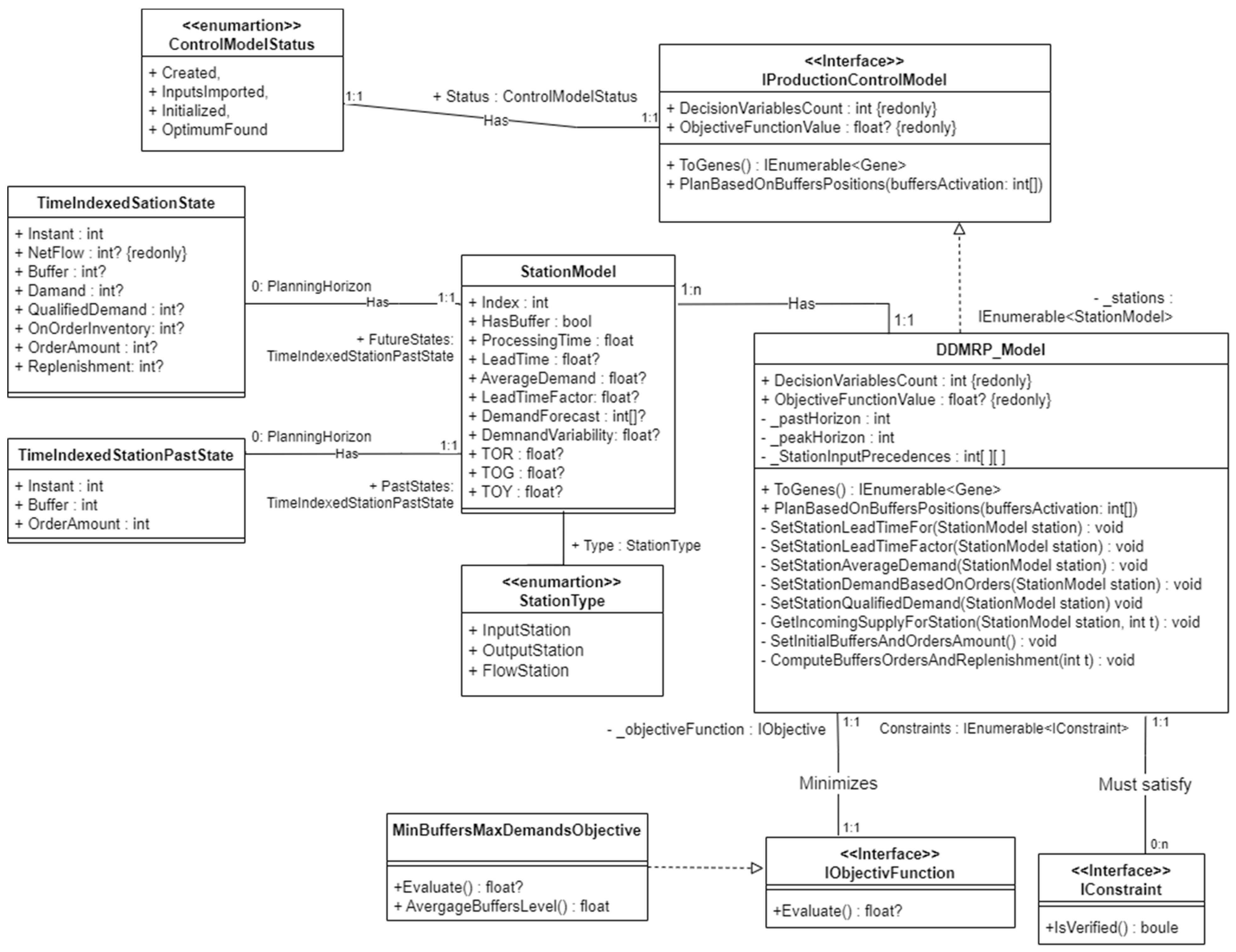
• The objective function, defining the optimization goal.
• The constraints, ensuring feasible solutions.
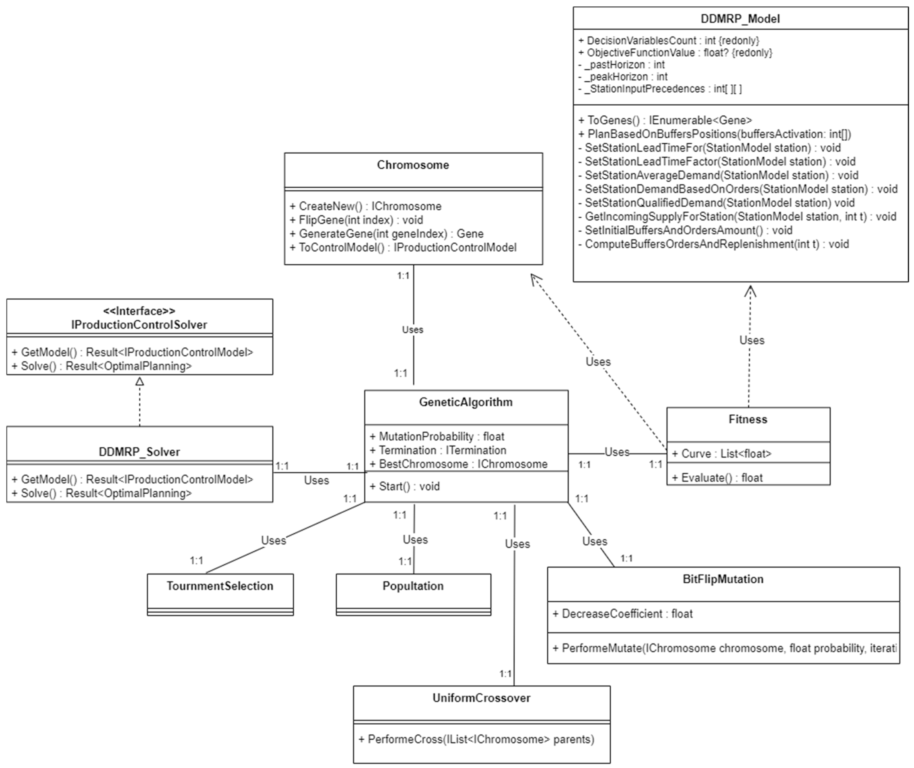
• A collection of Station Models (StationModel), representing individual production stations.
• Dependency constraints between these stations.

As each Station Model serves as an abstract representation of a station, it contains both general station data—such as its index—and DDRMP-related data, including average demand, demand variability, lead time, and Lead Time factor. It also contains TOR (Top of Red), TOG (Top of Green), and TOY (Top of Yellow), representing crucial DDMRP indicators.

Additionally, each Station Model maintains a history of past states and a set of future states, which are essential for optimization. Past states serve as initial input data, recording previous buffer sizes (if a buffer is present) and past order amounts. Future states, represented by the TimeIndexedStationState class, are time indexed and contains buffer size, demand, qualified demand, on order inventory, order amount, replenishment, and Net Flow indicator.

At initialization, a population of a solution is randomly generated, with buffers activated randomly as decision variables. Then DDMRP_Model class applies a set of methods to compute future station states based on the mathematical equations provided in Section 3. This is only executed when the fitness of a chromosome is evaluated.

As shown in Figure 5, the iterative optimization process is managed by the DDMRP_Solver class, which contains a Genetic Algorithm provided by GeneticSharp library [23]. This solver integrates:

• Chromosome and Fitness classes. Fitness class builds an instance of DDMRP_Model based on chromosome genes in order to evaluate the solution fitness when selection is performed.
• Tournament selection, provided by the library, for choosing individuals for reproduction.
• Population management, also based on built-in library classes.
• Built-in uniform crossover operator.
• Built-in Bit-Flip mutation operator.

For implementation, NET Core [35] was chosen due to its performance and cross-platform capabilities. As described in Section 3, the goal is to develop a Web Application Interface interoperable with a factory control system. The code developed is available at [36].

6. Case Study

In this section, a case study is presented to demonstrate the relevance and applicability of the proposed model. As illustrated in Figure 6, three different production line configurations are considered:

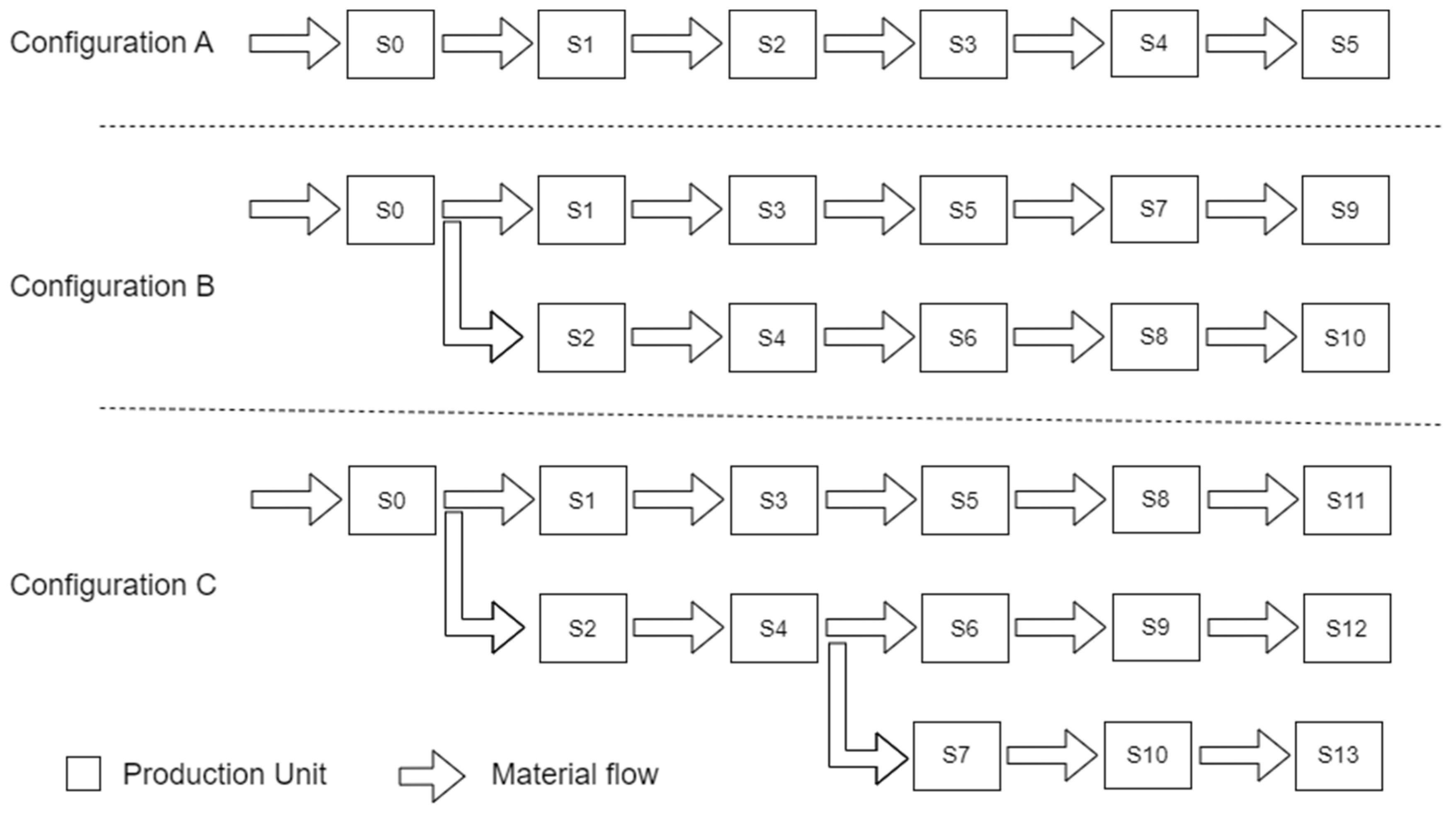
• Configuration A: Simple linear layout composed of six production units. The line is considered balanced, with a uniform processing time of 0.01 at each station. The demand is concentrated at output station S₅, with a total demand denoted by D_A. The number of possible configurations is $2^6=64$.
• Configuration B: Linear layout with a single ramification at station S₀, resulting in two branches. The line consists of eleven production units, with output stations located at S₉ and S₁₀. The demand is equally distributed between them and is denoted D_B = D_A/2. The processing time at S₀ is 0.01, while all other stations operate at 0.02 to maintain system balance. The number of possible configurations is $2^{11}=2048$.
• Configuration C: More complex layout featuring two ramifications, the first at S₀ and the second at S₄, resulting in three separate material flows. The layout remains balanced, with processing times set to 0.01 at S₀, 0.02 at stations S₁–S₄, and 0.03 at all subsequent stations. The demand at each output station is labeled D_C = D_A/3. The number of possible configurations is $2^{14}=\mathrm{16,348}$.

The planning horizon is set to 30 time units (TUs), with a past horizon of 3 and a Peak Horizon of 5. In the objective function (Equation (22)), the weights ω, λ, and δ are set respectfully to 10, 1, and 100. The Lead Time at Station 0 is set to 2 TUs.

Table 2. Demand forecast.

(a)
Date	0	1	2	3	4	5	6	7	8	9	10	11	12	13	14
Demand	80	30	50	120	150	70	100	45	60	120	130	80	50	70	106
(b)
Date	15	16	17	18	19	20	21	22	23	24	25	26	27	28	29
Demand	130	100	80	50	80	45	70	106	130	100	106	45	33	106	45

presents the demand forecast over the planning horizon. For configurations with multiple output stations (B and C), the demand is equally distributed among them:

To ensure comparable operating conditions across the three configurations, the demand variability was adjusted to satisfy: VC/3 = VB/2 = VA = 34%. Simulations were executed on a machine with 32 GB RAM and an Intel(R) Core(TM) Ultra 7 165H CPU@1.40 GHz. Initial population were set to 100 individuals. The average computation time observed before reaching fitness stagnation (threshold of 100 iterations) was approximately 1300 ms for configuration A, 2500 ms for configuration B, and 3100 ms for configuration C.

Figure 7 displays the evolution of objective functions for all three configurations. The curves show substantial improvements, reflecting optimal buffer stock levels and maximization of demand satisfaction across the planning horizon. Additionally, the resolution process generates the replenishment dates and order quantities for each buffered station using DDMRP principles. Configuration C detailed results are given in Appendix A.

Table 3. Overall production indicators.

Configuration	Optimal Buffer Positionings	Average Buffer Level	Average Unsatisfied Demand
A	1-1-0-0-0-1	442.3	13.5
B	1-1-0-0-0-0-0-0-1-0	254.4	11.7
C	1-1-0-1-0-0-0-0-1-0-0-0-0-0	194.3	11

summarizes the optimal buffer positioning and the corresponding average buffer levels and unsatisfied demand for each configuration:

Since station 0 is an outsourced operation with the longest Decoupled Lead Time, it naturally requires the placement of a buffer. Figure 8 illustrates stock level variations across the three production configurations. The results show that the algorithm dynamically adjusts inventory levels in response to demand fluctuations by effectively applying DDMRP principles. Notably, the variation in stock levels decreases progressively from one decoupling point to the next, indicating that the proposed planning method successfully absorbs upstream supply chain variability. Furthermore, the simulations suggest that branching within a configuration enhances overall system performance.

It is important to emphasize that all configurations in this study are balanced and the only source of variability modeled is demand fluctuation. To further evaluate the robustness of the proposed approach, future experiments should consider slightly unbalanced configurations. Additionally, incorporating plan-based disruptions that affect the balance would provide valuable insight into the algorithm’s capacity to support dynamic, real-time adjustments. These extensions represent promising directions for future research.

7. Conclusions

This study proposes a novel Mixed-Integer Linear Programming (MILP) formulation to operationalize the Demand-Driven Material Requirements Planning (DDMRP) methodology within a multi-stage production environment. The developed model captures dynamic interactions between external demand, buffer fluctuations, and replenishment decisions, while integrating core DDMRP principles such as Decoupled Lead Times and Net Flow indicator.

To solve this optimization problem characterized by non-linearities, recursive constraints, and mixed-integer decision variables a Genetic Algorithm (GA) is used. This metaheuristic incorporates a uniform crossover and bit-flip mutation operators, specifically adapted to the problem structure, as well as a dynamic mutation probability mechanism to maintain a balance between exploration and exploitation throughout the evolutionary process.

Although the proposed approach has not yet been implemented in a real industrial setting, it was designed with practical deployment in mind—particularly within reconfigurable manufacturing environments equipped with real-time data acquisition, feedback systems, and advanced automation capabilities. Such contexts, characterized by high variability and the need for adaptive planning, are especially well suited to the DDMRP methodology. Additionally, the simulation results demonstrate that the approach can generate effective solutions within a large solution space, achieving a theoretical balance between stock levels and robustness to demand variability. While its implementation in real-world industrial settings appears promising, it remains beyond the scope of the present study.

This research thus provides a solid theoretical foundation for future industrial applications of DDMRP in reconfigurable systems. To further enhance the model’s realism and applicability, future studies may extend it to account for additional sources of uncertainty beyond demand, such as:

• Human resources: This includes factors such as workforce skill levels, fatigue, shift schedules, and absenteeism, all of which influence production reliability and performance [37,38,39,40,41]. Moreover, the model introduced in this work can be integrated with simulation techniques to more effectively account for additional sources of variability beyond those related to external demand.
• Machine-related disruptions such as equipment breakdowns, maintenance cycles, or setup delays, which affect lead times and resource availability.

Capturing these operational uncertainties would require moving toward stochastic or scenario-based formulations. Additionally, the integration of rolling-horizon or real-time planning mechanisms could enhance the model’s responsiveness by dynamically adjusting decisions based on sensor data or updated system states.

Ultimately, these developments would support the creation of a robust and adaptive decision-support tool, fully aligned with Industry 4.0 requirements and dynamic production systems operating under the DDMRP framework.

References

1. Ptak, C.A.; Smith, C.; Orlicky, J.A. Orlicky’s Material Requirements Planning, 3rd ed.; Online-Ausg.; McGraw-Hill: New York, NY, USA, 2011; ISBN 978-0-07-175564-1. [Google Scholar]
2. Thürer, M.; Fernandes, N.O.; Stevenson, M. Production Planning and Control in Multi-Stage Assembly Systems: An Assessment of Kanban, MRP, OPT (DBR) and DDMRP by Simulation. Int. J. Prod. Res. 2022, 60, 1036–1050. [Google Scholar] [CrossRef]
3. Demand Driven Institute. Demand Driven Case Studies. Available online: https://www.demanddriveninstitute.com/case-studies (accessed on 6 April 2025).
4. Ptak, C.; Smith, C. Demand Driven Material Requirements Planning (DDMRP); Industrial Press, Inc.: New York, NY, USA, 2016; ISBN 978-0-8311-9384-3. [Google Scholar]
5. Azzamouri, A.; Baptiste, P.; Dessevre, G.; Pellerin, R. Demand Driven Material Requirements Planning (DDMRP): A Systematic Review and Classification. J. Ind. Eng. Manag. 2021, 14, 439. [Google Scholar] [CrossRef]
6. Marzougui, M.E.; Messaoudi, N.; Dachry, W.; Sarir, H.; Bensassi, B. Demand Driven MRP: Literature Review and Research Issues. 2020. Available online: https://hal.science/hal-03193163/ (accessed on 29 March 2025).
7. Pekarcıkova, M.; Trebuna, P.; Kliment, M.; Trojan, J. Demand Driven Material Requirements Planning. Some Methodical and Practical Comments. Manag. Prod. Eng. Rev. 2019, 10, 50–59. [Google Scholar] [CrossRef]
8. Favaretto, D.; Marin, A. An Empirical Comparison Study Between DDMRP and MRP in Material Management. SSRN J. 2018. [Google Scholar] [CrossRef]
9. Miclo, R.; Fontanili, F.; Lauras, M.; Lamothe, J.; Milian, B. An Empirical Comparison of MRPII and Demand-Driven MRP. IFAC-Pap. 2016, 49, 1725–1730. [Google Scholar] [CrossRef]
10. Shofa, M.J.; Widyarto, W.O. Effective Production Control in an Automotive Industry: MRP vs. Demand-Driven MRP; AIP Publishing: Surakarta, Indonesia, 2017; p. 020004. Available online: https://pubs.aip.org/aip/acp/article/815355 (accessed on 29 March 2025).
11. Damand, D.; Lahrichi, Y.; Barth, M. Parameterisation of Demand-Driven Material Requirements Planning: A Multi-Objective Genetic Algorithm. Int. J. Prod. Res. 2023, 61, 5134–5155. [Google Scholar] [CrossRef]
12. Achergui, A.; Allaoui, H.; Hsu, T. Optimisation of the Automated Buffer Positioning Model under DDMRP Logic. IFAC-Pap. 2021, 54, 582–588. [Google Scholar] [CrossRef]
13. Velasco Acosta, A.P.; Mascle, C.; Baptiste, P. Applicability of Demand-Driven MRP in a Complex Manufacturing Environment. Int. J. Prod. Res. 2020, 58, 4233–4245. [Google Scholar] [CrossRef]
14. Lee, C.-J.; Rim, S.-C. A Mathematical Safety Stock Model for DDMRP Inventory Replenishment. Math. Probl. Eng. 2019, 2019, 6496309. [Google Scholar] [CrossRef]
15. Trigueiro De Sousa Junior, W.; Barra Montevechi, J.A.; De Carvalho Miranda, R.; Teberga Campos, A. Discrete Simulation-Based Optimization Methods for Industrial Engineering Problems: A Systematic Literature Review. Comput. Ind. Eng. 2019, 128, 526–540. [Google Scholar] [CrossRef]
16. El Marzougui, M.; Messaoudi, N.; Dachry, W.; Bensassi, B. Industry 4.0 Technologies on Demand Driven Material Requirement Planning: Theoretical Background and Impacts. In Proceedings of the International Conference on Advanced Intelligent Systems for Sustainable Development; Kacprzyk, J., Ezziyyani, M., Balasy, V.E., Eds.; Springer Nature: Cham, Switzerland, 2023; pp. 59–69. [Google Scholar]
17. Marzougui, M.E.; Messaoudi, N.; Dachry, W.; Bensassi, B. Integration Model for Demand-Driven Material Requirement Planning and Industry 4.0. SAE Int. J. Mater. Manuf. 2022, 16, 3–14. [Google Scholar] [CrossRef]
18. ASCM. Association for Supply Chain Management—ASCM. Available online: https://www.ascm.org/ (accessed on 27 December 2024).
19. Llamuca, E.S.; Garcia, C.A.; Naranjo, J.E.; Garcia, M.V. Cyber-Physical Production Systems for Industrial Shop-Floor Integration Based on AMQP; IEEE: Piscataway, NJ, USA, 2019. [Google Scholar]
20. Haji Mohammad, F.; Benali, M.; Baptiste, P. An Optimization Model for Demand-Driven Distribution Resource Planning DDDRP. J. Ind. Eng. Manag. 2022, 15, 338. [Google Scholar] [CrossRef]
21. Reid, D.J. Genetic Algorithms in Constrained Optimization. Math. Comput. Model. 1996, 23, 87–111. [Google Scholar] [CrossRef]
22. Zou, Z.; Li, C. Integrated and Events-Oriented Job Shop Scheduling. Int. J. Adv. Manuf. Technol. 2006, 29, 551–556. [Google Scholar] [CrossRef]
23. Giacomelli/GeneticSharp. GeneticSharp Is a Fast, Extensible, Multi-Platform and Multithreading C# Genetic Algorithm Library that Simplifies the Development of Applications Using Genetic Algorithms (GAs). Available online: https://github.com/giacomelli/GeneticSharp (accessed on 5 April 2025).
24. Goldberg, D.E.; Holland, J.H. Genetic Algorithms and Machine Learning. Mach. Learn. 1988, 3, 95–99. [Google Scholar] [CrossRef]
25. Holland, J.H. Adaptation in Natural and Artificial Systems; The MIT Press: Cambridge, MA, USA, 1992; ISBN 978-0-262-58111-0. [Google Scholar]
26. Deb, K. Multi-Objective Optimization Using Evolutionary Algorithms|Wiley; Wiley: Hoboken, NJ, USA, 2001; ISBN 978-0-471-87339-6. [Google Scholar]
27. Mitchell, M. An Introduction to Genetic Algorithms; MIT Press: Cambridge, MA, USA, 1998; ISBN 978-0-262-63185-3. [Google Scholar]
28. Kacem, I.; Hammadi, S.; Borne, P. Approach by Localization and Multiobjective Evolutionary Optimization for Flexible Job-Shop Scheduling Problems. IEEE 2002, 32, 1–13. [Google Scholar] [CrossRef]
29. Yeniay, Ö. Penalty Function Methods for Constrained Optimization with Genetic Algorithms. Math. Comput. Appl. 2005, 10, 45–56. [Google Scholar] [CrossRef]
30. Deb, K. An Efficient Constraint Handling Method for Genetic Algorithms. Comput. Methods Appl. Mech. Eng. 2000, 186, 311–338. [Google Scholar] [CrossRef]
31. Gen, M.; Cheng, R. Genetic Algorithms and Engineering Optimization; John Wiley & Sons: Hoboken, NJ, USA, 1999; ISBN 978-0-471-31531-5. [Google Scholar]
32. Lu, Y.; Benlic, U.; Wu, Q. A Hybrid Evolutionary Algorithm for the Capacitated Minimum Spanning Tree Problem. Comput. Oper. Res. 2022, 144, 105799. [Google Scholar] [CrossRef]
33. Millett, S.; Tune, N. Patterns, Principles, and Practices of Domain-Driven Design; Wiley: Hoboken, NJ, USA, 2015; ISBN 978-1-118-71470-6. [Google Scholar]
34. UML Class and Object Diagrams Overview—Common Types of UML Structure Diagrams. Available online: https://www.uml-diagrams.org/class-diagrams-overview.html (accessed on 26 June 2025).
35. Gewarren Introduction to .NET-.NET. Available online: https://learn.microsoft.com/en-us/dotnet/core/introduction (accessed on 4 April 2025).
36. El Mouayni, I. ismail-elmouayni/SmartPPC: SmartPPC a DDMRP based Production Planning and Control Module. Available online: https://github.com/ismail-elmouayni/SmartPPC (accessed on 5 April 2025).
37. Dantan, J.-Y.; El Mouayni, I.; Sadeghi, L.; Siadat, A.; Etienne, A. Human Factors Integration in Manufacturing Systems Design Using Function–Behavior–Structure Framework and Behaviour Simulations. CIRP Ann. 2019, 68, 125–128. [Google Scholar] [CrossRef]
38. El Mouayni, I.; Etienne, A.; Siadat, A.; Dantan, J.-Y.; Lux, A. A Simulation Based Approach for Enhancing Health Aspects in Production Systems by Integrating Work Margins. IFAC-Pap. 2016, 49, 1697–1702. [Google Scholar] [CrossRef]
39. El Mouayni, I.; Etienne, A.; Siadat, A.; Dantan, J.-Y.; Lux, A. AEN-PRO: Agent-Based Simulation Tool for Performance and Working Conditions Assessment in Production Systems Using Workers’ Margins of Manoeuver. IFAC-Pap. 2017, 50, 14236–14241. [Google Scholar] [CrossRef]
40. Mouayni, I.E.; Demesure, G.; Haouzi, H.B.-E.; Charpentier, P.; Siadat, A. Jobs Scheduling within Industry 4.0 with Consideration of Worker’s Fatigue and Reliability Using Greedy Randomized Adaptive Search Procedure. IFAC-Pap. 2019, 52, 85–90. [Google Scholar] [CrossRef]
41. El Mouayni, I.; Etienne, A.; Lux, A.; Siadat, A.; Dantan, J.-Y. A Simulation-Based Approach for Time Allowances Assessment during Production System Design with Consideration of Worker’s Fatigue, Learning and Reliability. Comput. Ind. Eng. 2020, 139, 105650. [Google Scholar] [CrossRef]
Figure 1. Illustration of decoupling points effect on production variability [4].
Jmmp 09 00219 g001
Figure 2. Production Planning and Control (PPC) integration architecture.
Jmmp 09 00219 g002
Figure 3. Illustration of a production configuration.
Jmmp 09 00219 g003
Figure 4. UML class diagram of domain layer [34]: Production Planning Control Model.
Jmmp 09 00219 g004
Figure 5. Class diagram of domain layer [34]- Production Planning Control Solver.
Jmmp 09 00219 g005
Figure 6. Production configurations under study.
Jmmp 09 00219 g006
Figure 7. Objective function improvement for configurations (AC).
Jmmp 09 00219 g007
Figure 8. (A): Stock variation in stations S0, S1 and S5 of configuration A for. (B): Stock variation in stations S0, S1 and S9 of configuration B. (C): Stock variation in stations S0, S1, S3 and S8 of configuration C.
Jmmp 09 00219 g008