Optimization of Machining Parameters for the Fixed Pocket Cycle

Abstract

In a competitive industrial setting, optimizing machining processes is important for enhancing surface quality and productivity. This study focuses on optimizing pocket milling parameters for 5083 H111 aluminum alloy using three toolpath strategies: Zig-Zag, Parallel Spiral, and One-Way. To achieve these goals, the Taguchi method, Grey Relational Analysis (GRA), ANOVA, and visual amplification were employed to evaluate the influence of cutting speed (V_c), feed per tooth (f_z), and axial depth of cut (a_p) on surface roughness and production rate. For the Zig-Zag and Parallel Spiral tool paths, cutting speed was the most important factor affecting surface roughness. For the One-Way strategy, axial penetration was the most important factor. The Parallel Spiral toolpath, under the V_c of 150 m/min, the f_z of 0.025 mm/tooth, and the a_p of 1.0 mm (A3-B3-C1) configuration, achieved the best balance between surface finish and production rate. Visual analysis also showed significative differences in how rough the wall was along perpendicular and parallel tool paths, which made it clear that finishing passes are needed in some cases. This research shows that using both statistical methods and visual amplification together makes process optimization more organized and effective, which leads to better machining performance.

1. Introduction

In a competitive global market, manufacturing industries must continuously optimize their processes to meet high-quality standards and economic demands [1]. Machining processes, particularly milling, play an important role in producing complex geometries with high precision across various materials [2]. Among these, pocket milling is widely used in die and mold manufacturing, where surface roughness directly impacts functional properties, such as wear resistance and coating adhesion [3,4].

To keep-in par with the market, the optimization of machining parameters is essential, such as cutting speed, feed rate, and depth of cut, along with tool path strategies, which play a crucial role in determining surface roughness. Previous studies have shown that optimizing machining parameters can greatly enhance surface finish [5], demonstrating that optimized machining conditions could improve surface roughness by 250% [6], while finding that depth of cut had a lesser influence compared to cutting speed and feed rate. Balaji et al. and Davim [7,8] identified spindle speed, feed rate, and cutting velocity as dominant factors in surface quality, whereas Nalbant et al. [9] emphasized the role of insert radius and feed over depth of cut.

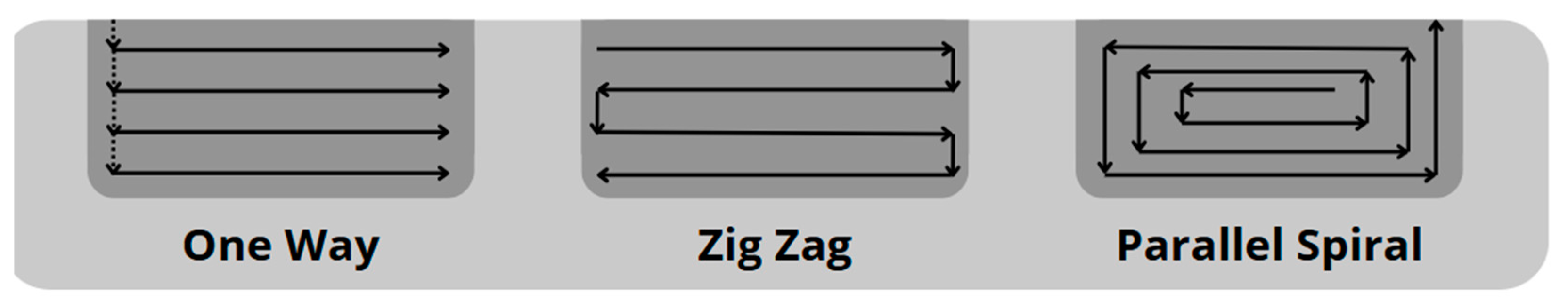
Tool path strategies have gained attention as a key factor influencing machining performance and surface integrity. Studies have shown how workpiece inclination and cutting speed affect cutting forces, tool deflection, and roughness [10,11,12], while Lazoglu et al. [13] optimized tool paths for freeform machining, showing that One-Way and Zig-Zag strategies provided superior results over Spiral paths. Further studies highlighted that the inclination angle had the most significant effect on surface roughness in multi-axis milling, followed by feed rate and cutting speed [14]. Abdulrazaq et al. [15] conducted a study to identify the optimal combination of machining parameters for maximizing production efficiency and minimizing surface roughness, employing the Taguchi method in conjunction with ANOVA statistical analysis. Upadrashta et al. [16] conducted a similar analysis on a heat-treated magnesium alloy, exploring how variations in cutting depth, feed rate, and cutting speed influenced the machining process. Another study presented by Ribeiro et al. [17] demonstrates that the Taguchi method can be effectively applied to different machining process types, focusing on the influence of the feed rate variation in the burnishing process. These findings indicate the importance of selecting appropriate tool paths and machining conditions to achieve optimal surfaces in machining.

Taguchi’s method [18] provides a structured approach to experimental design using orthogonal arrays, enabling the identification of optimal cutting parameters for individual performance criteria, such as surface roughness [19]. However, Grey Relational Analysis (GRA) becomes a valuable tool when evaluating multiple quality characteristics, as it ranks parameter combinations according to their relative significance [20]. Integrating these methods with Analysis of Variance (ANOVA) enables a comprehensive evaluation of parameter effects and facilitates effective process optimization.

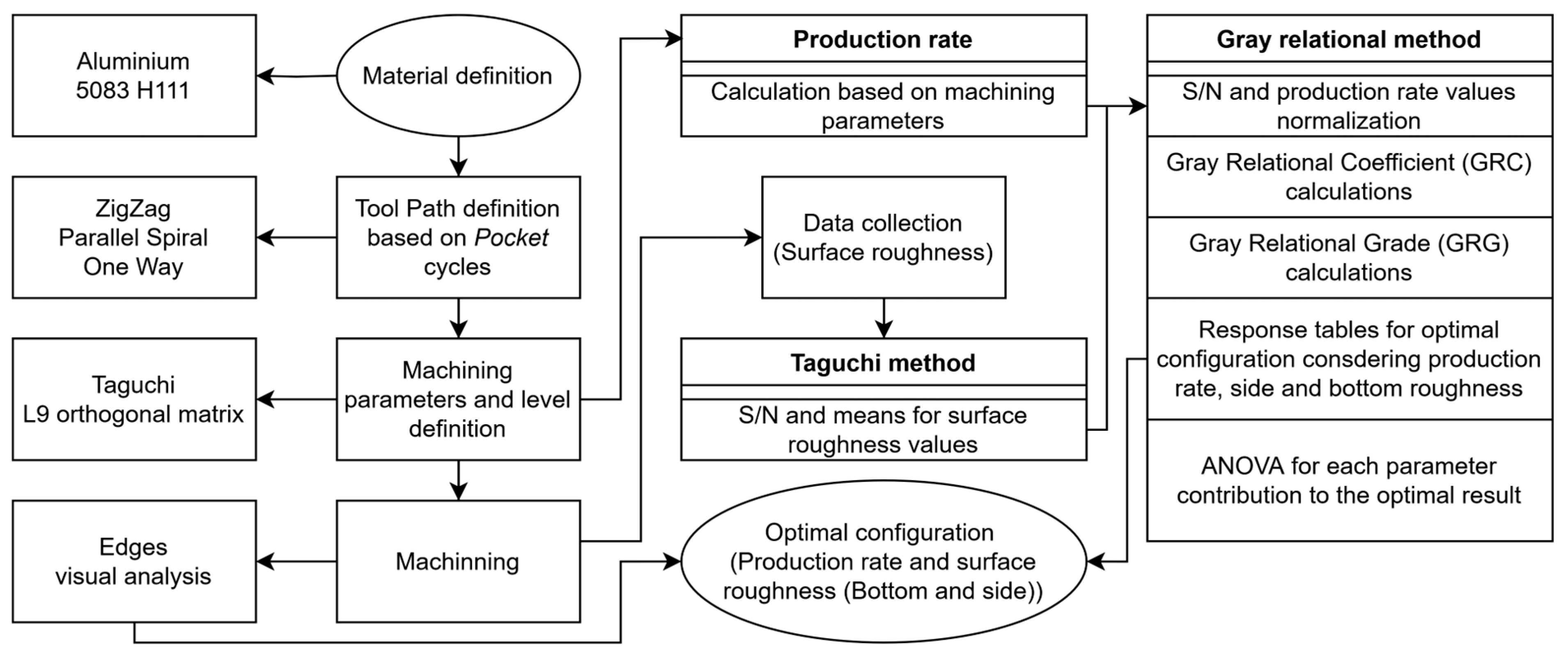
This study aims to optimize pocket milling parameters to minimize surface roughness and maximize the production rate of the 5083 H111 aluminum alloy, with particular emphasis on the machined pocket walls. Three toolpath strategies are evaluated using the Taguchi method and Grey Relational Analysis (GRA), while ANOVA is employed to assess the statistical significance of each parameter. The key contribution of this work is the in-depth analysis of the machined lateral walls, highlighting how different toolpath strategies affect the final surface finish.

2. Materials and Methods

Figure 1 presents a flowchart outlining the workflow of this study. The process began with the selection of the material, followed by the definition of tool paths based on pocket milling cycles. Subsequently, a Taguchi method was employed to establish machining parameter variations, enabling the calculation of the production rate and the related orthogonal array. After the planning phase and the parameters definition, the milling process was conducted, followed by roughness measurements and visual analysis. Finally, with all data collected, a comprehensive evaluation was performed to determine the optimal set of parameters for maximizing both production and surface quality.

2.1. Material Selection

The material selected for this study was the 5083 H111 aluminum alloy, using 35 mm × 35 mm × 150 mm billets. This alloy contains at least 4% magnesium, which enhances its weldability and provides superior corrosion resistance. In its designation, the letter “H” indicates that the material has undergone strain hardening, with the first digit denoting the method, where “1” signifies cold working, and the second digit indicating a low degree of hardness. Due to its excellent mechanical properties and resistance to harsh environments, this alloy is widely used in the naval industry. The material mechanical properties and chemical composition are presented in

Table 1. Mechanical properties of 5083 H111 aluminum alloy [21].

Propriety	Value
Density [g/cm3]	2.8
Young’s Modulus [MPa]	70,000
Yield Strength [MPa]	125
Ultimate Tensile Strength [MPa]	270–345
Elongation [%]	15
Hardness [2.5/62.5]	70

and

Table 2. Chemical composition of 5083 H111 aluminum alloy [21].

Element	Minimum [%]	Maximum [%]
Si	-	0.4
Fe	-	0.4
Cu	-	0.1
Mn	0.4	0.1
Mg	4	4.9
Cr	0.05	0.25
Zn	-	0.25
Ti	-	0.15
Other	0.05	0.15
Al	Remaining	Remaining

, respectively.

2.2. Decision Parameters

The Computer Numerical Control (CNC) milling process offers various machining strategies, and selecting the most suitable approach for a given application directly influences dimensional accuracy, surface roughness, and tool wear. One of the most widely used fixed cycles is pocket milling, known for its versatility and broad application across industries such as automotive and aerospace. To machine the samples, three distinct tool paths were implemented: Zig-Zag (Z), Parallel Spiral (S), and One-Way (O), as illustrated in Figure 2. These tool paths were chosen due to their widespread use in industrial applications.

2.3. Equipment

The CNC milling machine employed in this study was the Deckel Maho DMC (DMG Mori, Bielefeld, Germany) 63 V (Figure 3) and Seco^® JSE514060D2C.0Z4 SIRA for the cutting tool. Surface roughness measurements were conducted using a Mitutoyo^® SJ-301, which was used to measure and determine the roughness values from both the bottom and lateral surfaces under 0.8 mm of cut-off, at a velocity of 0.5 mm/s. For optical analysis, a Veho VMS-005-LCD was utilized to evaluate the lateral roughness with a 20-times magnification, as its higher roughness exceeded the resolution capability of the surface roughness device.

2.4. Taguchi

Taguchi emphasized that incorporating quality concepts at the design stage is more effective than relying on post-manufacturing inspection [18]. The Taguchi method optimizes processes to minimize quality loss using objective functions such as “nominal-the-best”, “larger-the-better”, or “smaller-the-better”, depending on the experimental goal. In machining, this method systematically evaluates cutting parameters to enhance surface quality and process efficiency. Taguchi categorizes design into three stages: system design, parameter design, and tolerance design. System design defines the overall process framework, parameter design identifies optimal machining settings, and tolerance design establishes acceptable deviations. Among these, parameter design is critical in achieving robust machining conditions by reducing variability, referred to as noise, in the process [22].

2.4.1. Process Parameter Selection

Surface roughness and production rate are critical factors in machining processes. One of the main objectives in industrial machining is to achieve the lowest possible surface roughness while maintaining a high material removal/rate. To optimize these characteristics, the most commonly adjusted machining parameters include cutting speed (V_c), feed per tooth (f_z), and axial depth of cut (a_p). For this study, the selection of process parameters was based on the manufacturer’s recommendations (maximum, minimum, and intermediate) for the specific cutting tool (Seco^® JSE514060D2C.0Z4 SIRA) used in this work. Based on these limitations, the selected parameters and their levels are summarized in

Table 3. Process parameters with their range and values at three levels.

Parameters	Range	Level 1	Level 2	Level 3
Cutting speed [m/min] (A)	50–150	50	100	150
Feed per tooth [mm/tooth] (B)	0.025–0.035	0.035	0.030	0.025
Depth of cut [mm] (C)	1–2	1.0	1.5	2.0

.

Given that three machining parameters were chosen, each with three levels, the recommended orthogonal array for this experiment, following the Taguchi method, is the L9 orthogonal array.

2.4.2. Material Removal Rate

In machining operations, process parameter calculations are not always required solely for manufacturing purposes but also for evaluating productivity. In milling, productivity can be assessed by measuring the volume of material removed over a given time. This efficiency metric is commonly defined by the Material Removal Rate (MRR), which is calculated using the following equation:

$$MRR=a_e\ast a_p\ast V_f$$

(1)

where MRR is the Material Removal Rate (mm³/min), a_e is the width of cut (mm), a_p is the depth of cut (mm) and V_f is the feed rate (mm/min). This equation provides a straightforward method for quantifying machining efficiency, allowing for a direct comparison of different cutting conditions and toolpath strategies.

2.4.3. Optimization Techniques

The signal-to-noise (S/N) ratio was calculated to quantitatively assess the impact of each process variable on the response. For cases where the objective is to minimize the response variable, like in the surface roughness, the smaller-the-better S/N ratio formulation was applied, while for maximization, the larger-the-better approach can be used, for example, maximizing the Material Removal Rate (MRR) [23,24]. The S/N ratio for smaller-the-better is determined as follows:

$${\displaystyle \frac{S}{N_S}}=-10·\mathrm{l}\mathrm{o}\mathrm{g}\left({\displaystyle \frac{1}{n}}\ast {\displaystyle {\sum }_{i=1}^n}{Y}_i^2\right)$$

(2)

To maximize the output, larger-the-better is as follows:

$${\displaystyle \frac{S}{N_L}}=-10·\mathrm{l}\mathrm{o}\mathrm{g}\left({\displaystyle \frac{1}{n}}\ast {\displaystyle {\sum }_{i=1}^n}{\displaystyle \frac{1}{Y_i^2}}\right)$$

(3)

where n represents the number of observations and Y_i represents the data from each observation. These formulations enable a systematic evaluation of the effects of process parameters, thereby facilitating improved process optimization.

2.5. Grey Relational Analysis

2.5.1. Data Preprocessing

In Grey Relational Analysis (GRA), data preprocessing is essential for converting raw data into a comparable sequence. The choice of preprocessing method depends on the nature of the original data and the desired optimization objective [25,26]. When the objective is to maximize the response variable (larger-the-better), the original sequence is normalized using the following transformation:

$$x_{ij}={\displaystyle \frac{n_{ij}-\min n_{ij} }{\max n_{\mathit{ij}}-\min n_{ij}}}$$

(4)

If the purpose is to minimize (smaller-the-better), then the equation is as follows:

$$x_{ij}={\displaystyle \frac{{\max n_{ij}-n}_{ij} }{\max n_{\mathit{ij}}-\min n_{ij}}}$$

(5)

where $n_{ij}$ is the signal-to-noise ratio obtained from the Taguchi method, $\max n_{ij}$ is the maximum value of the signal-to-noise ratio, and $\min n_{ij}$ is the minimal value for the signal-to-noise ratio; the normalization must be performed for all quality characteristics that will be considered.

2.5.2. Grey Relational Coefficients and Grades

After data preprocessing, the Grey Relational Coefficient (GRC) is computed using the normalized sequences. The GRC quantifies the relationship between the reference sequence and each comparability sequence and is defined as follows [27]:

$${\mathrm{\xi }}_{ij}={\displaystyle \frac{\mathrm{m}\mathrm{i}\mathrm{n}∆+\mathrm{\zeta } \mathrm{m}\mathrm{a}\mathrm{x}∆ }{{∆}_{ij}+\mathrm{\zeta } \mathrm{m}\mathrm{a}\mathrm{x} ∆}}$$

(6)

where ξ_ij represents the GRC, ${∆}_{ij}$ = |$x_0$(k) − $x_i$(k)| is the absolute difference between the reference and comparability sequences, and ζ is the distinguishing coefficient. For this study, the number of evaluated quality components is 3 (side roughness, bottom roughness, and MMR).

The Grey Relational Grade (GRG) is then obtained as a weighted sum of the GRC:

$${\mathrm{\gamma }}_i={\displaystyle \frac{1}{n}}\ast {\displaystyle {\sum }_{k=1}^n}{\mathrm{\xi }}_{ij}$$

(7)

where γ_i represents the overall correlation between the reference sequence and the comparability sequence. The GRG also reflects the degree of influence exerted by a comparability sequence on the reference sequence; higher values indicate a stronger relationship. As a result, if a particular comparability sequence has a greater impact on the reference sequence than others, its GRG will be higher.

2.5.3. Confirmation Test

In cases where the optimal parameter combination identified by the Grey Relational Analysis (GRA) does not correspond to any of the experimental runs in the Taguchi orthogonal array, a confirmation test is required. This test evaluates the extent to which the Taguchi method contributes to improving the process.

Using the optimal parameter levels determined by GRA, the estimated GRG is calculated as follows:

$$\widehat{n}=n_m{\displaystyle {\sum }_{i=1}^q}(\overline{n_i}-n_m)$$

(8)

where $\widehat{n}$ is the estimated GRG for the optimal parameter combination, n_m is the overall mean GRG across all experiments for the select sample, $\overline{n_i}$ is the GRG for the optimal level of each parameter, and q is the number of significant parameters influencing the process.

This calculation helps assess the validity of the predicted optimal settings and ensures that the selected combination effectively enhances machining performance. If necessary, additional experimental validation is conducted to confirm the predicted improvements by redoing the steps for the signal-to-noise ratio from Taguchi and the steps from Grey Relational Analysis for the validation sample.

2.6. ANOVA Analysis

ANOVA analysis was used to assess the impact of machining parameters on surface roughness and production rate. We determined the statistical significance for each factor and ranked their influence on the machining response. This analysis validated the results obtained through the Taguchi method, confirming the optimal parameter combination. Taguchi, ANOVA, and the response table analyses were conducted using Minitab^TM 17 statistical software.

3. Results

Using the parameters outlined in Table 1, the L9 orthogonal array proposed by the Taguchi method [15] can be constructed, incorporating the parameter variations required for the experimental accomplishment.

Table 4. L9 Orthogonal configuration with its respective MMR.

Sample	L9—Orthogonal	Vc	Fz	ap	MRR
	Configuration	[m/min]	[mm/t]	[mm]	[mm3/min]
1	A1-B1-C1	50	0.035	1.00	740
2	A1-B2-C2	50	0.030	1.50	960
3	A1-B3-C3	50	0.025	2.00	1060
4	A2-B1-C2	100	0.035	1.50	2230
5	A2-B2-C3	100	0.030	2.00	2550
6	A2-B3-C1	100	0.025	1.00	1060
7	A3-B1-C3	150	0.035	2.00	4460
8	A3-B2-C1	150	0.030	1.00	1910
9	A3-B3-C2	150	0.025	1.50	2390

presents the L9 orthogonal configuration, detailing the parameter settings for each sample. Since the experimental design is structured around individual toolpaths, each selected toolpath corresponds to a set of nine experimental samples, with a total of 27 experimental samples, ensuring a systematic evaluation of machining conditions.

Table 4 also presents the Material Removal Rate (MRR) corresponding to each L9 orthogonal configuration. The MRR values were computed using Equation (1).

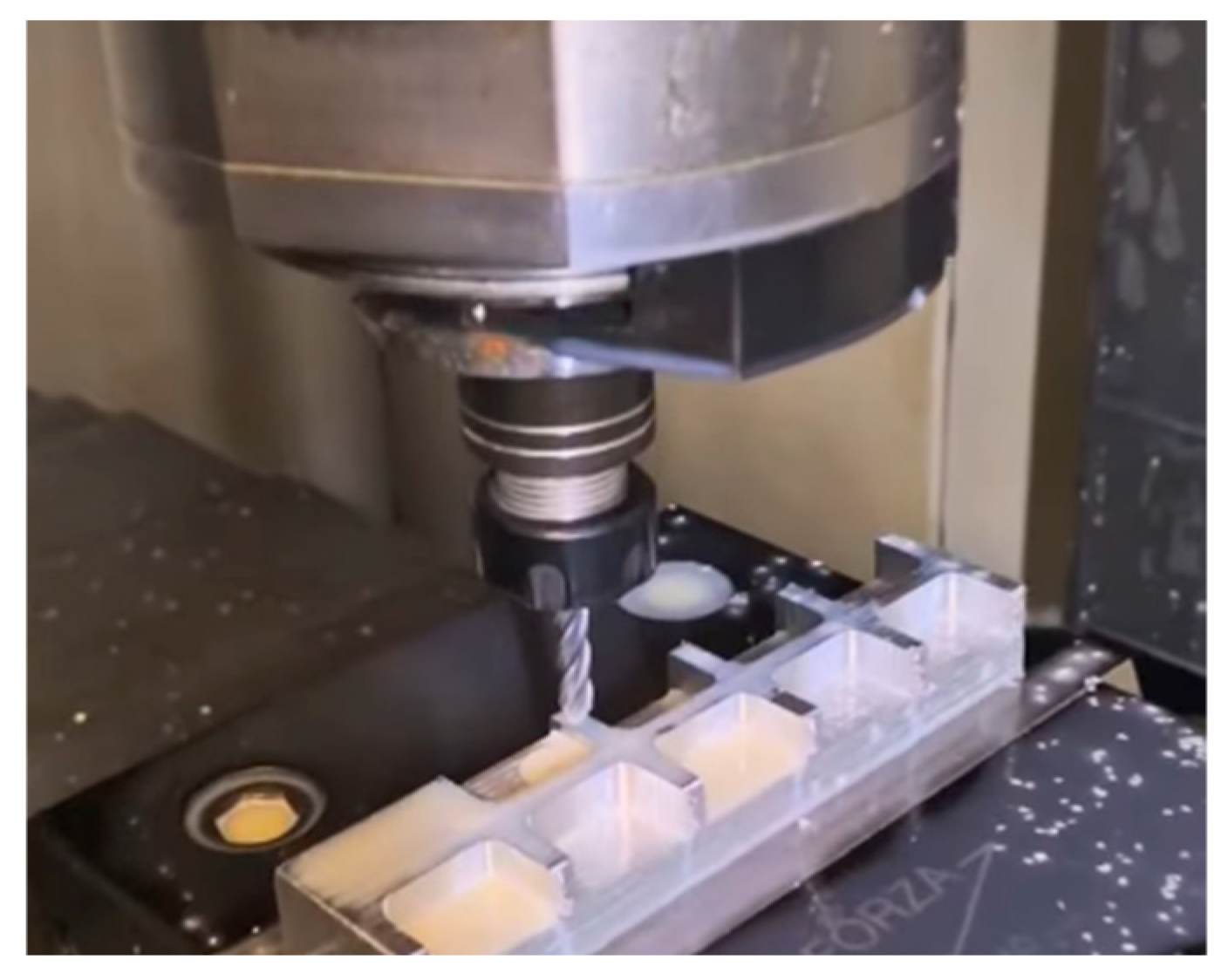
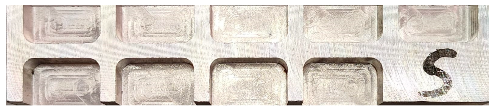
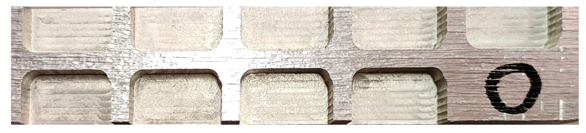
Following the parameters outlined in Table 3, the CNC milling process can be carried out, and the resulting machined samples can be observed in Figure 4, Figure 5 and Figure 6.

3.1. Surface Roughness

Surface roughness measurements were obtained using the Mitutoyo SJ-301 roughness tester (Mytutoyo, Kanagawa, Japan), with fourteen independent observations recorded for each pocket, systematically divided between side and bottom, as schematically illustrated in Figure 7. This extensive dataset enabled the application of the Taguchi method, where the signal-to-noise (S/N) ratio for each pocket was computed using Equation (2), following the “smaller-the-better” criterion, which is generally preferred for surface roughness optimization.

Table 5. S/N ratio (SN) for bottom (B) and side (S) values for each sample and toolpath (Z, S and O).

Sample	SN-Z_B	SN-Z_S	SN-S_B	SN-S_S	SN-O_B	SN-O_S
1	−7.55	2.09	−6.47	−0.76	−6.28	−1.81
2	−7.62	1.34	−7.58	0.49	−6.28	−1.71
3	−6.32	1.30	−6.57	−1.21	−5.53	−1.52
4	−7.39	0.76	−7.47	0.34	−7.42	0.21
5	−6.72	0.85	−6.32	−0.95	−6.92	−1.38
6	−6.97	0.97	−4.25	1.06	−7.89	−1.15
7	−6.74	2.98	−7.03	−1.58	−8.56	−1.66
8	−6.97	2.89	−5.45	1.29	−8.39	−0.74
9	−3.89	−1.24	−5.56	1.14	−7.44	−1.30

presents the signal-to-noise (S/N) ratio values corresponding to each measured parameter. Each column is labelled according to the type of data it represents, where the S/N ratio is (SN), the toolpath strategy used (Z, S, or O), and the measurement location (bottom (B) or side (S)). This column nomenclature method will be consistently applied throughout the manuscript to ensure clarity and coherence in data presentation.

3.2. Grey Relational Analysis

By using the S/N ratios for bottom and side roughness, along with the production rate, the Grey Relational Analysis (GRA) can be applied to determine the optimal parameter configuration for maximizing both surface quality and productivity. To ensure the proper implementation of the Grey method, a data normalization process must be conducted using the S/N values for surface roughness (bottom and side presented in Table 5) and the material removal rate (MRR presented in Table 4). Since the S/N ratio values are negative, the larger-the-better normalization, Equation (4), was selected to ensure consistency, where values closer to zero are considered optimal related to the S/N ratios. The normalized data are presented in

Table 6. Normalized data, Grey Relational Coefficient, and grade.

Sample		N-B	N-S	N-MRR	GRC-B	GRC-S	GRC-MRR	GRG	Order
Z	1	0.017	0.789	0.000	0.253	0.612	0.250	0.372	4
	2	0.000	0.611	0.059	0.250	0.462	0.262	0.324	8
	3	0.347	0.603	0.086	0.338	0.456	0.267	0.354	6
	4	0.060	0.473	0.401	0.262	0.388	0.357	0.336	7
	5	0.240	0.497	0.487	0.305	0.398	0.394	0.366	5
	6	0.173	0.523	0.086	0.287	0.411	0.267	0.322	9
	7	0.235	1.000	1.000	0.303	1.000	1.000	0.768	1
	8	0.175	0.978	0.315	0.288	0.937	0.327	0.517	3
	9	1.000	0.000	0.444	1.000	0.250	0.375	0.542	2
S	1	0.331	0.285	0.000	0.333	0.318	0.250	0.300	8
	2	0.000	0.723	0.059	0.250	0.547	0.262	0.353	6
	3	0.303	0.130	0.086	0.323	0.277	0.267	0.289	9
	4	0.031	0.669	0.401	0.256	0.501	0.357	0.372	5
	5	0.377	0.219	0.487	0.349	0.299	0.394	0.347	7
	6	1.000	0.922	0.086	1.000	0.810	0.267	0.692	1
	7	0.162	0.000	1.000	0.285	0.250	1.000	0.512	4
	8	0.640	1.000	0.315	0.481	1.000	0.327	0.603	2
	9	0.605	0.948	0.444	0.458	0.864	0.375	0.566	3
O	1	0.752	0.000	0.000	0.573	0.250	0.250	0.358	6
	2	0.752	0.052	0.059	0.574	0.260	0.262	0.365	5
	3	1.000	0.143	0.086	1.000	0.280	0.267	0.516	2
	4	0.376	1.000	0.401	0.348	1.000	0.357	0.569	1
	5	0.541	0.216	0.487	0.421	0.298	0.394	0.371	4
	6	0.220	0.329	0.086	0.299	0.332	0.267	0.300	9
	7	0.000	0.076	1.000	0.250	0.265	1.000	0.505	3
	8	0.055	0.530	0.315	0.261	0.415	0.327	0.334	8
	9	0.371	0.254	0.444	0.346	0.309	0.375	0.343	7

, columns N-B, N-S, and N-MRR.

Following the Grey method, the Grey Relational Coefficient (GRC) was computed based on the normalized data using Equation (6), considering a distinguishing coefficient ζ = 1/3, which assigns equal importance to all optimization parameters. The GRC values are presented in Table 6, columns GRC-B, GRC-S, and GRC-MRR.

Finally, the Grey Relational Grade (GRG) was determined using Equation (7), quantifying the significance of each sample within its respective toolpath configuration. The results for GRG and the ranking order of significance for each toolpath strategy are systematically presented in Table 6.

Based on the GRG values presented in Table 4, the optimal parameters for each toolpath strategy can be ranked. This ranking is achieved by constructing a response table, where the highest GRG value is identified for each parameter within its respective toolpath. Table 6 presents the response data for each parameter, segmented by toolpath, providing a structured approach to determining the optimal machining conditions.

From Table 5, the optimal parameter configurations for each toolpath strategy can be identified for optimizing surface roughness (bottom and side) and material removal rate (MRR). For the Z toolpath, the optimal configuration is Vc = 150 m/min, fz = 0.035 mm/tooth, and ap = 2.0 mm (A3-B1-C3), which corresponds to Sample 7 in Table 4. Since this parameter combination was already tested within the L9 orthogonal array, no further confirmation is required for the Z toolpath.

For the S toolpath, the optimal configuration is Vc = 150 m/min, fz = 0.025 mm/tooth, and ap = 1.0 mm (A3-B3-C1), which was not included in the L9 orthogonal array. Consequently, a confirmation test is essential to verify its efficacy, as outlined in the Confirmation section. Lastly, for the O toolpath, the optimal configuration is A3-B1-C3, which is also present in Table 4 as part of the L9 orthogonal configuration, eliminating the need for additional confirmation testing.

Table 7. Response tables for the Grey Relational Grade.

		Level 1	Level 2	Level 3	Rank	Average
Z	Vc (A)	0.3500	0.3411	0.6089	1	0.433
	fz (B)	0.4917	0.4025	0.4058	3
	ap (C)	0.4037	0.4005	0.4958	2
S	Vc (A)	0.3141	0.4703	0.5599	1	0.448
	fz (B)	0.3945	0.4342	0.5157	3
	ap (C)	0.5317	0.4300	0.3827	2
O	Vc (A)	0.4129	0.3942	0.4130	3	0.407
	fz (B)	0.4771	0.3568	0.3862	2
	ap (C)	0.3305	0.4256	0.4639	1

presents the results for the analysis of variance for the GRG; considering the contribution portion of each parameter, for the Z and S toolpaths, the cutting speed was the parameter that most influenced the proposed optimization; as for the O toolpath, both feed per tooth and axial penetration presented similar contributions.

The error observed for the O toolpath in

Table 8. ANOVA analysis for Grey Relational Grade.

	Source	DF	Adj SS	Adj MS	F-Value	Contribution
Z	Vc	2	0.138851	0.069425	18.8	77.50%
	fz	2	0.015354	0.007677	2.08	8.57%
	ap	2	0.017564	0.008782	2.38	9.80%
	Error	2	0.007384	0.003692		4.12%
	Total	8	0.179154			100.00%
S	Vc	2	0.09288	0.04644	4.05	53.51%
	fz	2	0.02292	0.01146	1	13.21%
	ap	2	0.03481	0.0174	1.52	20.06%
	Error	2	0.02295	0.01147		13.22%
	Total	8	0.17356			100.00%
O	Vc	2	0.000703	0.000351	0.03	0.95%
	fz	2	0.023618	0.011809	1.11	31.95%
	ap	2	0.028292	0.014146	1.33	38.28%
	Error	2	0.021298	0.010649		28.82%
	Total	8	0.073911			100.00%

may be attributed to the selection of parameters and levels, which the model was unable to fully explain. For example, choosing different parameters, such as insert types, lateral depth of cut, or using additional levels for the parameters analyzed in this study, could reduce the model’s variability. Employing a larger orthogonal array could help minimize residual error; however, this would make the optimization process more expensive and time-consuming.

3.3. Confirmation Test

For the S sample that obtained an optimal configuration that was not present in the L9 orthogonal array, it is necessary to conduct a prediction and validation based on the optimal parameters, which are V_c = 150 m/min, f_z = 0.025 mm/tooth, and a_p = 1.0 mm (A3-B3-C1). Using Equation (8) and the values presented in Table 5, it is possible to obtain the predicted value for the optimal configuration, resulting in $\widehat{n}$ = 0.7111. In the validation test, three additional pockets were machined alongside the initial 27, and the results are summarized in

Table 9. Grey prediction vs. confirmation from S optimal configuration.

		Improvements
S average GRG	0.448	Baseline
Prediction	0.711	59%
Actual	0.600	34%

.

3.4. Visual Analysis

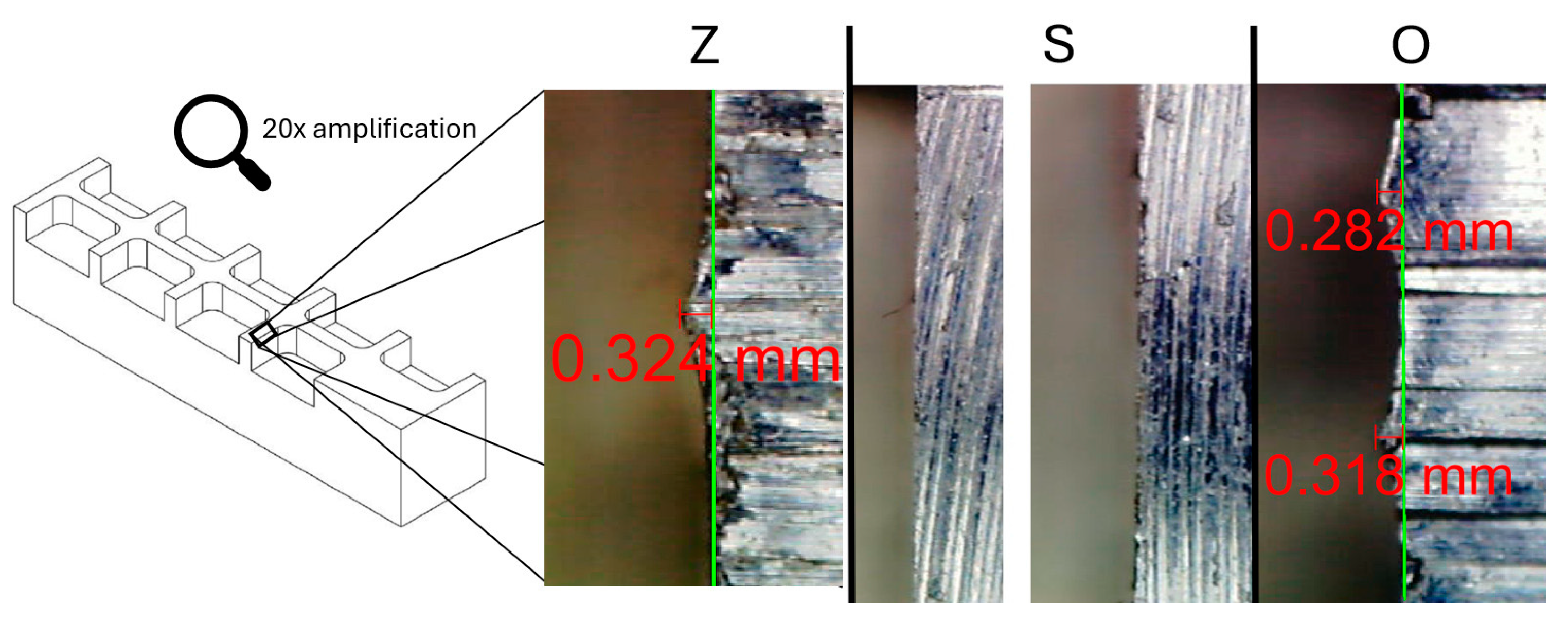
All pockets were evaluated using an electronic magnifier, enabling detailed observation of surfaces with roughness exceeding the resolution limits of the roughness tester. This method provided a more comprehensive assessment of surface characteristics. Table 9 displays the average R_z measurements obtained from the visual analysis for all pockets corresponding to each toolpath, while Figure 8 illustrates the specific locations where the data were acquired.

As presented in Figure 8, the S toolpath exhibited surface roughness levels below the threshold for visual detection. In contrast, certain Z and O samples displayed significantly higher roughness values, exceeding 300 µm, with average roughness measurements of 285 µm for the Z toolpath and 297 µm for the O toolpath as presented in

Table 10. Visual analysis roughness results (µm).

	Z	O
Perpendicular Lateral Average (Rz)	285.667	297.111
Parallel Lateral Average (Rz)	0.991	1.326
Times Higher	288.261	224.065

.

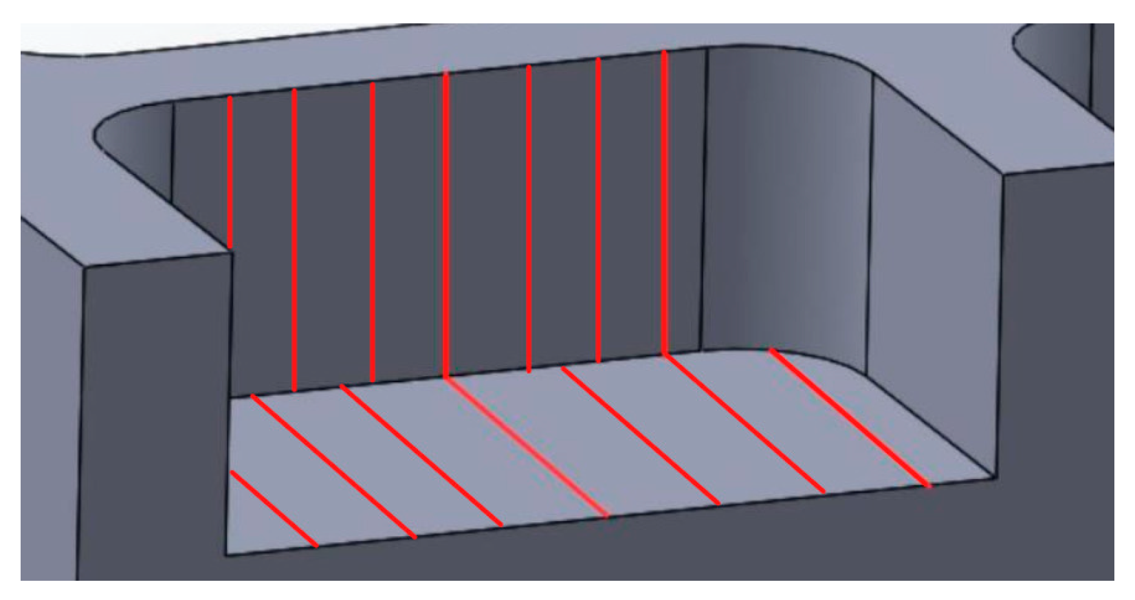
This phenomenon is attributed to the characteristics of the toolpath strategy. As illustrated in Figure 5, the O and Z toolpaths generate a radius difference along the pocket walls where the tool passes perpendicularly to the surface. This occurs due to the combination of the tool diameter and displacement between successive tool passes, leading to the formation of ridge-like peaks, as shown in Figure 5. Table 10 quantifies the disparity between the parallel and perpendicular pocket walls, revealing that the maximum roughness difference between these orientations ranges from 220 to 290 times, a variation that is far from negligible. To mitigate this effect, an additional finishing pass along the perpendicular walls is required, increasing machining time and reducing process efficiency, which contradicts the intended productivity gains of pocket milling cycles.

3.5. Performance Evaluation

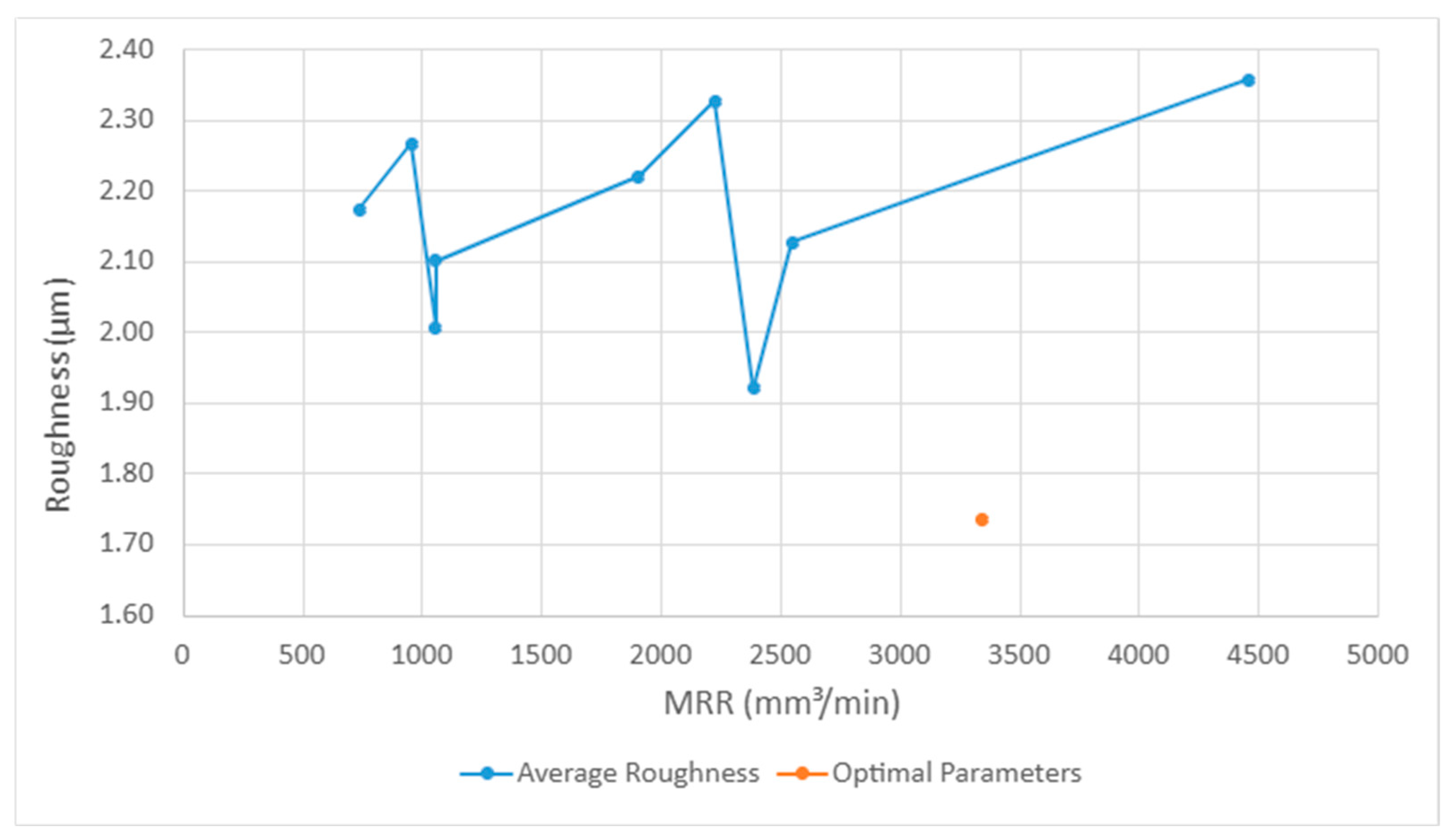
The cost of the CNC machining process is typically associated with the Material Removal Rate (MRR). In general, higher productivity corresponds to lower operational costs. Figure 9 illustrates the relationship between surface quality and productivity, revealing that, on average, an increase in MRR, particularly beyond 2400 mm³/min, is associated with a decline in surface quality. This occurs as the cutting speed remains constant beyond this point, leading to increased cutting forces. However, by applying the optimal parameters identified through Grey Relational Analysis, represented by the orange marker (Ra = 1.73 μm and 3342.36 mm³/min), it was possible to achieve a lower surface roughness while maintaining a high MRR, thus overcoming the typical trade-off between cost and quality.

4. Conclusions

This study demonstrated that integrating statistical techniques such as the Taguchi method, Grey Relational Analysis (GRA), and ANOVA enables the efficient optimization of milling parameters, enhancing both surface quality and productivity.

The results indicated that cutting speed was the most influential parameter in reducing surface roughness for the Zig-Zag and Parallel Spiral toolpaths, whereas axial penetration had a greater impact in the One-Way toolpath, particularly in maximizing material removal rate. Regarding Grey Relational Analysis, the Parallel Spiral toolpath emerged as the most balanced approach, with the V_c = 150 m/min, f_z = 0.025 mm/tooth, and a_p = 1.0 mm (A3-B3-C1) configuration effectively meeting both surface quality and productivity requirements, making it the most favourable solution for practical applications. It achieves an optimal equilibrium between cost efficiency and product quality, thereby establishing a balanced framework conducive to industrial implementation.

References

1. Benardos, P.; Vosniakos, G.C. Predicting surface roughness in machining: A review. Int. J. Mach. Tools Manuf. 2003, 43, 833–844. [Google Scholar] [CrossRef]
2. Trent, E.M.; Wright, P.K. Metal Cutting; Butterworth-Heinemann: Oxford, UK, 2000; ISBN 978-0-7506-7069-2. [Google Scholar]
3. Wang, M.-Y.; Chang, H.-Y. Experimental study of surface roughness in slot end milling al2014-t6. Int. J. Mach. Tools Manuf. 2004, 44, 51–57. [Google Scholar] [CrossRef]
4. Puertas-Arbizu, I.; Luis-Pérez, C.J. Surface roughness prediction by factorial design of experiments in turning processes. J. Mater. Process. Technol. 2003, 143, 390–396. [Google Scholar] [CrossRef]
5. Yang, W.H.; Tarng, Y. Design optimization of cutting parameters for turning operations based on the taguchi method. J. Mater. Process. Technol. 1998, 84, 122–129. [Google Scholar] [CrossRef]
6. Zhang, J.Z.; Chen, J.C.; Kirby, E.D. Surface roughness optimization in an end-milling operation using the taguchi design method. J. Mater. Process. Technol. 2007, 184, 233–239. [Google Scholar] [CrossRef]
7. Balaji, M.; Rao, K.V.; Rao, N.M.; Murthy, B. Optimization of drilling parameters for drilling of ti-6al-4v based on surface roughness, flank wear and drill vibration. Measurement 2018, 114, 332–339. [Google Scholar] [CrossRef]
8. Davim, J. A note on the determination of optimal cutting conditions for surface finish obtained in turning using design of ex-periments. J. Mater. Process. Technol. 2001, 116, 305–308. [Google Scholar] [CrossRef]
9. Nalbant, M.; Gökkaya, H.; Sur, G. Application of taguchi method in the optimization of cutting parameters for surface roughness in turning. Mater. Des. 2007, 28, 1379–1385. [Google Scholar] [CrossRef]
10. Wojciechowski, S.; Maruda, R.W.; Barrans, S.M.; Niesłony, P.; Królczyk, G.M. Optimisation of machining parameters during ball end milling of hardened steel with various surface inclinations. Measurement 2017, 111, 18–28. [Google Scholar] [CrossRef]
11. Wojciechowski, S.; Mrozek, K. Mechanical and technological aspects of micro ball end milling with various tool inclinations. Int. J. Mech. Sci. 2017, 134, 424–435. [Google Scholar] [CrossRef]
12. Wojciechowski, S.; Maruda, R.W.; Krolczyk, G.M.; Niesłony, P. Application of signal to noise ratio and grey relational analysis to minimize forces and vibrations during precise ball end milling. Precis. Eng. 2018, 51, 582–596. [Google Scholar] [CrossRef]
13. Lazoglu, I.; Manav, C.; Murtezaoglu, Y. Tool path optimization for free form surface machining. CIRP Ann. 2009, 58, 101–104. [Google Scholar] [CrossRef]
14. Zhou, J.; Ren, J.; Yao, C. Multi-objective optimization of multi-axis ball-end milling inconel 718 via grey relational analysis coupled with rbf neural network and pso algorithm. Measurement 2017, 102, 271–285. [Google Scholar] [CrossRef]
15. Abdulrazaq, M.M.; Jaber, A.S.; Hammood, A.S.; Abdulameer, A.G. Optimization of Machining Parameters for MRR and Surface Roughness for 7024 AL-alloy in Pocket Milling Process. Assoc. Arab. Univ. J. Eng. Sci. 2019, 26, 10–16. [Google Scholar] [CrossRef]
16. Upadrashta, A.; Saravanan, S.; Annamalai, A.R. Experimental Study on Dry Milling of Stir-Casted and Heat-Treated Mg-Gd-Y-Er Alloy Using TOPSIS. J. Manuf. Mater. Process. 2024, 8, 205. [Google Scholar] [CrossRef]
17. Felh, C.; Tesfom, F.; Varga, G. ANOVA Analysis and L9Taguchi Design for Examination of Flat Slide Burnishing of Unalloyed Structural Carbon Steel. J. Manuf. Mater. Process. 2023, 7, 136. [Google Scholar] [CrossRef]
18. Ross, P.J. Taguchi Techniques for Quality Engineering: Loss Function, Orthogonal Experiments, Parameter and Tolerance Design; McGraw-Hill: New York, NY, USA, 1988. [Google Scholar]
19. Ribeiro, J.; Lopes, H.; Queijo, L.; Figueiredo, D. Optimization of cutting parameters to minimize the surface roughness in the end milling process using the taguchi method. Period. Polytech. Mech. Eng. 2017, 61, 30–35. [Google Scholar] [CrossRef]
20. Lu, H.; Chang, C.; Hwang, N.; Chung, C. Grey relational analysis coupled with principal component analysis for optimization design of the cutting parameters in high-speed end milling. J. Mater. Process. Technol. 2009, 209, 3808–3817. [Google Scholar] [CrossRef]
21. Metalthaga. Technical Table—ALUMINUM ALLOY 5083-H111. 2019. Available online: https://metalthaga.com.br/wp-content/uploads/2019/09/liga-de-aluminio-5083-h111.pdf (accessed on 6 January 2024).
22. Starkey, C.V. Engineering Design Decisions; E. Arnold: London, UK, 1992. [Google Scholar]
23. Cimbala, J.M. Taguchi Orthogonal Arrays; Pennsylvania State University: University Park, PA, USA, 2014; pp. 1–3. [Google Scholar]
24. Hamzaçebi, C.; Li, P.; Pereira, P.A.R.; Navas, H. Taguchi method as a robust design tool. In Quality Control: Intelligent Manufacturing, Robust Design and Charts; IntechOpen: London, UK, 2020; pp. 1–19. [Google Scholar]
25. Julong, D. Introduction to grey system theory. J. Grey Syst. 1989, 1, 1–24. [Google Scholar]
26. Gau, H.; Hsieh, C.; Liu, C. Application of grey correlation method to evaluate potential groundwater recharge sites. Stoch. Environ. Res. Risk Assess. 2006, 20, 407–421. [Google Scholar] [CrossRef]
27. Liu, S.; Lin, Y. Grey Systems; Springer: Berlin/Heidelberg, Germany, 2010. [Google Scholar]
Figure 1. Study flowchart.
Jmmp 09 00148 g001
Figure 2. Tool paths.
Jmmp 09 00148 g002
Figure 3. CNC machine with milled sample.
Jmmp 09 00148 g003
Figure 4. Zig-Zag milled pockets.
Jmmp 09 00148 g004
Figure 5. Parallel Spiral milled pockets.
Jmmp 09 00148 g005
Figure 6. One-Way milled pockets.
Jmmp 09 00148 g006
Figure 7. Surface measurements.
Jmmp 09 00148 g007
Figure 8. Visual analysis.
Jmmp 09 00148 g008
Figure 9. Roughness versus MRR.
Jmmp 09 00148 g009