Detection of Release Fabric Defects in Fiber-Reinforced Composites Using Through-Transmission Ultrasound

Abstract

The detection of foreign material residues in fiber-reinforced composites (FRCs) is crucial, as such residues weaken the structural performance, especially when the acoustic impedance of the foreign material closely matches that of the composite material. To date, no methodology has been developed to improve the detection of such defects with similar acoustic impedance in the received signal without using echo-mode techniques. Release fabric was chosen because it is used in the fabrication of FRCs as a consumable, which must be removed after curing. An accidental residue of release fabric presents a significant challenge in detecting it within FRC laminates using through-transmission ultrasound (TTU) since its acoustic properties closely resemble the surrounding composite material, resulting in minimal impact on the transmitted signal and preventing accurate defect detection due to the lack of time-of-flight measurements. This paper leverages a novel threshold classifier to improve the detection of release fabric with through-transmission ultrasound (TTU), an inspection technique that operates without echo mode. Ultimately, this novel threshold classifier improves TTU inspection by offering greater sensitivity and detectability compared to conventional attenuation-based methods, particularly in the absence of echo mode and time-of-flight measurements. Future research will aim to investigate additional physical factors and deep learning approaches to further advance the TTU inspection method.

1. Introduction

Fiber-reinforced composite (FRC) laminates combine fibrous materials as reinforcement within a polymer matrix, followed by a curing process. These laminates are constructed from individual layers, called laminae, stacked together at various angles to form a multi-layered laminate structure [1]. FRC laminates are low-density combinations that provide improved structural performances, such as high specific strength, stiffness, fracture toughness, fatigue strength, and durability [1,2,3,4]. In conjunction, FRC laminates have a high strength-to-weight ratio, contributing to weight reduction, resulting in lower fuel consumption and overall operating expenses [1,5]. FRC laminates can be tailored toward specific applications based on loading conditions in which fibers are aligned to carry the required loads and deformations [2,5,6]. FRC laminates are very popular for high-volume processes across numerous industries [1,7]. Over 50 percent of next-generation commercial aircraft will include some FRC laminate, with percentages increasing for military applications [8]. FRC laminates can be tailored to include various geometric configurations, offering many advantages such as improved performance and functionality. Moreover, FRC laminates can be tailored to provide specific benefits to other factors and provide extended research opportunities to reduce manufacturing processing steps, weight, and time to improve part quality, providing a more straightforward, cost-effective product. FRC laminate manufacturing processes vary slightly based on method—wet layup, prepreg lamination, filament winding, pultrusion, and resin transfer molding (RTM) [9]. The manufacturing process of FRC laminates involves using materials such as bagging film, breather/bleeder cloth, parting film, release fabric, and wire systems, which are essential during fabrication but are not intended to remain in the final product [10]. Materials unintentionally left inside the final product are classified as foreign materials. These foreign materials can lead to delamination, where the layers (plies) of the composite separate, a critical defect that can compromise the structural integrity and potentially cause catastrophic failure [11].

Release fabric, or peel ply, is a consumable material used in FRC laminate fabrication and removed after curing. As it remains within the laminate, the release fabric must be detectable using nondestructive inspection (NDI) techniques, such as through-transmission ultrasound (TTU), which uses two opposing sensors to send and receive signals without relying on echo modes. In TTU, variations in amplitude between transmitted and received sound waves can indicate the presence of defects. These defects scatter, reflect, or absorb sound energy due to differences in acoustic impedance, reducing the amplitude of the transmitted signal as it is received. There are no echoes in the received signal. The acoustic properties of the release fabric can resemble the surrounding composite material. This resemblance provides minimal impact on the transmitted signal, resulting in reduced defect detection without the use of echo mode and time-of-flight measurements, and poses a challenge for accurate defect detection, as the subtle variations in the signal may be masked by noise or other interferences. Therefore, advanced signal processing techniques and statistical methods are crucial for improving the defect detection of release fabric in FRC laminates.

This paper leverages a novel threshold classifier to improve the detection of release fabric with through-transmission ultrasound (TTU), an inspection technique that operates without echo mode. Many real-world inspection scenarios may not permit ultrasonic inspection with echo mode due to constraints like complex geometries, high-attenuation materials, and the need for precise transducer alignment. TTU is better suited for these scenarios but faces challenges in detecting defects with low attenuation contrast, particularly when the defect’s acoustic impedance closely matches that of the surrounding material. To address this challenge, TTU signals from release fabric embedded in an FRC laminate were compared to baseline regions without release fabric. Both signal types were transformed into the frequency domain, and the root mean square (RMS) of the waveform values was calculated to improve contrast. Confidence intervals (CIs) were applied to establish an initial threshold, and a novel threshold classifier was developed by significantly improving the contrast between the baseline and defect signals. To date, no such method has been developed to effectively detect defects with similar acoustic impedance to the surrounding material, meaning this work yields a novel contribution in the field.

2. Background

2.1. Ultrasonic Inspection Methods for FRC Laminates

Many factors, such as the material inspected, manufacturing processes, defect type and location, part and defect geometry, and inspection requirements, influence the failure to detect subsurface defects. NDI processes are developed and implemented as a quality control measure to detect and locate defects such as foreign material to ensure product integrity and safety. Ultrasound is one such method, where sound energy is transmitted as a mechanical strain wave that alternates at ultrasonic frequencies. The basic principles of ultrasound rely on the ability of solid materials to propagate these strain waves, which are influenced by the material microstructure and properties [12]. Acoustic properties determine how materials respond to strain waves, with any deviations from a homogeneous structure, such as changes in material or geometry, altering the signal. A piezoelectric transducer introduces longitudinal strain waves into FRC laminates and converts electrical signals into mechanical energy and vice versa. The piezoelectric grain structure is aligned to induce an applied voltage (V±) producing strain displacement (Δ), as shown in Figure 1a. As particles are displaced, elastic oscillations produce longitudinal wave propagation through the thickness of the test piece at a specific wavelength (λ), as shown in Figure 1b. The transducer can be tailored into complex shapes for improved focusing and performance [13]. Ultrasound techniques are frequently utilized to characterize damage to microstructural features and elastic constants in FRC laminates [14,15,16]. Two main ultrasound techniques are used for volumetric inspection of FRC laminates: pulse-echo ultrasound (PEU) and through-transmission ultrasound (TTU). These techniques are illustrated in Figure 2 and Figure 3, respectively.

PEU is performed using a single transducer that transmits and receives strain waves from one surface of the material being inspected, as shown in Figure 2. The transducer emits a strain wave and receives the subsequent reflected strain wave as an echo over time. Reflections occur at material interfaces, such as the front and back surfaces, or where there are changes in the geometry, such as the presence of a defect. Due to the nature of strain wave propagation, these reflections are doubled. PEU determines the depth and location of these reflections by measuring the time-of-flight component in echo mode. An acquisition gate is set at a specific threshold, determined using a reference standard to capture echo reflections that exceed the threshold. Figure 2a illustrates the front and back surface echo reflections, the acquisition gate, and a no-defect echo reflection, while Figure 2b illustrates the same but with a defect echo reflection present and a reduced back surface echo reflection. The ability to detect foreign materials with similar acoustic impedance is discrete using echo mode, as the time-of-flight measurement allows for precise identification of defects, making them easier to detect than when using TTU. PEU is an industry standard for detecting subsurface defects and determining the depth of their distribution in FRC laminates [17,18,19,20,21].

TTU pre-dates PEU and is performed by using one transducer to transmit the strain wave and a second to receive the strain wave on opposing surfaces of the material inspected [22]. Through-transmission ultrasound (TTU) is widely used to detect subsurface defects in various materials by analyzing how sound energy propagates through attenuative media. Like pulse-echo ultrasound (PEU), defects in the material can scatter, reflect, or absorb sound energy, causing attenuation of the transmitted signal. However, unlike PEU, where the strain wave reflects off the material boundary interface and creates an echo, TTU operates by transmitting the strain wave through the material once. As a result, no echo is produced, and detection relies solely on the reduction in signal amplitude. Since TTU does not measure time of flight, it cannot determine the depth of a defect [23]. Instead, detectability is based on comparing the attenuation of the received signal to the baseline as a reference and then establishing a threshold for detectability. However, this method does not provide in-depth information [24]. Figure 3a illustrates the received peak signal exceeding the acquisition gate, established as the threshold, indicating no defect. In contrast, Figure 3b illustrates the received peak signal that is attenuated and falling below the acquisition gate threshold, which indicates a defect. This acquisition gate is established as the threshold identifier to distinguish between no defect and defect based on the received signal amplitude in TTU mode.

While PEU is generally more reliable for defect detection due to its ability to measure time of flight, many real-world inspection scenarios may not permit PEU due to constraints like complex geometries, high-attenuation materials, and the need for precise transducer alignment. TTU is better suited for these scenarios but faces challenges in detecting defects with low attenuation contrast, particularly when the defect’s acoustic impedance closely matches that of the surrounding material. This limitation underscores the need for improved detection methodologies. To address this challenge, this study introduces an advanced signal processing and statistical approach that enhances TTU’s ability to identify release fabric defects. The novel threshold classifier compensates for TTU’s typical limitations, improving its viability for detecting such defects and expanding its applicability as a machine learning model for TTU.

2.2. Principles of Acoustic Impedance

Defect detection depends on quantifying energy lost in strain wave intensity through the media (i.e., material). The material property on either side of the boundary interface is acoustic impedance—the measurement of opposition to strain wave propagation—resulting from compression pressure and density [25]. The acoustic impedance ($Z$) describes the resistance of strain wave propagation through the test component. The impedance is equal to the product of material density ($\rho )$ and speed of sound ($\nu )$, as shown in (1). The energy lost (or reflected) can be quantified using the reflection coefficient, which depends on the difference in acoustic impedance between the two media.

$$Z=\rho \nu$$

(1)

Acoustic strain waves are disrupted at boundaries of dissimilar acoustic impedance. The percentage of the reflected strain wave is determined by the reflection coefficient (R). The reflection coefficient is calculated as the ratio of reflected strain wave intensity (I_r) to incident strain wave intensity (I_i), as given by (2), where (Z₁) is the acoustic impedance of material one and (Z₂) is the acoustic impedance of material two.

$$R={\displaystyle \frac{I_r}{I_i}}={\left({\displaystyle \frac{Z_2-Z_1}{Z_2+Z_1}}\right)}^2$$

(2)

Conversely, the percentage of the strain wave that is transmitted is determined by the transmission coefficient (T). The transmission coefficient is calculated as the strain wave intensity of the transmitted beam (I_t) to the received strain wave intensity (I_r), as given by (3), where (Z₁) is the acoustic impedance of material one and (Z₂) is the acoustic impedance of material two.

$$T={\displaystyle \frac{I_t}{I_r}}={\displaystyle \frac{{4Z_{2}Z}_1}{(Z_2+Z_1{)}^2}}=1-R$$

(3)

The reflection and transmission coefficients resulting from interactions between water, an FRC laminate, and air are based on the acoustic properties of standard materials, such as those shown in Figure 4 [26]. The reflection coefficient from water to the FRC is 26.19%, while the reflection coefficient from the FRC to air is 99.93%, indicating a significant acoustic impedance mismatch between the FRC laminate and air.

2.3. Release Fabric Detection with Ulrasound

In manufacturing FRC laminates, several materials used during the process are not meant to remain in the final product and are, therefore, classified as foreign materials [27]. Since release fabric is a consumable material used to fabricate composite materials and can become foreign material within the laminate, it must be detected and reported through NDI methods. Its presence is critical to identify, as it can lead to catastrophic failure [26,28]. If any foreign materials are found to be undetectable, they are not permitted to remain in the manufacturing process. The detectability of release fabrics is, therefore, critical and can compromise the integrity of the final product.

Several strategies can be employed to improve the detection of foreign materials with ultrasound techniques [29,30,31]. PEU was determined to have the highest detection accuracy by determining the depth and location of reflections by measuring the time-of-flight component in echo mode, measuring the time it takes for the strain wave to travel through the material and back. Defects that do not cause significant amplitude changes can more often be detected due to minor time delays in the echo response [26,29,30]. While TTU was evaluated for detecting embedded foreign object inclusions within a composite, it was less effective than PEU [31]. TTU inspection is based on material acoustic properties and how sound energy propagates through the material and is attenuated at physical interfaces [22,32]. The difference in attenuation is determined by setting a threshold based on the signal attenuation below the acquisition gate threshold, which is established using a reference standard as the baseline. This is then compared to known defects to assess detectability [33]. The process effectively detects foreign materials with a significant difference in acoustic impedance, such as PTFE and other similar materials, which attenuate more than release fabrics. These materials can be easily identified due to their higher attenuation than the surrounding laminate [29,31]. In comparison, the acoustic impedance of both fiberglass and polyamide release fabrics closely matches that of FRC laminates.

Table 1. Acoustic properties of standard materials. Note: 1.0 inch = 25.4 mm; 1.0 lb = 0.454 kg.

Material	Density [lb/in3]	Sound Velocity [in/µsec]	Acoustic Impedance [lb/in2s]	Reflection Coefficient	Transmission Coefficient
Air	0.00004	0.025	1.11	99.93%	0.07%
FRC Laminate	0.05780	0.117	6762.60
Water	0.03610	0.061	2184.17	26.19%	73.81%
FRC Laminate	0.05780	0.117	6762.60
Fiberglass Release Fabric	0.04690	0.108	5065.20	2.06%	97.94%
FRC Laminate	0.05780	0.117	6762.60
Polyamide Release Fabric	0.04480	0.087	3897.60	7.22%	92.78%
FRC Laminate	0.05780	0.117	6762.60

presents the acoustic properties of selected standard materials, highlighting the similarity between two types of release fabric—fiberglass and polyamide—and FRC laminates. In this study, the FRC laminate standard was fabricated following industry specifications using BMS 8-276 carbon fiber tape combined with a toughened epoxy matrix. The FRP laminate standard was manufactured using an automated fiber placement process to ensure precision and repeatability. Each ply within the laminate is 0.008 inches (0.2 mm) thick. The layup follows a quasi-isotropic configuration, meaning that fiber orientations are distributed in-plane of the laminate and achieved by four primary orientations—0°, ±45°, and 90°, and arranged in a repeating sequence to maintain uniform mechanical properties in the in-plane direction.

The signal transmission between fiberglass and polyamide release fabric materials and FRC laminates is 97.94% and 92.78%, respectively. As a result, detecting release fabric with acoustic properties similar to FRC laminates is challenging, as minimal energy loss leads to minor differences in attenuation that are difficult to threshold. This study introduces a novel approach combining advanced signal processing techniques and statistical analysis to improve release fabric detection using TTU. TTU signals from release fabric embedded in an FRC laminate were compared to baseline regions without release fabric. Both signal types were transformed into the frequency domain, and the root mean square (RMS) of the waveform values was calculated to improve contrast. Confidence intervals (CIs) were applied to establish an initial threshold, and a novel threshold classifier was developed, significantly improving the contrast between the baseline and defect signals and improving the detection of release fabric in FRC laminates.

3. Materials and Methods

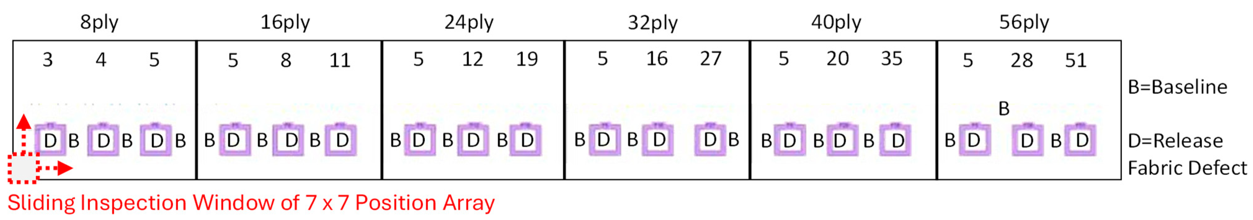
3.1. FRC Laminate Reference Standard

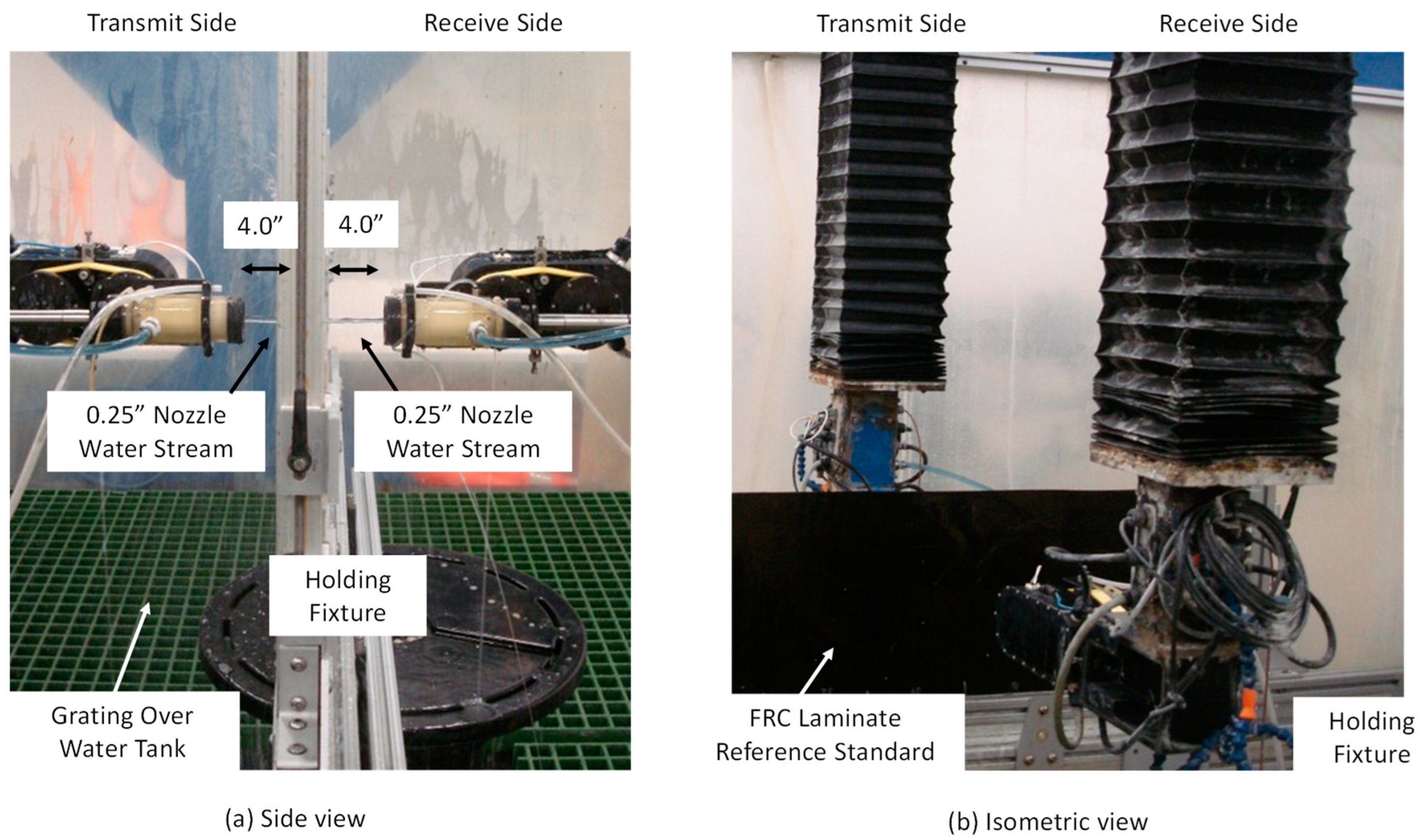
Due to the complexity introduced by multiple materials and stacking sequences, ultrasonic signals can become challenging to interpret [34]. As a result, a comparison method was employed using a reference standard. This standard comprised a pristine, undamaged section and controlled placements of embedded release fabric inserts (0.70 in × 0.70 in = 17.78 mm × 17.78 mm) to simulate foreign material residues. The reference standard was designed with multiple ply steps, each being 0.008 inches (0.2 mm) thick, with configurations of 8, 16, 24, 32, 40, and 56 plies. For reference,

Table 2. Release fabric defect matrix of the reference standard.

Standard Ply Step	Insert ID	Insert Type	Insert Area (inch2)	Ply Depth from Top Surface	Insert Location
8	8-3	Release Fabric	0.49	3	Near
	8-4		0.49	4	Mid
	8-5		0.49	5	Far
16	16-5		0.49	5	Near
	16-8		0.49	8	Mid
	16-11		0.49	11	Far
24	24-5		0.49	5	Near
	24-12		0.49	12	Mid
	24-19		0.49	19	Far
32	32-5		0.49	5	Near
	32-16		0.49	16	Mid
	32-27		0.49	27	Far
40	40-5		0.49	5	Near
	40-20		0.49	20	Mid
	40-35		0.49	35	Far
56	56-5		0.49	5	Near
	56-28		0.49	28	Mid
	56-51		0.49	51	Far

Note: 1.0 inch = 25.4 mm; 1 inch² = 645.16 mm².

is a release fabric defect matrix of the reference standard that identifies the ply step, insert identification, insert type, insert area as the geometry, ply depth from the top surface, and the insert location as the placement region.

The inserts are symmetrically aligned, as illustrated in Figure 5. Figure 5a is the cross-section view of the reference standard with release fabric inserts positioned near, mid, and far from the top. Figure 5b is the planar view indicating ply counts at each of the six steps, along with the size and location of release fabric inserts relative to the dimensions of each step. Additionally, it displays the overall length and width of the reference standard. Finally, the FRC laminate standard was fabricated following industry specifications using BMS 8-276 carbon fiber tape combined with a toughened epoxy matrix. The FRP laminate reference standard was manufactured using an automated fiber placement process to ensure precision and repeatability. The layup follows a quasi-isotropic configuration, meaning that fiber orientations are distributed in-plane of the laminate and achieved by four primary orientations—0°, ±45°, and 90°, and arranged in a repeating sequence to maintain uniform mechanical properties in the in-plane direction. The laminate was then cured in an autoclave at controlled temperature and pressure. The proceeding process was selected to replicate FRC laminate requirements manufactured to meet high-performance characteristics, ensuring the reference standard resembles real-world applications.

3.2. TTU Inspection

Figure 6 depicts the TTU inspection setup with the reference standard. Figure 6a shows a side view and Figure 6b an isometric view. The reference standard included additional pre-drilled holes intended for other research applications; however, these holes did not influence the TTU inspection results (not shown in Figure 6).

The reference standard was used to calibrate the ultrasonic equipment, with signals from the undamaged regions serving as the baseline for each thickness. For this study, a 5 MHz, 0.75-inch (19.05 mm)-diameter, 4.375-inch (111.13 mm) spherically focused transducer was selected to balance sensitivity, resolution, and attenuation based on the reference standard’s thickness and the sensitivity of the system in detecting release fabric inserts. The reference standard holding fixture was aligned perpendicular to the transmit and receive nozzles to ensure normality and optimal signal strength. A 4.00-inch (101.6 mm) standoff between each nozzle and the standard was set up to prevent interference with the fixture. Two 0.250-inch (6.35 mm) nozzles (one on each side) were chosen to enhance resolution while maintaining laminar water flow.

The reference standard was scanned using a scan grid of 0.08 × 0.08 inch² (2.03 × 2.03 mm²) and a sampling period of 0.02 microseconds. This sampling period was specifically identified to avoid aliasing errors caused by a low sampling rate. The data were collected and stored as a function of scan (m), index (n) position, and time (t). An acquisition gate was implemented to detect and isolate the maximum amplitude signal for each sampling period, measured in volts, represented in the amplitude scan (A-scan). The data were arranged in a 7 × 7 matrix array of 49 pixels, as the sample size. Accordingly, each pixel represents the position (m, n) and the corresponding maximum signal amplitude, displayed in a 2D map. The highest signal amplitude (V_high) was set to white and the lowest signal amplitude (V_low) to red using a color pallet, with 256 shades of gray gradient, for maximum contrast between the baseline and the release fabric defect. Figure 7a shows the A-scan at a position, Figure 7b the corresponding voltage-to-color mapping, and Figure 7c the resulting m x n position array as the sample.

Brighter colors indicate areas of the baseline, while darker colors are based on attenuation, highlighting areas with release fabric defects. The C-scan image color pallet was established using 256 shades of gray gradient. Figure 8 shows a standard defect map, illustrating the location of the baseline (B) and release fabric defect (D) patterns, with a total of 1764 data points. The sliding inspection window of the 7 × 7 position array in Figure 8 is used to collect TTU data, as depicted in Figure 7.

4. Results

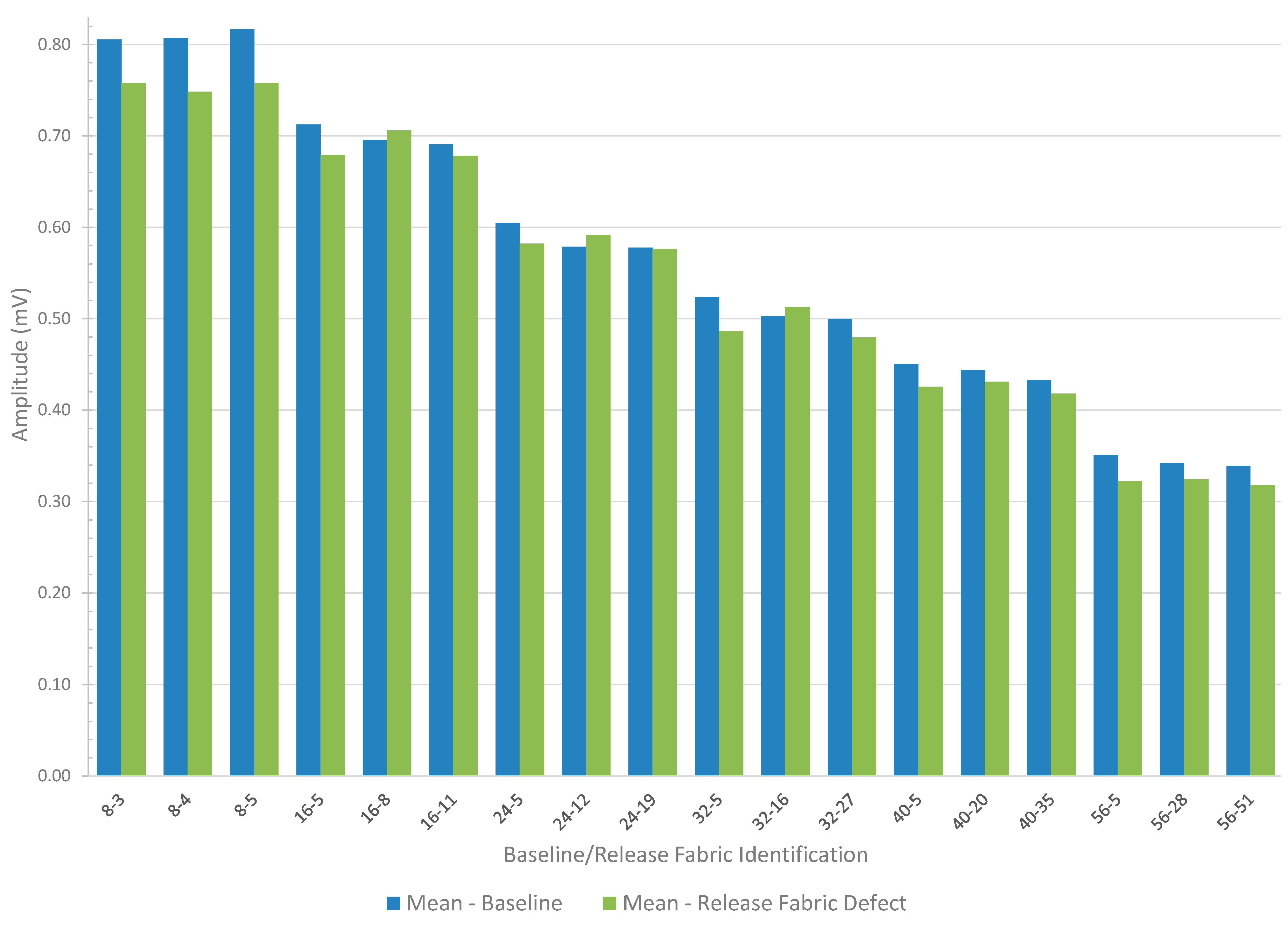
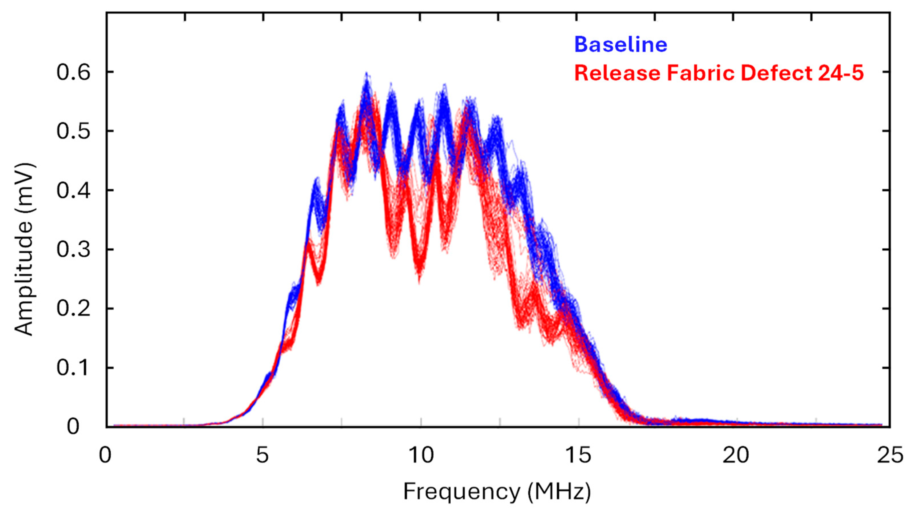
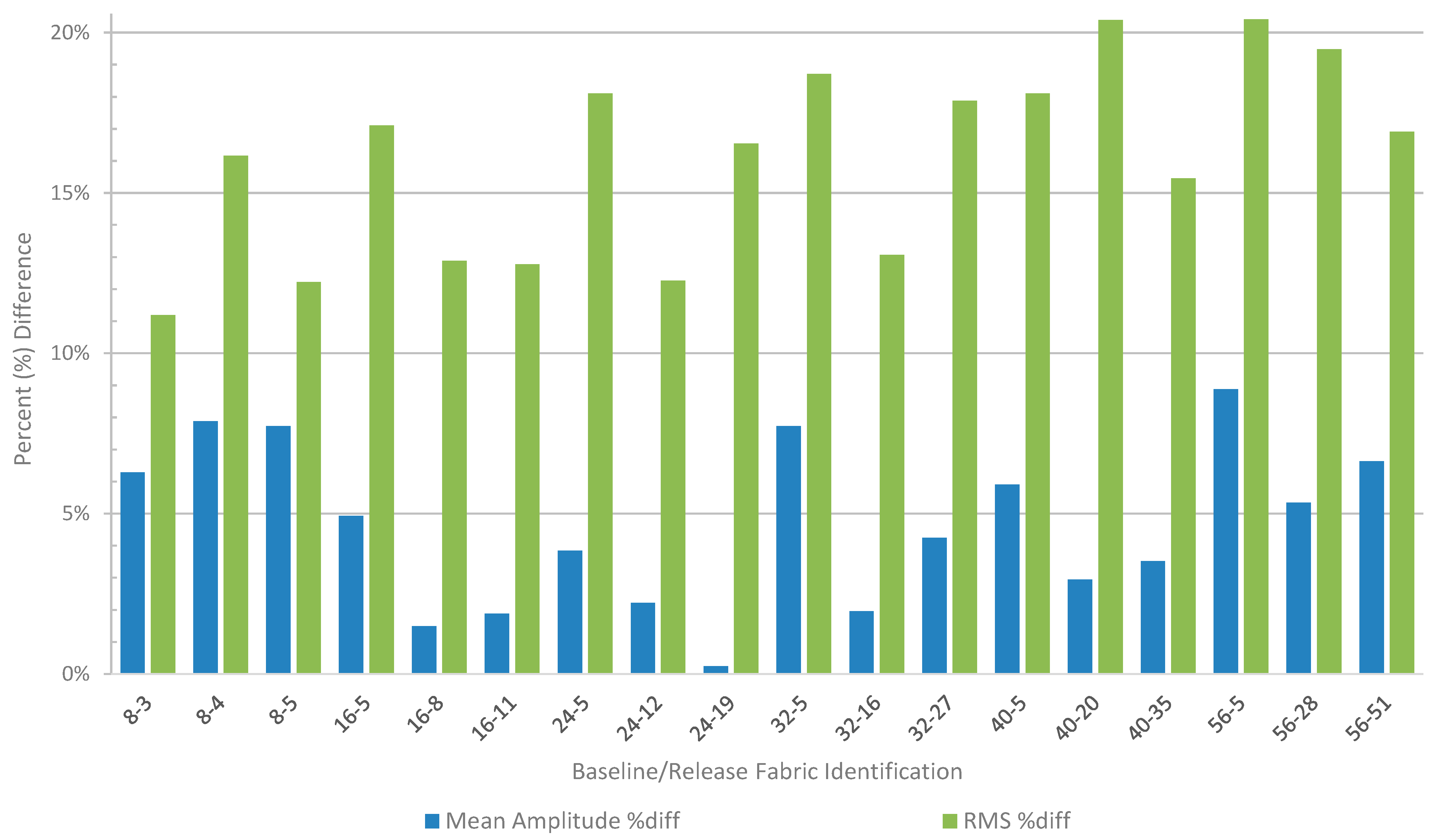
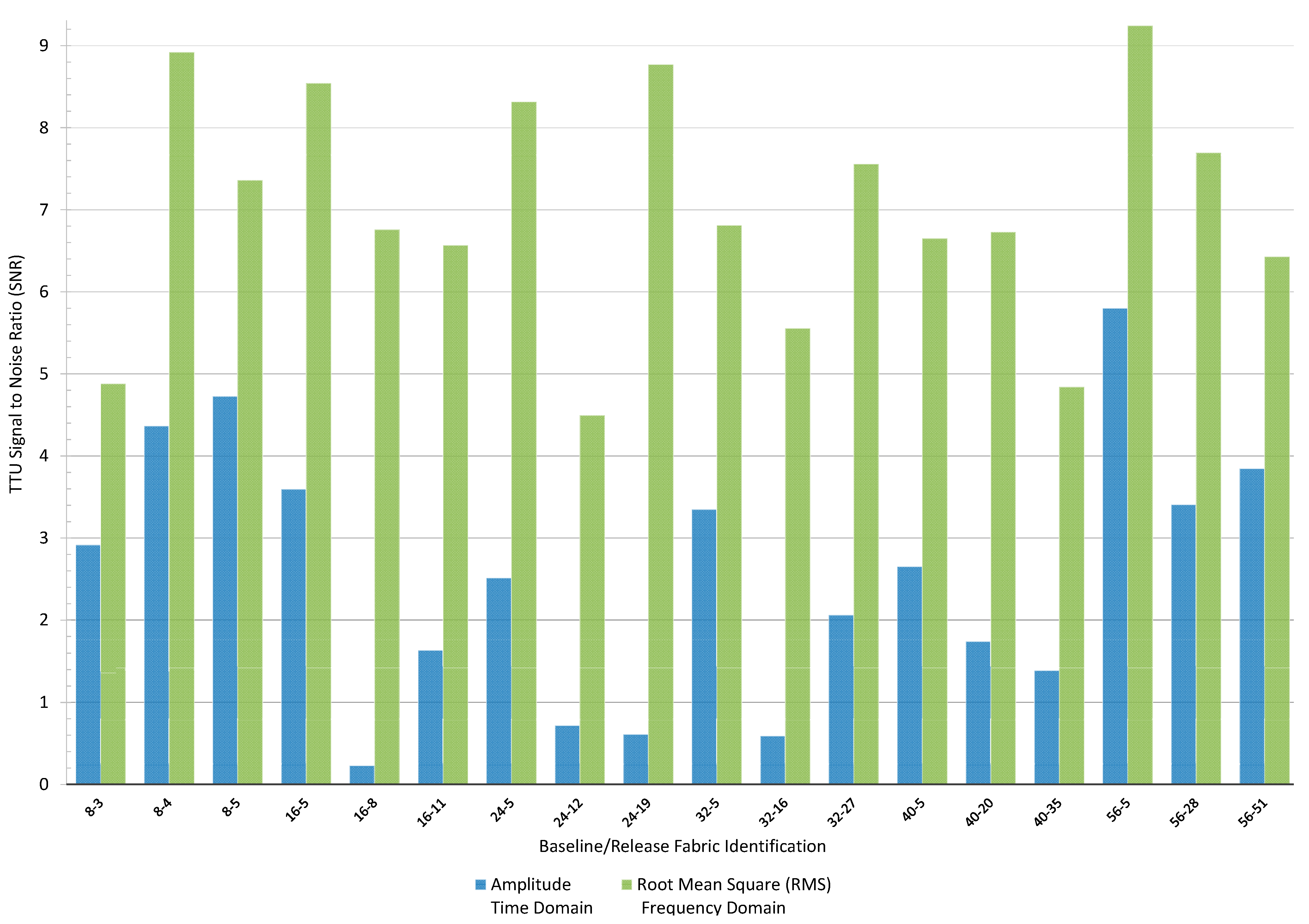
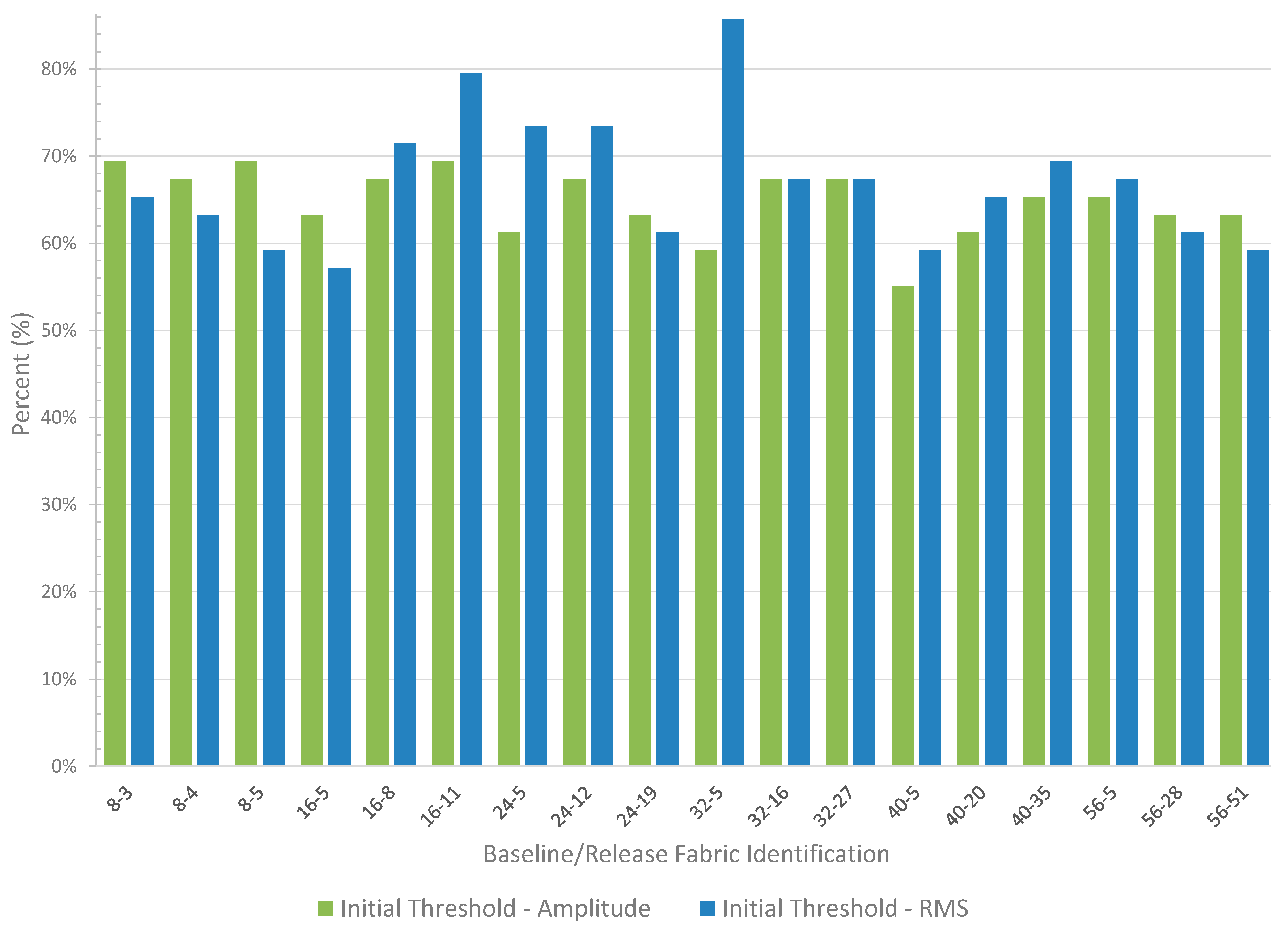
4.1. Preliminary Analysis

Ultrasonic signal analysis is complex due to the various reflections, transmission coefficients, and dispersion modes. These signals are reflected or dispersed at each physical boundary, such as interfaces of different acoustic impedance and defects that scatter, reflect, or absorb the sound energy, causing attenuation that affects the overall signal [34]. Several signal processing analysis tools derived from different domains are used to further evaluate various defects and materials, such as the time, frequency, and phase domains for PE or echo mode [14,35,36,37]. Industry-standard TTU evaluation methods monitor the received signal amplitude in the time domain based on attenuation, reported in volts (V), decibels (dB), or percent full-screen height (%FSH). In contrast, PE evaluation methods use echo mode to establish the time-of-flight component via peak-to-peak or threshold crossing methods [22,23], and enveloped signals [38].

Figure 9 shows unprocessed TTU amplitude results, comparing the amplitudes (measured in millivolts, mV) of the mean baseline and the mean release fabric defect in the time domain.

The data in Figure 9 represents each sample size comprising 49 pixels (as shown in Figure 7 and identified in Figure 8) across the different thicknesses of the reference standard detailed in Table 2. The average amplitude difference between the baseline and the release fabric defect is 0.021 mV, with attenuation increasing as the reference standard thickness grows. The percentage (%) difference was calculated to normalize the difference and account for attenuation, making it easier to observe the proportional change. The percentage difference between the mean baseline and the mean release fabric defect is 4.65%. This detailed analysis of minor amplitude variations highlights the difficulty of establishing a universal threshold to effectively differentiate between release fabric defects and the baseline using the TTU amplitude, particularly without echo mode.

The TTU signals were then processed, transforming them from the time domain to the frequency domain using the discrete Fourier transform (DFT) [39]. The frequency domain primarily highlights frequency components through the power density spectrum, which measures signal power as a function of frequency [40]. The discrete Fourier transform (DFT) is then related by (4), where $X_m$ is the DFT of $x\left[n\right]$, of length $N$ [41].

$${\sum }_{n=0}^{N-1}{\left|x\left[n\right]\right|}^2={\displaystyle \frac{1}{N}}{\sum }_{m=0}^{N-1}{\left|X\left[m\right]\right|}^2$$

(4)

For illustration, Figure 10 presents the post-processed TTU frequency spectrum, comparing the amplitude vs. the frequency for both the baseline and release fabric defect 24-5, as an example.

The values of the RMS relative to the signal are commonly used in signal processing techniques to measure the difference in magnitude of the varying signals by taking both the positive and negative components collectively. The use of the RMS is important for establishing a statistical estimate to describe the RMS deviation from zero, offering a measure of the signal magnitude [42,43]. The RMS provides a meaningful way to measure and compare the overall signal strength, particularly in ultrasonic testing, giving better insight into differences in signal amplitude, especially when variations between the baseline and defect are subtle [44]. The RMS can be identified in either the time domain (i.e., quantifying the magnitude of a signal over time) or the frequency domain (i.e., the magnitude of different frequency components of the signal) [41,45]. For a continuous signal, the RMS of a continuous-time signal $x\left(t\right)$ is a measure of the signal magnitude over time, defined by (5), where T₁ and T₂ are the start and the end of a time interval, x(t)² is the square of the signal at each point in time, and 1/(T₂ − T₁) normalizes the value by the time interval T.

$$x_{RMS}=\sqrt{{\displaystyle \frac{1}{T_2-T_1}}{\int }_{T_1}^{T_2}\left|x{\left(t\right)}^2\right|dt}$$

(5)

The RMS value of discrete-time samples ${\{x}_n\}$, where $n$ is the time index at each sample taken, is given as (6) [45].

$$x_{RMS}=\sqrt{{\displaystyle \frac{\left|x_0^2\right|+\left|x_1^2\right|+\dots +{\left|x_{N-1}\right|}^2}{N}}}=\sqrt{{\displaystyle \frac{1}{N}}{{\sum }_{n=0}^{N-1}\left|x_n\right|}^2},n=0,\dots ,N-1$$

(6)

The energy of the signal in terms of the average energy of the frequency spectrum is defined by Parseval’s theorem. The energy of the signal from the time domain, as discrete-time samples (N), is equivalent to the energy contained in discrete-frequency components ${\{X}_m\}$, where $m$ is the frequency index as given by (7) [39]. The RMS formulas are summarized by (8).

$$X_m={\sum }_{n=0}^{N-1}{x}_n{e}^{-2\pi inm/N},i=\sqrt{-1},m=0,\dots ,N-1$$

(7)

$$x_{RMS}=\sqrt{{\displaystyle \frac{1}{N}}{\sum }_{\mathrm{n}}{\left|x_n\right|}^2}=\sqrt{{\displaystyle \frac{1}{N^2}}{{\sum }_m\left|X_m\right|}^2}=\sqrt{{{\sum }_m\left|{\displaystyle \frac{X_m}{N}}\right|}^2}$$

(8)

The RMS was calculated from the frequency components of the TTU signal. Figure 11 illustrates the amplitude (mV) compared to the RMS values of the baseline and release fabric defect derived from these frequency components. The percentage (%) difference between the RMS of the baseline relative to the RMS of the release fabric defect is 16.09%.

The signal-to-noise ratio (SNR) is a key indicator of defect detectability. It is the most suitable method for quantifying defects using statistical approaches, thereby minimizing false positives and enhancing reliability [26]. An SNR of 3:1 is a common industry standard derived from the signal response of a defect as measured against a reference standard [46]. SNR values were calculated according to Equation (9); the mean value µ₂ (which accurately sizes the defect by ±25%) is subtracted from the background mean µ₁ (known good area adjacent to the defect) and then divided by the standard deviation σ₁ of the background [26].

$$SNR={\displaystyle \frac{{(\mu }_1-{\mu }_2)}{{\sigma }_1}}$$

(9)

Figure 12 illustrates the percentage difference between the mean amplitude and the RMS change in terms of the respective percentage differences. RMS processing leads to an 11.45% variation in magnitude relative to the mean amplitude, indicating an improvement.

Figure 13 illustrates the TTU SNR in the time domain and the RMS in the frequency domain. The RMS time domain yields an average SNR of 2.56, and the RMS frequency domain yields an SNR of 7.01. The SNR values indicate that the RMS frequency domain significantly improves defect detection compared to the time domain.

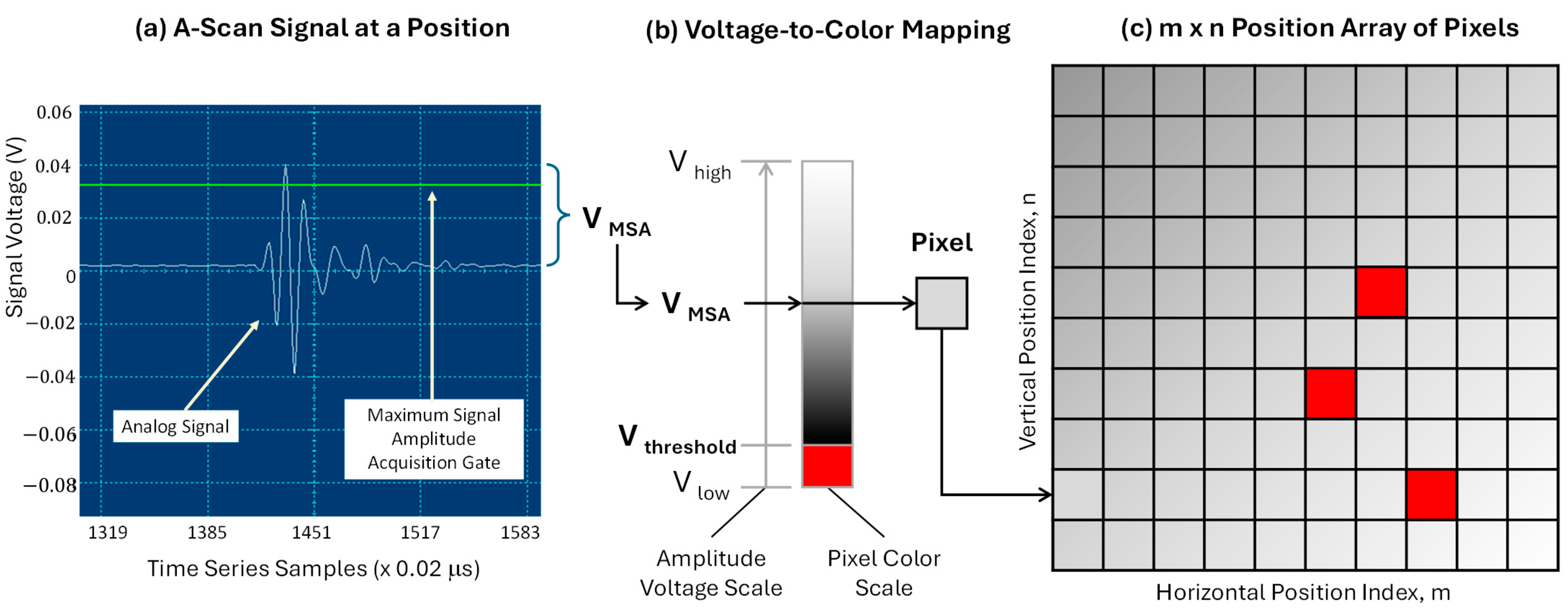
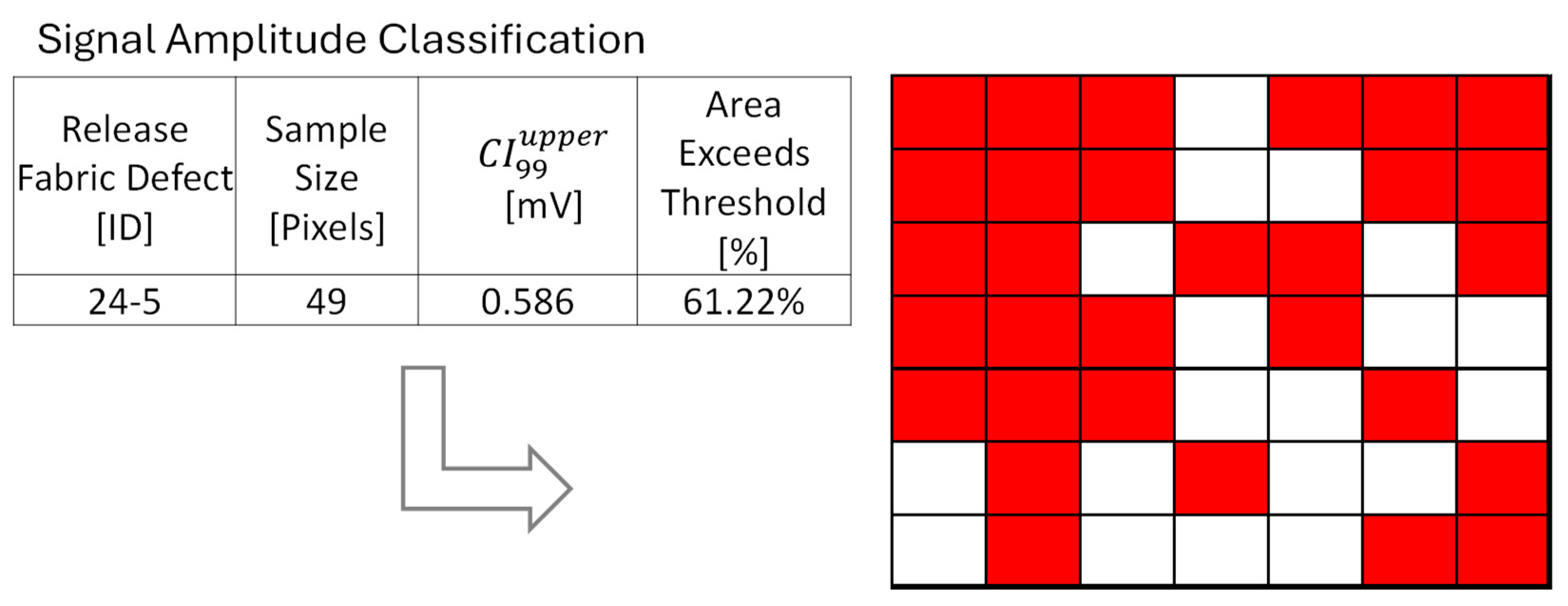
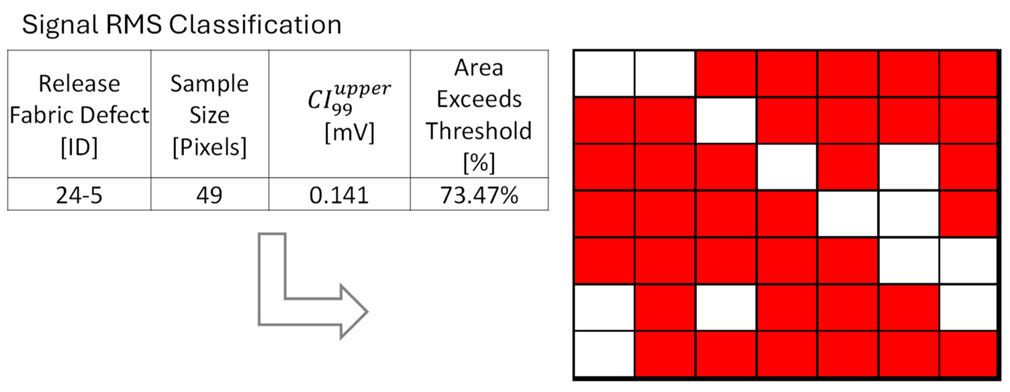
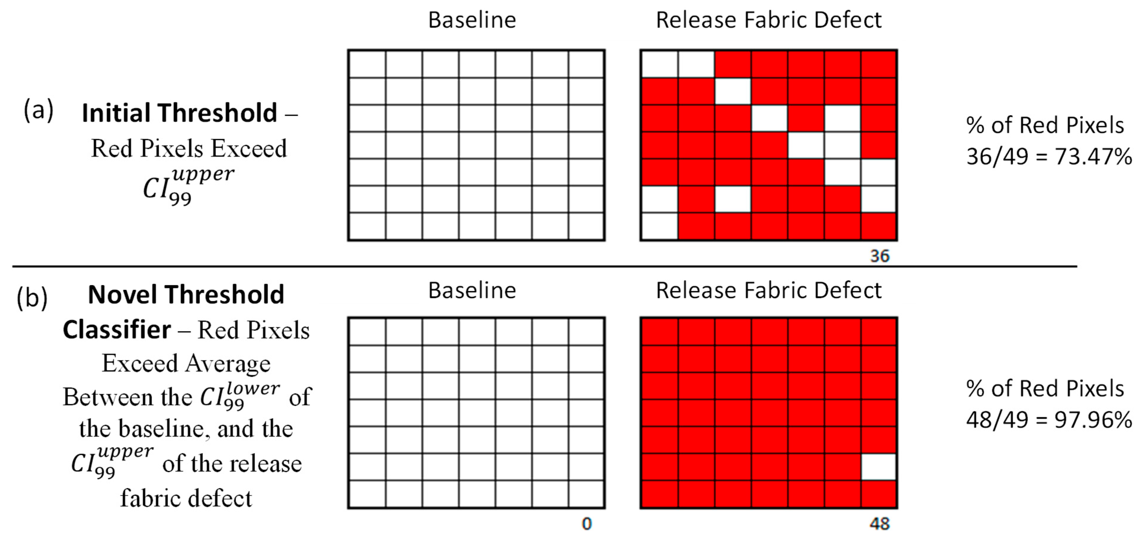
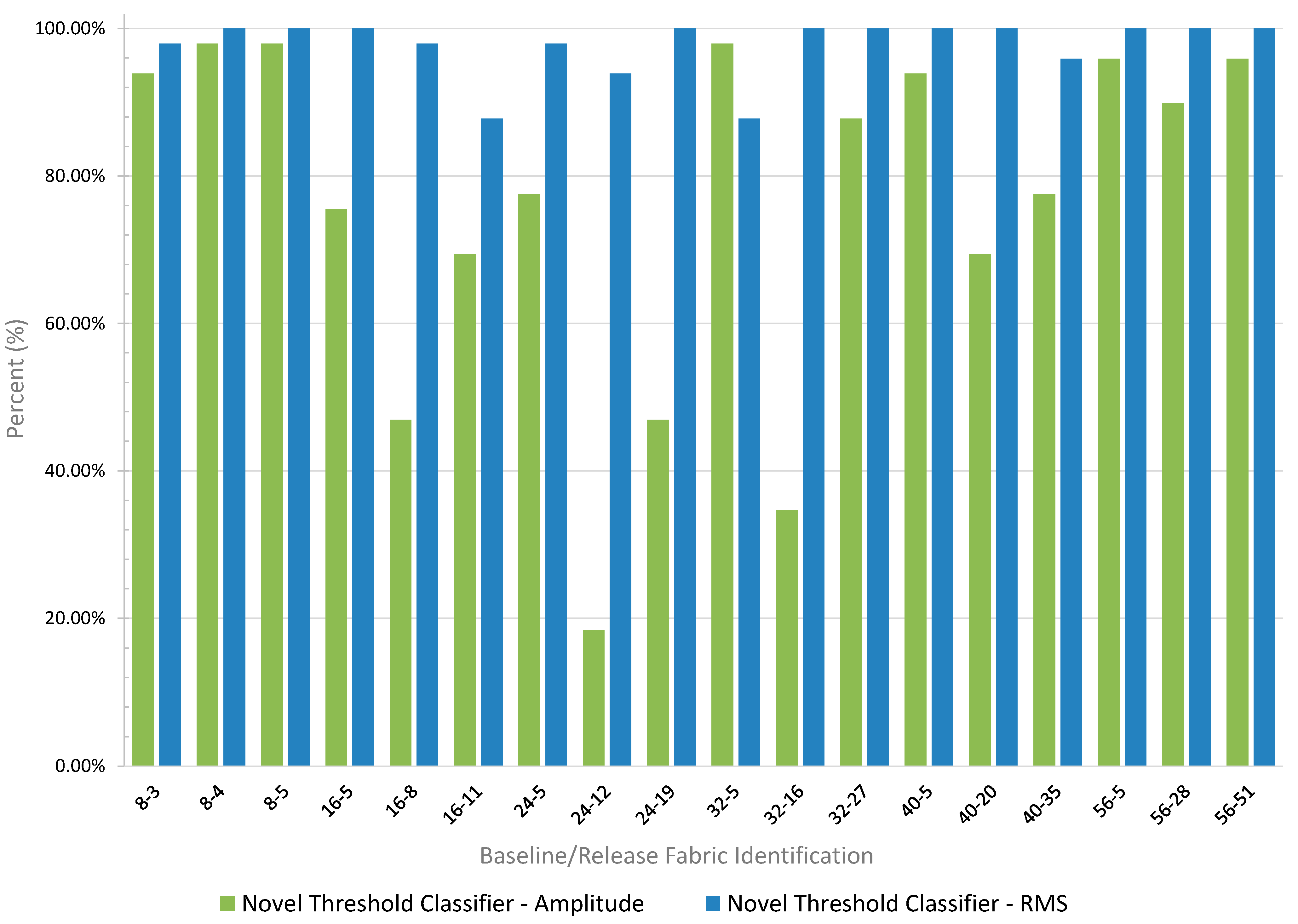
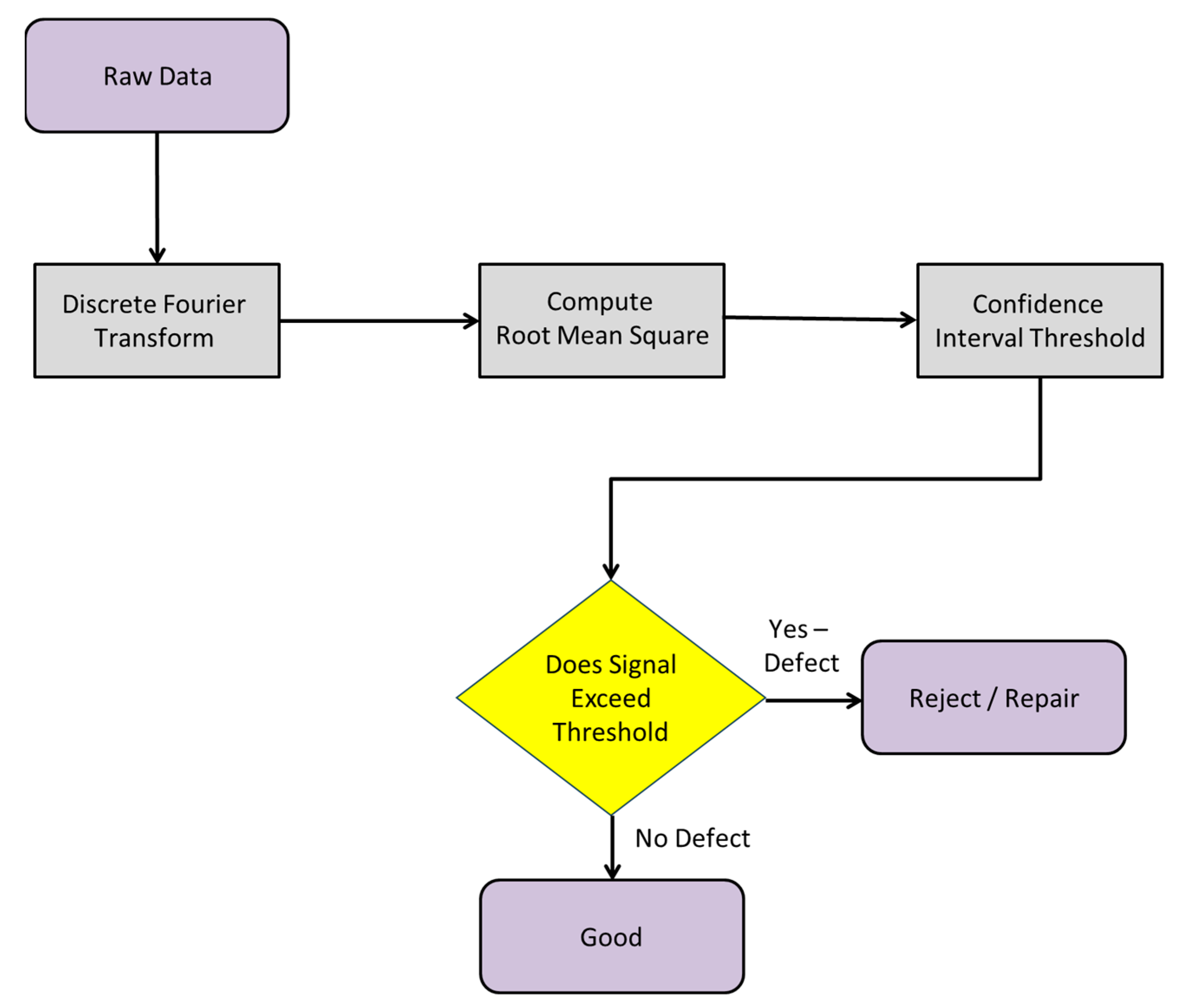
4.2. Threshold Classification

Confidence intervals (CIs) were introduced and applied as an initial threshold to improve detection between the amplitude of the baseline and the release fabric defect for TTU. Subsequently, a novel threshold classifier was developed, which significantly improved the contrast between the two conditions, optimizing the detection of release fabric in fiber-reinforced composites.

First, the initial threshold establishes a population parameter that more effectively quantifies the difference’s detectability for TTU. Equation (10) was used to establish the CI for both the amplitude and RMS, where the sample mean is the confidence level value, s is the sample standard deviation, and n is the sample size (49 pixels).

$$CI=\overline{x}\pm z{\displaystyle \frac{s}{\sqrt{n}}}$$

(10)

The initial thresholds for amplitude and RMS were established to prevent false negatives in TTU detection. They were set to the upper limit of the 99% confidence interval (${CI}_{99}^{upper}$) from each sample set of 49 pixels, as shown in Figure 7 and identified in Figure 8, across the different thicknesses of the reference standard specified in Table 2.

Figure 14 illustrates the initial amplitude ${CI}_{99}^{upper}$ threshold for release fabric defect 24-5, as an example. Figure 14 shows the amplitude summary table of defect 24-5, where the ${CI}_{99}^{upper}$ threshold is 0.586 mV, and the resulting pixel area that exceeds the ${CI}_{99}^{upper}$ is 61.22%, indicated by red. Figure 15 illustrates the initial RMS ${CI}_{99}^{upper}$ threshold for release fabric defect 24-5, as an example. Figure 15 shows the RMS summary table of defect 24-5, where the ${CI}_{99}^{upper}$ threshold is 0.141 mV, and the resulting pixel area that exceeds the ${CI}_{99}^{upper}$ is 73.47%, indicated by red.

Figure 16 shows the results of the initial threshold classification. The results reveal that 64.74% of the pixels exceed the threshold for amplitude, and 67.01% exceed the threshold for RMS, indicating improved detectability with RMS values.

A novel threshold classifier was developed to improve the detection of release fabric defects, significantly improving the contrast between the baseline and release fabric defect conditions for each sample size comprising 49 pixels (as shown in Figure 7 and identified in Figure 8) across the different thicknesses of the reference standard detailed in Table 2. This classifier maximizes the percentage of true positive pixels while minimizing false positives. It was established by leveraging the average between the ${CI}_{99}^{lower}$ of the baseline and the ${CI}_{99}^{upper}$ of the release fabric defect, as shown in Equation (11).

$$Average={\displaystyle \frac{X+Y}{2}}$$

(11)

where

• X is the ${CI}_{99}^{lower}$ value from the sample size (e.g., 49 pixels) of the baseline;
• Y is the ${CI}_{99}^{upper}$ value from the sample size (e.g., 49 pixels) of the release fabric defect.

Figure 17 compares the initial threshold and the novel threshold classifier results for defect 24-5, as an example. Figure 17a shows the initial threshold, where the red pixels represent those exceeding the 73.47% threshold. Figure 17b illustrates the results from the novel threshold classifier based on the calculated average between the ${CI}_{99}^{lower}$ of the baseline and the ${CI}_{99}^{upper}$ of the release fabric defect (as shown in Equation (11)). The red pixels represent those that exceed the novel threshold, where 97.96% represent the release fabric defect.

Figure 18 compares the amplitude data and the RMS data for the novel threshold classifier. The results indicate that 75.96% of the pixels exceed the amplitude threshold, whereas 97.73% exceed the RMS threshold, demonstrating a significant improvement in release fabric detection using the RMS classifier.

Figure 19 illustrates a flowchart that outlines the process from raw data acquisition to the final determination of defect presence or absence based on whether the signal exceeds the novel threshold. This classifier was specifically developed to improve the detection of release fabric defects in fiber-reinforced composites using through-transmission ultrasound without relying on echo mode.

NDI measurements involve process variations and corresponding reference standards. The output from these measurements can be categorized using object detection and result classification, as summarized in a confusion matrix in

Table 3. Confusion matrix with the four possible outcomes: true negatives (TNs), true positives (TPs), false negatives (FNs), and false positives (FPs). The matrix serves as a tool for evaluating the performance of the object detection and result classification process.

Predicted Values	Actual Values
	Negative	Positive
Negative	True Negative (TN)	False Negative (FN)
Positive	False Positive (FP)	True Positive (TP)

. The confusion matrix defines four possible outcomes: true negatives (TNs), true positives (TPs), false negatives (FNs), and false positives (FPs). This framework can be further analyzed using conditional probability [47].

The following statistical verification metrics were derived from the confusion matrix to evaluate the performance of the revised novel threshold classifier based on accuracy, precision, and recall. The accuracy metric shows the proportion of correctly classified pixels compared to the total number of pixels, as shown in (12) [48].

$$Accuracy={\displaystyle \frac{TP+TN}{TP+TN+FP+FN}}$$

(12)

Precision, in (13), measures how many of the detected defects are true positives, which are correctly identified as defects.

$$Precision={\displaystyle \frac{TP}{TP+FP}}$$

(13)

Recall, in (14), indicates how many of the actual defects were correctly identified.

$$Recall={\displaystyle \frac{TP}{TP+FN}}$$

(14)

Table 4. Amplitude verification metrics based on the revised novel threshold classifier for identifying the baseline and release fabric defects. The metrics include the baseline and defect ID, and the average accuracy, precision, and recall for overall performance.

Amplitude
Baseline/Defect ID	Accuracy	Percision	Recall
8-3	91.84%	90.20%	93.88%
8-4	98.98%	100.00%	97.96%
8-5	97.96%	97.96%	97.96%
16-5	80.61%	84.09%	75.51%
16-8	41.84%	42.59%	46.94%
16-11	68.37%	68.00%	69.39%
24-5	81.63%	84.44%	77.55%
24-12	23.47%	20.45%	18.37%
24-19	48.98%	48.94%	46.94%
32-5	93.88%	90.57%	97.96%
32-16	31.63%	32.69%	34.69%
32-27	88.78%	89.58%	87.76%
40-5	92.86%	92.00%	93.88%
40-20	69.39%	69.39%	69.39%
40-35	75.51%	74.51%	77.55%
56-5	97.96%	100.00%	95.92%
56-28	91.84%	93.62%	89.80%
56-51	96.94%	97.92%	95.92%
Average	76.25%	76.50%	75.96%
Standard Deviation	0.2423	0.2465	0.2427

presents the amplitude verification metrics based on the revised novel threshold classifier for identifying the baseline and release fabric defects. The performance metrics indicate an average accuracy of 76.25%, a precision of 76.50%, and a recall of 75.96%.

Table 5. RMS verification metrics based on the revised novel threshold classifier for identifying the baseline and release fabric defects. The metrics include the baseline and defect ID, and the average accuracy, precision, and recall, showing near-perfect classification performance with RMS processing.

RMS
Baseline/Defect ID	Accuracy	Percision	Recall
8-3	98.98%	100.00%	97.96%
8-4	100.00%	100.00%	100.00%
8-5	100.00%	100.00%	100.00%
16-5	100.00%	100.00%	100.00%
16-8	98.98%	100.00%	97.96%
16-11	93.88%	100.00%	87.76%
24-5	98.98%	100.00%	97.96%
24-12	94.94%	95.91%	93.88%
24-19	100.00%	100.00%	100.00%
32-5	93.88%	100.00%	87.76%
32-16	100.00%	100.00%	100.00%
32-27	100.00%	100.00%	100.00%
40-5	100.00%	100.00%	100.00%
40-20	100.00%	100.00%	100.00%
40-35	97.96%	100.00%	95.92%
56-5	100.00%	100.00%	100.00%
56-28	100.00%	100.00%	100.00%
56-51	100.00%	100.00%	100.00%
Average	98.76%	99.77%	97.73%
Standard Deviation	0.0217	0.0096	0.0401

shows the RMS verification metrics based on the revised threshold for identifying the baseline and release fabric defects. The performance metrics reveal an average accuracy of 98.76%, a precision of 99.77%, and a recall of 97.73%.

The performance of each method was evaluated by statistical measures for accuracy, precision, and recall. The difference between the amplitude and RMS methods highlights a significant difference for improved detection of release fabric defects in FRC laminates. The RMS method achieves a significantly higher detection rate by correctly identifying virtually 99% of pixels compared to only 76% for the amplitude method. The RMS method demonstrates higher precision, indicating that most of the predicted defects are true, reducing false positives. The recall metric for the RMS method indicates that nearly all true defects were detected, with 97.73%, compared to $75.96\%$ for the amplitude method. The difference in recall between the RMS and amplitude methods is 21.34%, which is significant. This 21.34% improvement in recall further highlights the advantage of using RMS processing, as it identifies a more significant percentage of true positive defects and reduces the risk of missed defects. The RMS method demonstrates a much higher precision, suggesting that most of the predicted defects using RMS are true, reducing the likelihood of false positives.

5. Conclusions

This study introduces a novel threshold classifier for improving the detection of release fabric defects in fiber-reinforced composite (FRC) laminates using through-transmission ultrasound (TTU). Unlike conventional ultrasound approaches that rely on variations in amplitude, echo mode, and time-of-flight measurements, this novel threshold classifier leverages signal processing techniques within the frequency domain, utilizing the discrete Fourier transform (DFT) and root mean square (RMS) to improve the contrast between the baseline and release fabric defects for improved detection.

This study demonstrates that traditional amplitude methods lack the components necessary to accurately and precisely detect defects with similar acoustic impedance to the surrounding FRC laminate, such as release fabrics. The novel threshold classifier using the RMS method significantly improved the detection accuracy by 21.34% compared to the amplitude method. The results were further validated using a confusion matrix to confirm that the novel threshold classifier is robust, achieving 98.76% accuracy and 99.77% precision. The results indicate superior sensitivity and a reduction in false positives for improved detection of defects.

This study highlights the potential of RMS processing for nondestructive testing (NDT) of complex materials, where defects can go unnoticed with conventional methods. Instead, this methodology shows promise for broader applications, such as identifying other foreign materials in FRC laminates that may have otherwise gone unnoticed or failed detectability studies.

This study provides noticeable advancements in the field of ultrasound inspection for FRC laminates. The novel threshold classifier can be applied to foreign materials with similar acoustic impedance to the surrounding composites. Future research will investigate additional physical factors and deep learning approaches.

References

1. Campbell, F.C. Structural Composite Materials; ASM International: Materials Park, OH, USA, 2010. [Google Scholar]
2. Soden, P.D.; Hinton, M.J.; Kaddour, A.S. Lamina properties, lay-up configurations and loading conditions for a range of fibre reinforced composite laminates. In Failure Criteria in Fibre-Reinforced-Polymer Composites; Elsevier: Amsterdam, The Netherlands, 2004; pp. 30–51. [Google Scholar]
3. Raimondo, A.; Urcelay, O.I.; Bisagni, C. Influence of interface ply orientation on delamination growth in composite laminates. J. Compos. Mater. 2021, 55, 3955–3972. [Google Scholar] [CrossRef]
4. Pervaiz, S.; Qureshi, T.A.; Kashwani, G.; Kannan, S. 3D printing of fiber-reinforced plastic composites using fused deposition modeling: A status review. Materials 2021, 14, 4520. [Google Scholar] [CrossRef] [PubMed]
5. Papa, I.; Donadio, F.; Sánchez Gálvez, V.; Lopresto, V. On the low-and high-velocity impact behavior of hybrid composite materials at room and extreme temperature. J. Compos. Mater. 2022, 56, 31–42. [Google Scholar] [CrossRef]
6. Askari, D.; Ghasemi-Nejhad, M.N. Effects of vertically aligned carbon nanotubes on shear performance of laminated nanocomposite bonded joints. Sci. Technol. Adv. Mater. 2012, 13, 045002. [Google Scholar] [CrossRef] [PubMed]
7. Reynolds, N.; Balan Ramamohan, A. High-Volume Thermoplastic Composite Technology for Automotive Structures. In Advanced Composite Materials for Automotive Applications: Structural Integrity and Crashworthiness; John Wiley & Sons: Hoboken, NJ, USA, 2013; pp. 29–50. [Google Scholar]
8. Gardiner, G. Out-of-autoclave prepregs: Hype or revolution. High-Performance Composites, 1 January 2011. [Google Scholar]
9. Kelkar, A.; Tate, J.; Bolick, R. Introduction to low cost manufacturing of composite laminates. In Proceedings of the American Society for Engineering Education Annual Conference & Exposition, Nashville, TN, USA, 22–25 June 2003. [Google Scholar]
10. Pacific Coast Composites. Bagging Materials. 2022. Available online: https://www.pccomposites.com/category/bagging-materials/wire-systems/ (accessed on 20 February 2022).
11. Sloan, J.; Composites World. Out of Autoclave Processing: <1% Void Content. 2015. Available online: http://www.compositesworld.com/articles/out-of-autoclave-processing-1-void-content (accessed on 15 July 2016).
12. Iowa State University Center for Nondestructive Evaluation. Ultrasound Basics. Available online: https://www.nde-ed.org/EducationResources/CommunityCollege/Ultrasonics/Introduction/description.php (accessed on 15 July 2016).
13. Smith, W.A. The role of piezocomposites in ultrasonic transducers. In Proceedings of the IEEE Ultrasonics Symposium, Piscataway, NJ, USA, 3–6 October 1989; IEEE: Piscataway, NJ, USA, 1989; pp. 755–766. [Google Scholar]
14. Chen, B.Y.; Soh, S.K.; Lee, H.P.; Tay, T.E.; Tan, V.B. A vibro-acoustic modulation method for the detection of delamination and kissing bond in composites. J. Compos. Mater. 2016, 50, 3089–3104. [Google Scholar] [CrossRef]
15. Adamowski, J.C.; Andrade, M.A.; Perez, N.; Buiochi, F. A large aperture ultrasonic receiver for through-transmission determination of elastic constants of composite materials. In Proceedings of the 2008 IEEE Ultrasonics Symposium, Beijing, China, 2–5 November 2008; IEEE: Piscataway, NJ, USA, 2008; pp. 1524–1527. [Google Scholar]
16. Asif, M.; Khan, M.A.; Khan, S.Z.; Choudhry, R.S.; Khan, K.A. Identification of an effective nondestructive technique for bond defect determination in laminate composites—A technical review. J. Compos. Mater. 2018, 52, 3589–3599. [Google Scholar] [CrossRef]
17. Papa, I.; Ricciardi, M.R.; Antonucci, V.; Langella, A.; Tirillò, J.; Sarasini, F.; Pagliarulo, V.; Ferraro, P.; Lopresto, V. Comparison between different non-destructive techniques methods to detect and characterize impact damage on composite laminates. J. Compos. Mater. 2020, 54, 617–631. [Google Scholar] [CrossRef]
18. Barry, T.J.; Kesharaju, M.; Nagarajah, C.R.; Palanisamy, S. Defect characterization in laminar composite structures using ultrasonic techniques and artificial neural networks. J. Compos. Mater. 2016, 50, 861–871. [Google Scholar] [CrossRef]
19. D’orazio, T.; Leo, M.; Distante, A.; Guaragnella, C.; Pianese, V.; Cavaccini, G. Automatic ultrasonic inspection for internal defect detection in composite materials. NDT E Int. 2008, 41, 145–154. [Google Scholar] [CrossRef]
20. Wang, B.; He, P.; Kang, Y.; Jia, J.; Liu, X.; Li, N. Ultrasonic Testing of Carbon Fiber-Reinforced Polymer Composites. J. Sens. 2022, 2022, 5462237. [Google Scholar] [CrossRef]
21. Hasiotis, T.; Badogiannis, E.; Tsouvalis, N.G. Application of ultrasonic C-scan techniques for tracing defects in laminated composite materials. J. Mech. Eng. 2011, 57, 192–203. [Google Scholar] [CrossRef]
22. Hellier, C.J. Handbook of Nondestructive Evaluation; McGraw-Hill Education: New York, NY, USA, 2013. [Google Scholar]
23. ASTM E2533-09; Standard Guide for NonDestructive Testing of Polymer Matrix Composites Used in Aerospace Applications. ASTM International: West Conshohocken, PA, USA, 2017.
24. Kenny, P.G.; Bar-Cohen, Y. Basic inspection methods (Pulse-echo and transmission methods). In Nondestructive Evaluation and Quality Control; ASM Handbook; ASM International: Almere, The Netherlands, 1989; Volume 17, pp. 231–277. [Google Scholar]
25. Berg, R.E.; Encyclopedia Britannica. Sound. 7 September 2023. Available online: https://www.britannica.com/science/sound-physics (accessed on 15 July 2016).
26. LeMay, G.S.; Askari, D. A new method for ultrasonic detection of peel ply at the bondline of out-of-autoclave composite assemblies. J. Compos. Mater. 2019, 53, 245–259. [Google Scholar] [CrossRef]
27. Heslehurst, R.B. Defects and Damage in Composite Materials and Structures; CRC Press: Boca Raton, FL, USA, 2014. [Google Scholar]
28. Kanerva, M.; Saarela, O. The peel ply surface treatment for adhesive bonding of composites: A review. Int. J. Adhes. Adhes. 2013, 43, 60–69. [Google Scholar] [CrossRef]
29. Blackman, N.J.; David, A.J.; Blandford, B.M. Improvement in the Quantification of Foreign Object Defects in Carbon Fiber Laminates Using Immersion Pulse-Echo Ultrasound. Materials 2021, 14, 2919. [Google Scholar] [CrossRef] [PubMed]
30. Woigk, W. Experimental investigation of the effect of defects in Automated Fibre Placement produced composite laminates. Compos. Struct. 2018, 201, 1004–1017. [Google Scholar] [CrossRef]
31. Poudel, A. Comparison and analysis of Acoustography with other NDE techniques for foreign object inclusion detection in graphite epoxy composites. Compos. Part B Eng. 2015, 78, 86–94. [Google Scholar] [CrossRef]
32. Kundu, T. Ultrasonic Nondestructive Evaluation: Engineering and Biological Material Characterization; CRC Press: Boca Raton, FL, USA, 2003. [Google Scholar]
33. Sezgin, M.; Sankuru, B. Selection of thresholding methods for nondestructive testing applications. In Proceedings of the 2001 International Conference on Image Processing (Cat. No. 01CH37205), Thessaloniki, Greece, 7–10 October 2001; IEEE: Piscataway, NJ, USA, 2001; Volume 3, pp. 764–767. [Google Scholar]
34. Kral, Z.T. Development of a Decentralized Artificial Intelligence System for Damage Detection in Composite Laminates for Aerospace Structures. Ph.D. Thesis, Wichita State University, Wichita, KS, USA, 2023. [Google Scholar]
35. Chengqiang, G.; Hangong, W.; Nengjun, Y. Ultrasonic testing system of fiber-reinforced composites and wavelet-based echo signal processing. In Proceedings of the 2010 Third International Conference on Information and Computing, Wuxi, China, 4–6 June 2010; IEEE: Piscataway, NJ, USA, 2010; Volume 2, pp. 293–296. [Google Scholar]
36. Sin, S.K.; Chen, C.H. A comparison of deconvolution techniques for the ultrasonic nondestructive evaluation of materials. IEEE Trans. Image Process. 1992, 1, 3–10. [Google Scholar] [CrossRef]
37. Leo, M.; Looney, D.; D’Orazio, T.; Mandic, D.P. Identification of defective areas in composite materials by bivariate EMD analysis of ultrasound. IEEE Trans. Instrum. Meas. 2011, 61, 221–232. [Google Scholar] [CrossRef]
38. Lu, Z. Estimating time-of-flight of multi-superimposed ultrasonic echo signal through envelope. In Proceedings of the 2014 International Conference on Computational Intelligence and Communication Networks, Bhopal, India, 14–16 November 2014; IEEE: Piscataway, NJ, USA, 2014. [Google Scholar]
39. Boldsaikhan, E.; Corwin, E.M.; Logar, A.M.; Arbegast, W.J. The use of neural network and discrete Fourier transform for real-time evaluation of friction stir welding. Appl. Soft Comput. 2011, 11, 4839–4846. [Google Scholar] [CrossRef]
40. Abbate, A. Signal detection and noise suppression using a wavelet transform signal processor: Application to ultrasonic flaw detection. IEEE Trans. Ultrason. Ferroelectr. Freq. Control. 1997, 44, 14–26. [Google Scholar] [CrossRef]
41. Oppenheim, A.V. Discrete-Time Signal Processing; Pearson Education: Noida, India, 1999. [Google Scholar]
42. Boldsaikhan, E. Measuring and Estimating Rotary Joint Axes of an Articulated Robot. IEEE Trans. Instrum. Meas. 2020, 69, 8279–8287. [Google Scholar] [CrossRef]
43. Boldsaikhan, E.; Milhon, M.; Fukada, S.; Fujimoto, M.; Kamimuki, K. Metrology of Sheet Metal Distortion and Effects of Spot-Welding Sequences on Sheet Metal Distortion. J. Manuf. Mater. Process. 2023, 7, 109. [Google Scholar] [CrossRef]
44. Krautkrämer, J.; Krautkrämer, H. Ultrasonic Testing of Materials, 4th ed.; Springer: Berlin/Heidelberg, Germany, 1990. [Google Scholar]
45. Viswanathan, M. Significance of RMS (Root Mean Square) Value 2023 GaussianWaves • Built with GeneratePress. Available online: https://www.gaussianwaves.com/2015/07/significance-of-rms-root-mean-square-value/ (accessed on 15 May 2023).
46. ASTM Standard E2580; Standard Practice for Ultrasonic Testing of Flat Panel Composites and Sandwich Core Materials Used in Aerospace Applications. ASTM International: West Conshohocken, PA, USA, 2012.
47. Aquil, A.; Bond, L.J. Reliability of flaw detection by nondestructive inspection. ASM Handb. 2018, 17, 23–46. [Google Scholar]
48. Wikimedia Foundation, Inc. Accuracy and Precision. 12 May 2023. Available online: https://en.wikipedia.org/wiki/Accuracy_and_precision#In_binary_classification (accessed on 7 June 2023).
Figure 1. (a) Applied voltage (V) producing strain displacement (Δ). (b) Particles are displaced, resulting in elastic oscillations that produce longitudinal wave propagation through the thickness of the test piece at a specific wavelength (λ).
Jmmp 09 00094 g001
Figure 2. Principles of pulse-echo ultrasound (PEU), where (a) shows the front and back surface echo reflections, the acquisition gate, and a no-defect echo reflection, and (b) shows the same but with a defect echo reflection present and a reduced back surface echo reflection.
Jmmp 09 00094 g002
Figure 3. Principles of through-transmission ultrasound (TTU), where (a) shows the received peak signal, which exceeds the acquisition gate threshold, indicating the absence of a defect, and (b) shows the received attenuated signal, which falls below the acquisition gate threshold, signaling the presence of a defect.
Jmmp 09 00094 g003
Figure 4. Reflection and transmission coefficients of each interaction between water, an FRC laminate, and air, illustrating the acoustic impedance mismatch. The reflection coefficient from water to the FRC is 26.19%, while the reflection coefficient from the FRC to air is 99.993%, highlighting the significant difference in acoustic properties between the materials.
Jmmp 09 00094 g004
Figure 5. FRC laminate reference standard. (a) Cross-sectional view of the reference standard showing release fabric inserts positioned near, mid, and far from the top. (b) Planar top view indicating ply counts at each of the six steps, along with the size and location of release fabric inserts relative to the dimensions of each step. Note: 1.0” = 1.0 inch = 25.4 mm.
Jmmp 09 00094 g005
Figure 6. TTU inspection setup, including the transmit and receive sides, holding fixture, nozzle size, water stream media, and a 4.00-inch water standoff between the nozzle and the reference standard, with (a) showing the side view and (b) the isometric view. Note: 1.0” = 1.0 inch = 25.4 mm.
Jmmp 09 00094 g006
Figure 7. TTU inspection scheme. (a) The A-scan at a position including the analog signal measured in volts and the acquisition gate. (b) The corresponding voltage-to-color mapping illustrating that the highest signal amplitude (Vhigh) is set to white and the lowest signal amplitude (Vlow) to red using a color pallet, with 256 shades of gray gradient. (c) The resulting m x n position array or pixel array as the sample arranged in a 7 × 7 matrix array of 49 pixels.
Jmmp 09 00094 g007
Figure 8. Representative release fabric defect map. It has 18 baselines denoted by B and release fabric defects denoted by D with 36 samples, each with 49 pixels, equaling 1764 total data points.
Jmmp 09 00094 g008
Figure 9. Comparison of TTU amplitude results, measured in millivolts (mV), between the mean baseline and mean release fabric defect in the time domain. The data represent each sample size comprising 49 pixels across the different thicknesses of the reference standard detailed in Table 2.
Jmmp 09 00094 g009
Figure 10. TTU frequency spectrum comparing the amplitude vs. frequency for both the baseline and release fabric defect 24-5, as an example. As previously stated for a single defect such as this, the sample size comprising 49 pixels (as shown in Figure 7 and identified in Figure 8) was averaged for the baseline and defect 24-5 at the specified 24-ply-thickness location of the reference standard, as detailed in Table 2.
Jmmp 09 00094 g010
Figure 11. Comparison of amplitude (mV) vs. RMS values for the baseline and release fabric defect, derived from the frequency components of the TTU signal. The percentage difference between the RMS of the baseline and the RMS of the release fabric defect is 16.09%.
Jmmp 09 00094 g011
Figure 12. Comparison of the percentage difference between the mean amplitude change and the RMS change. RMS processing leads to an 11.45% variation in magnitude relative to the mean amplitude. As previously stated, the data represent each sample size comprising 49 pixels (as shown in Figure 7 and identified in Figure 8) across the different thicknesses of the reference standard detailed in Table 2.
Jmmp 09 00094 g012
Figure 13. SNR results between the amplitude and RMS. TTU amplitude yields an average SNR of 2.56, while the RMS processing results in an SNR of 7.01. As previously stated, the data represent each sample size comprising 49 pixels (as shown in Figure 7 and identified in Figure 8) across the different thicknesses of the reference standard detailed in Table 2.
Jmmp 09 00094 g013
Figure 14. The initial amplitude C I 99 u p p e r threshold for release fabric defect 24-5, as an example. The figure shows the amplitude summary table of defect 24-5 and the pixel area, with 61.22% of pixels exceeding the C I 99 u p p e r in red. As previously stated for a single defect such as this, the sample of 49 pixels (as shown in Figure 7 and identified in Figure 8) was averaged for the baseline and defect 24-5 at the specified 24-ply-thickness location of the reference standard as detailed in Table 2.
Jmmp 09 00094 g014
Figure 15. The initial amplitude C I 99 u p p e r threshold for release fabric defect 24-5. The figure shows the amplitude summary table and the pixel area, with 73.47% of pixels exceeding the C I 99 u p p e r in red. As previously stated for a single defect such as this, the sample of 49 pixels (as shown in Figure 7 and identified in Figure 8) was averaged for the baseline and defect 24-5 at the specified 24-ply-thickness location of the reference standard as detailed in Table 2.
Jmmp 09 00094 g015
Figure 16. Results show the percentage (%) of pixels that exceed the initial thresholds for both amplitude and RMS. The results reveal that 64.74% of the pixels exceed the threshold for amplitude, and 67.01% exceed the threshold for RMS, indicating improved detectability with RMS values.
Jmmp 09 00094 g016
Figure 17. Comparison of initial threshold (a) and novel threshold classifier (b) results for defect 24-5, as an example. Panel (a) shows red pixels exceeding the 73.47% threshold. Panel (b) shows red pixels exceeding the novel threshold, calculated as the average between the C I 99 l o w e r of the baseline and the C I 99 u p p e r of the release fabric defect, with 97.96% of the pixels corresponding to the defect. As previously stated for a single defect such as this, the sample of 49 pixels (as shown in Figure 7 and identified in Figure 8) was averaged for the baseline and defect 24-5 at the specified 24-ply-thickness location of the reference standard as detailed in Table 2.
Jmmp 09 00094 g017
Figure 18. Comparison between the amplitude and RMS for the novel threshold classifier. The data shows that 75.96% of the pixels exceed the threshold for amplitude, while 97.74% of the pixels exceed the threshold for RMS. This highlights that there is a significant improvement in defect detection using the RMS for the threshold classifier. As previously stated, the data represent each sample size comprising 49 pixels (as shown in Figure 7 and identified in Figure 8) across the different thicknesses of the reference standard detailed in Table 2.
Jmmp 09 00094 g018
Figure 19. Flowchart illustrating the sequence of steps from raw data acquisition to the final outcome—defect or no defect—based on the novel threshold classifier. This classifier, developed to improve the detection of release fabric defects in fiber-reinforced composites, utilizes through-transmission ultrasound without echo mode.
Jmmp 09 00094 g019