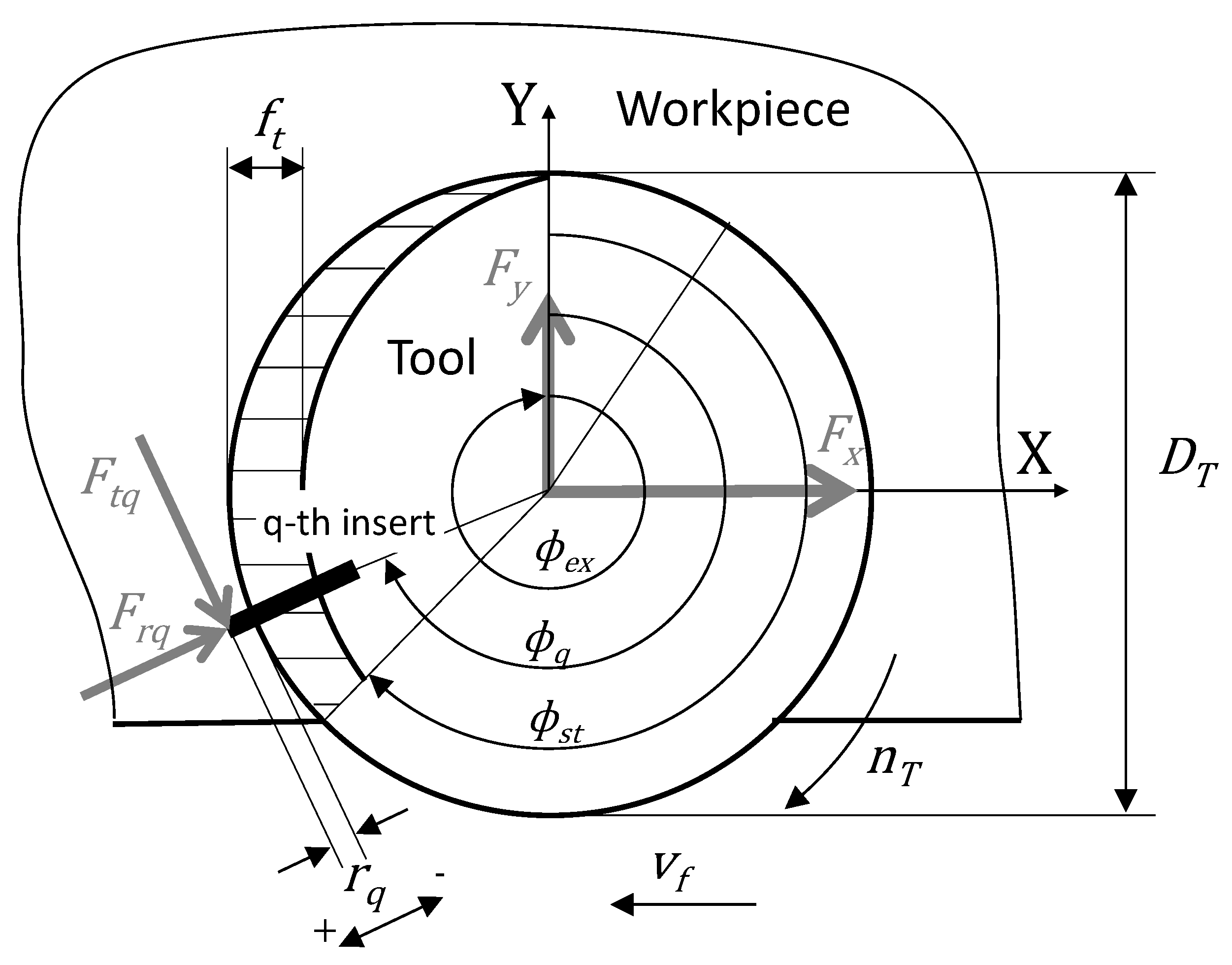
Figure 1.
Scheme of the face mill process.
Figure 1.
Scheme of the face mill process.
Figure 2.
Experimental set up for performing Pseudo-OMA.
Figure 2.
Experimental set up for performing Pseudo-OMA.
Figure 3.
Experimental setup for the milling tests.
Figure 3.
Experimental setup for the milling tests.
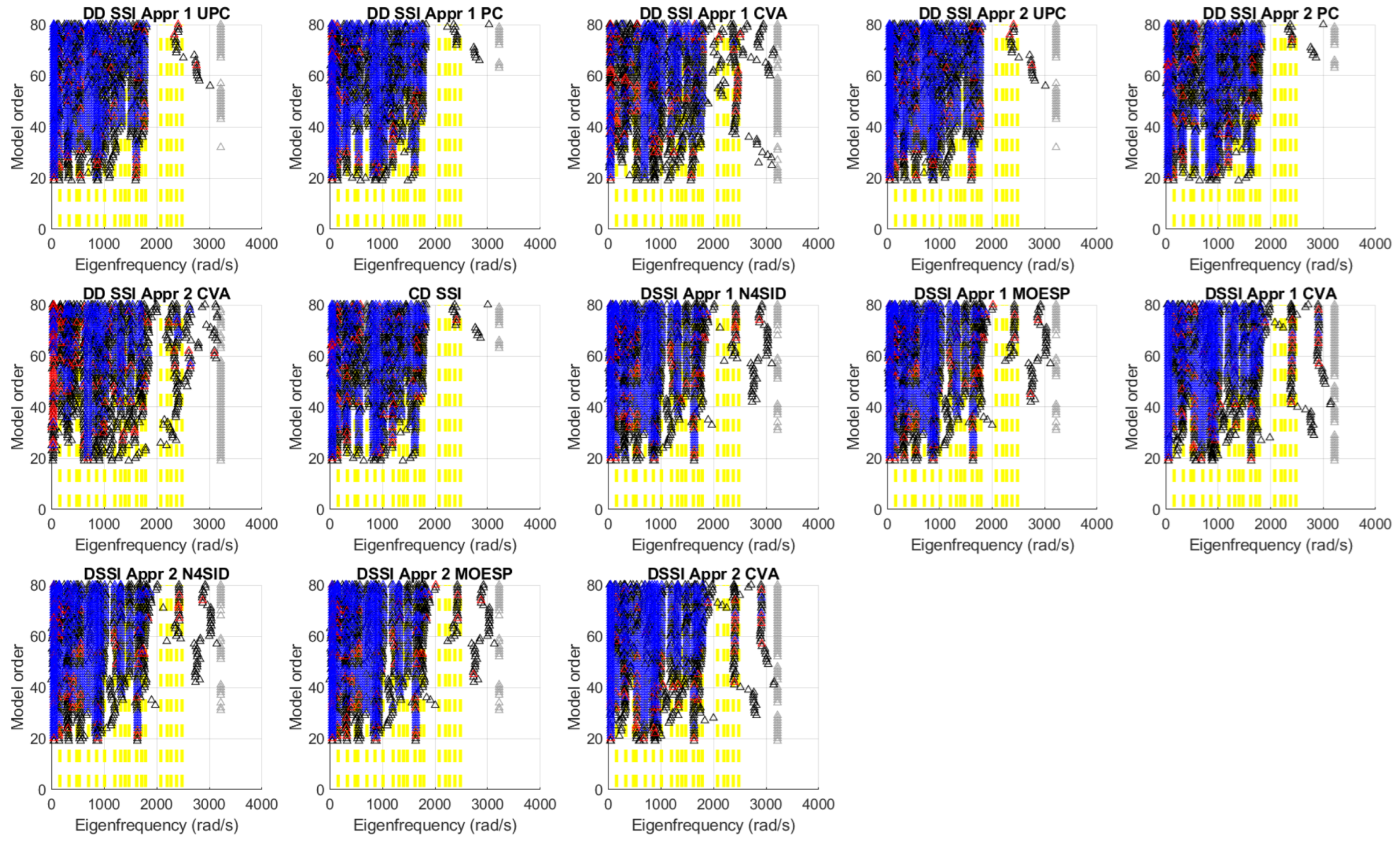
Figure 4.
Simulation No. 1—Correlated white noise excitation in all DOF—Stability diagram. Legend: gray colour—all eigenvalues, black colour—eigenvalues with physical meaning, red colour—eigenvalues being stable in the frequency, blue colour—eigenvalues being stable in the frequency and in the damping, yellow lines—reference eigenvalues.
Figure 5.
Simulation No. 1—Correlated white noise excitation in all DOF–MAC.
Figure 5.
Simulation No. 1—Correlated white noise excitation in all DOF–MAC.
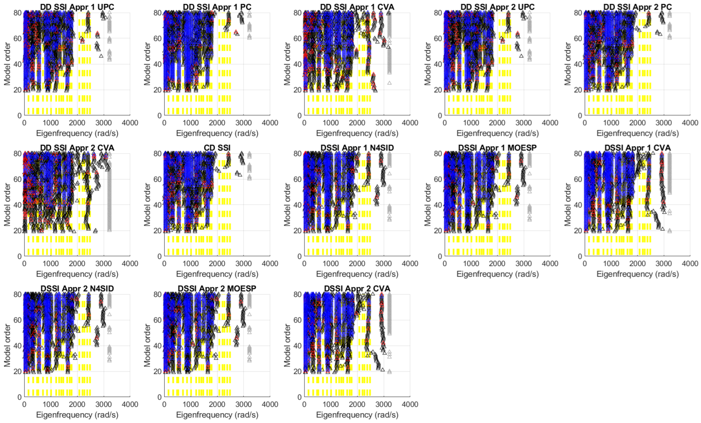
Figure 6.
Simulation No. 2—Correlated white noise excitation in all DOF and measurement noise of 1%—Stability diagram. Legend: gray colour—all eigenvalues, black colour—eigenvalues with physical meaning, red colour—eigenvalues being stable in the frequency, blue colour—eigenvalues being stable in the frequency and in the damping, yellow lines—reference eigenvalues.
Figure 7.
Simulation No. 3—Correlated white noise excitation in all DOF and measurement noise of 10%—Stability diagram. Legend: gray colour—all eigenvalues, black colour—eigenvalues with physical meaning, red colour—eigenvalues being stable in the frequency, blue colour—eigenvalues being stable in the frequency and in the damping, yellow lines—reference eigenvalues.
Figure 8.
Simulation No. 4—Uncorrelated white noise excitation in all DOF—Stability diagram. Legend: gray colour—all eigenvalues, black colour—eigenvalues with physical meaning, red colour—eigenvalues being stable in the frequency, blue colour—eigenvalues being stable in the frequency and in the damping, yellow lines—reference eigenvalues.
Figure 9.
Simulation No. 5—Uncorrelated white noise excitation in all DOF and measurement noise of 10%—Stability diagram. Legend: gray colour—all eigenvalues, black colour—eigenvalues with physical meaning, red colour—eigenvalues being stable in the frequency, blue colour—eigenvalues being stable in the frequency and in the damping, yellow lines—reference eigenvalues.
Figure 10.
Simulation No. 6—Uncorrelated white noise excitation in all DOF with different excitation levels—Stability diagram. Legend: gray colour—all eigenvalues, black colour—eigenvalues with physical meaning, red colour—eigenvalues being stable in the frequency, blue colour—eigenvalues being stable in the frequency and in the damping, yellow lines—reference eigenvalues.
Figure 11.
Simulation No. 7—White noise excitation in DOF 1—Stability diagram. Legend: gray colour—all eigenvalues, black colour—eigenvalues with physical meaning, red colour—eigenvalues being stable in the frequency, blue colour—eigenvalues being stable in the frequency and in the damping, yellow lines—reference eigenvalues.
Figure 12.
Simulation No. 8—White noise excitation in DOF 1 and measurement noise of 10%—Stability diagram. Legend: gray colour—all eigenvalues, black colour—eigenvalues with physical meaning, red colour—eigenvalues being stable in the frequency, blue colour—eigenvalues being stable in the frequency and in the damping, yellow lines—reference eigenvalues.
Figure 13.
Simulation No. 9—White noise excitation in DOF 2—Stability diagram. Legend: gray colour—all eigenvalues, black colour—eigenvalues with physical meaning, red colour—eigenvalues being stable in the frequency, blue colour—eigenvalues being stable in the frequency and in the damping, yellow lines—reference eigenvalues.
Figure 14.
Simulation No. 10—White noise excitation in DOF 2 and measurement noise of 10%—Stability diagram. Legend: gray colour—all eigenvalues, black colour—eigenvalues with physical meaning, red colour—eigenvalues being stable in the frequency, blue colour—eigenvalues being stable in the frequency and in the damping, yellow lines—reference eigenvalues.
Figure 15.
Simulation No. 11—White noise excitation in DOF 3—Stability diagram. Legend: gray colour—all eigenvalues, black colour—eigenvalues with physical meaning, red colour—eigenvalues being stable in the frequency, blue colour—eigenvalues being stable in the frequency and in the damping, yellow lines—reference eigenvalues.
Figure 16.
Simulation No. 12—White noise excitation in DOF 3 and measurement noise of 10%—Stability diagram. Legend: gray colour—all eigenvalues, black colour—eigenvalues with physical meaning, red colour—eigenvalues being stable in the frequency, blue colour—eigenvalues being stable in the frequency and in the damping, yellow lines—reference eigenvalues.
Figure 17.
Simulation No. 13—Process force excitation in DOF 3—Stability diagram. Legend: gray colour—all eigenvalues, black colour—eigenvalues with physical meaning, red colour—eigenvalues being stable in the frequency, blue colour—eigenvalues being stable in the frequency and in the damping, yellow lines—reference eigenvalues.
Figure 18.
Simulation No. 14—Broadband process force at point 3—Stability diagram. Legend: gray colour—all eigenvalues, black colour—eigenvalues with physical meaning, red colour—eigenvalues being stable in the frequency, blue colour—eigenvalues being stable in the frequency and in the damping, yellow lines—reference eigenvalues.
Figure 19.
Simulation No. 15—Broadband process force at point 3 and measurement noise 10%—Stability diagram. Legend: gray colour—all eigenvalues, black colour—eigenvalues with physical meaning, red colour—eigenvalues being stable in the frequency, blue colour—eigenvalues being stable in the frequency and in the damping, yellow lines—reference eigenvalues.
Figure 20.
Simulation No. 16—Broadband process force at point 3 and measurement noise 10%—Stability diagram for . Legend: gray colour—all eigenvalues, black colour—eigenvalues with physical meaning, red colour—eigenvalues being stable in the frequency, blue colour—eigenvalues being stable in the frequency and in the damping, yellow lines—reference eigenvalues.
Figure 21.
Simulation No. 17—Broadband process force at point 3 and measurement noise 10%—Stability diagram for and sampling frequency of 400 Hz. Legend: gray colour—all eigenvalues, black colour—eigenvalues with physical meaning, red colour—eigenvalues being stable in the frequency, blue colour—eigenvalues being stable in the frequency and in the damping, yellow lines—reference eigenvalues.
Figure 22.
Simulation No. 18—Broadband process force at point 3 and measurement noise 10% and process noise—Stability diagram for . Legend: gray colour—all eigenvalues, black colour—eigenvalues with physical meaning, red colour—eigenvalues being stable in the frequency, blue colour—eigenvalues being stable in the frequency and in the damping, yellow lines—reference eigenvalues.
Figure 23.
Simulation No. 19—Uncorrelated white noise signal in the three coordinates at TCP and measurement noise 10%—Stability diagram. Legend: gray colour—all eigenvalues, black colour—eigenvalues with physical meaning, red colour—eigenvalues being stable in the frequency, blue colour—eigenvalues being stable in the frequency and in the damping, yellow lines—reference eigenvalues.
Figure 24.
Simulation No. 20—Broadband process forces at TCP explicitly considered by the input vector and measurement noise 10%—Stability diagram. Legend: gray colour—all eigenvalues, black colour—eigenvalues with physical meaning, red colour—eigenvalues being stable in the frequency, blue colour—eigenvalues being stable in the frequency and in the damping, yellow lines—reference eigenvalues.
Figure 25.
Simulation No. 21—Broadband process forces excitation at TCP implicitly considered by the input vector and measurement noise 10%—Stability diagram. Legend: gray colour—all eigenvalues, black colour—eigenvalues with physical meaning, red colour—eigenvalues being stable in the frequency, blue colour—eigenvalues being stable in the frequency and in the damping, yellow lines—reference eigenvalues.
Figure 26.
Simulation No. 22—Broadband process forces excitation at TCP implicitly considered by the input vector, measurement noise 10%, and process noise as white noise signal—Stability diagram. Legend: gray colour—all eigenvalues, black colour—eigenvalues with physical meaning, red colour—eigenvalues being stable in the frequency, blue colour—eigenvalues being stable in the frequency and in the damping, yellow lines—reference eigenvalues.
Figure 27.
Simulation No. 23—Broadband process forces excitation at TCP implicitly considered by the input vector, measurement noise 10%, and process noise as a harmonic signal with a frequency of 672.3 Hz (depicted as red line)—Stability diagram. Legend: gray colour—all eigenvalues, black colour—eigenvalues with physical meaning, red colour—eigenvalues being stable in the frequency, blue colour—eigenvalues being stable in the frequency and in the damping, yellow lines—reference eigenvalues.
Figure 28.
Simulation No. 24—Broadband process forces excitation at TCP implicitly considered by the input vector, measurement noise 10%, and process noise as impulse sequence—Stability diagram. Legend: gray colour—all eigenvalues, black colour—eigenvalues with physical meaning, red colour—eigenvalues being stable in the frequency, blue colour—eigenvalues being stable in the frequency and in the damping, yellow lines—reference eigenvalues.
Figure 29.
Measured signals as process noise in various operational modes of the machine. Colours blue, green, red depict x, y, z directions, respectively.
Figure 29.
Measured signals as process noise in various operational modes of the machine. Colours blue, green, red depict x, y, z directions, respectively.
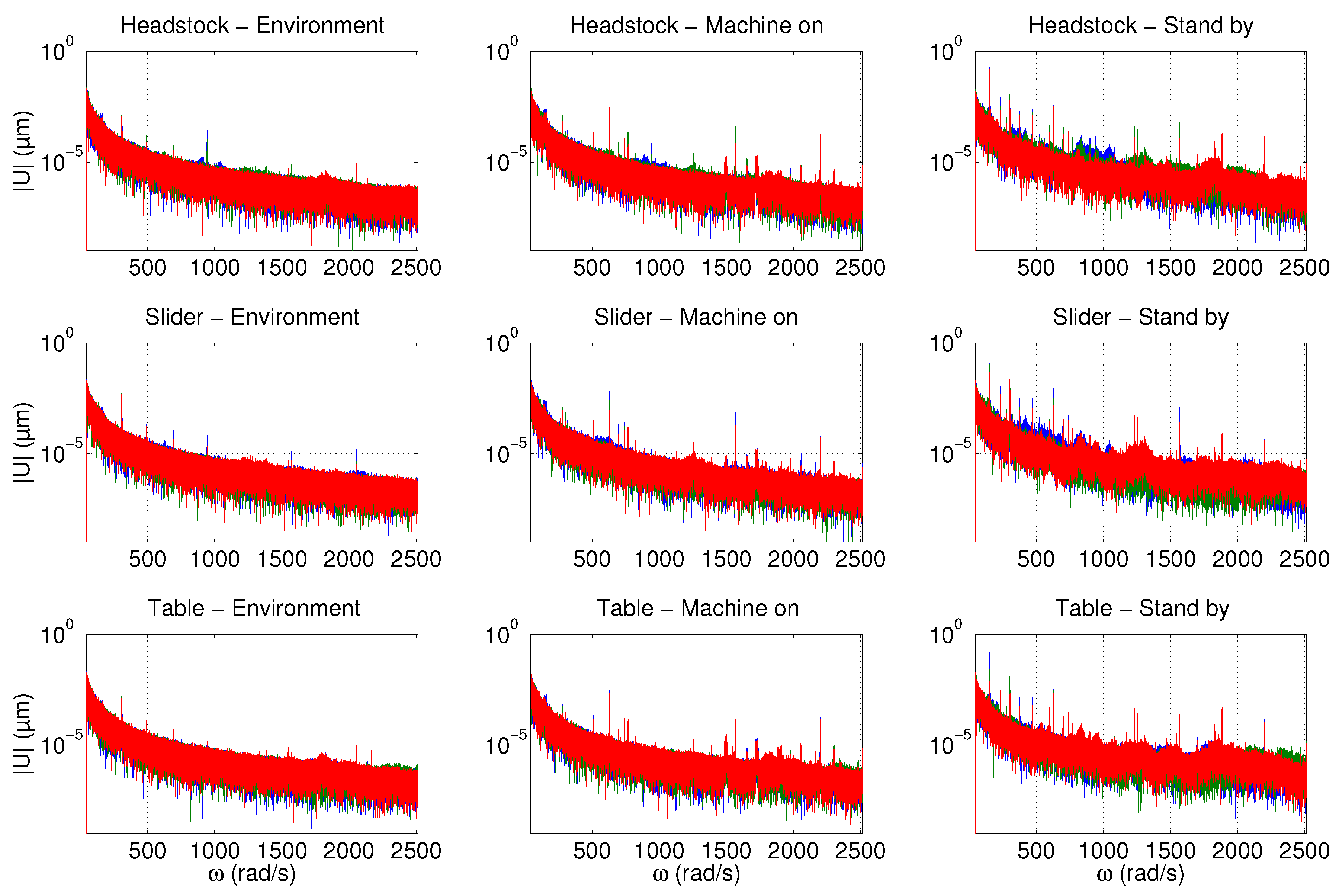
Figure 30.
Frequency spectrum of measured signals as process noise in various operational modes of the machine. Colours blue, green, red depict x, y, z directions, respectively.
Figure 30.
Frequency spectrum of measured signals as process noise in various operational modes of the machine. Colours blue, green, red depict x, y, z directions, respectively.
Figure 31.
Frequency spectrum of the real excitation force for Pseudo-OMA.
Figure 31.
Frequency spectrum of the real excitation force for Pseudo-OMA.
Figure 32.
Stability diagram for experiment No. 2—Shaker excitation with white noise and machine is off. Legend: gray colour—all eigenvalues, black colour—eigenvalues with physical meaning, red colour—eigenvalues being stable in the frequency, blue colour—eigenvalues being stable in the frequency and in the damping, yellow lines—reference eigenvalues.
Figure 33.
Stability diagram for the experiment No. 3—Shaker excitation with white noise and machine in the Stand by modus. Legend: gray colour—all eigenvalues, black colour—eigenvalues with physical meaning, red colour—eigenvalues being stable in the frequency, blue colour—eigenvalues being stable in the frequency and in the damping, yellow lines—reference eigenvalues.
Figure 34.
Stability diagram for experiment No. 4—Shaker excitation with white noise and impulse sequence as process noise. Legend: gray colour—all eigenvalues, black colour—eigenvalues with physical meaning, red colour—eigenvalues being stable in the frequency, blue colour—eigenvalues being stable in the frequency and in the damping, yellow lines—reference eigenvalues.
Figure 35.
Stability diagram for experiment No. 7—Shaker excitation with white noise and harmonic signal at the headstock as process noise. Legend: gray colour—all eigenvalues, black colour—eigenvalues with physical meaning, red colour—eigenvalues being stable in the frequency, blue colour—eigenvalues being stable in the frequency and in the damping, yellow lines—reference eigenvalues.
Figure 36.
Stability diagram for experiment No. 8—Shaker excitation with white noise and harmonic signal at the machine bed as process noise. Legend: gray colour—all eigenvalues, black colour—eigenvalues with physical meaning, red colour—eigenvalues being stable in the frequency, blue colour—eigenvalues being stable in the frequency and in the damping, yellow lines—reference eigenvalues.
Figure 37.
Stability diagram for experiment No. 9—Shaker excitation with white noise and harmonic signal at the slide of the y-axis as process noise. Legend: gray colour—all eigenvalues, black colour—eigenvalues with physical meaning, red colour—eigenvalues being stable in the frequency, blue colour—eigenvalues being stable in the frequency and in the damping, yellow lines—reference eigenvalues.
Figure 38.
Stability diagram for experiment No. 10—Shaker excitation with white noise and sinus swept signal at the headstock as process noise. Legend: gray colour—all eigenvalues, black colour—eigenvalues with physical meaning, red colour—eigenvalues being stable in the frequency, blue colour—eigenvalues being stable in the frequency and in the damping, yellow lines—reference eigenvalues.
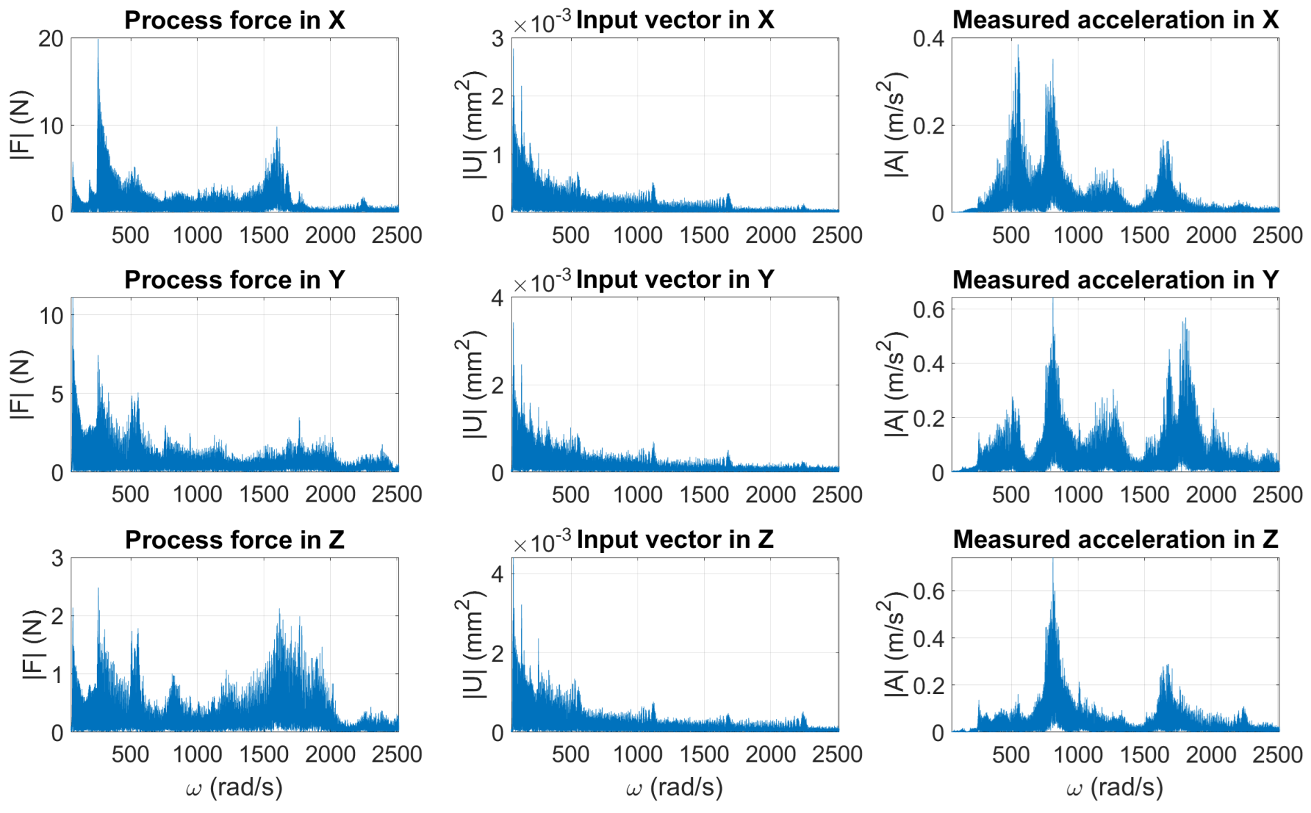
Figure 39.
Frequency spectra of the process forces, the input vectors and the measured acceleration at the headstock during the face milling.
Figure 39.
Frequency spectra of the process forces, the input vectors and the measured acceleration at the headstock during the face milling.
Figure 40.
Stability diagrams for the face milling experiment, response measured at the headstock and the input vector as the process force measured by RD. Legend: red colour—eigenvalues being stable in the frequency, blue colour—eigenvalues being stable in the frequency and in the damping, yellow lines—reference eigenvalues.
Figure 41.
Stability diagrams for the face milling experiment, response measured at the headstock and implicitly quantified input vector for a phase shift of 1.267 s. Legend: blue colour—eigenvalues being stable in the frequency and in the damping, yellow lines—reference eigenvalues.
Figure 41.
Stability diagrams for the face milling experiment, response measured at the headstock and implicitly quantified input vector for a phase shift of 1.267 s. Legend: blue colour—eigenvalues being stable in the frequency and in the damping, yellow lines—reference eigenvalues.
Figure 42.
Stability diagrams for the face milling experiment, response measured at the headstock and implicitly quantified input vector for a phase shift of 4.018 s. Legend: blue colour—eigenvalues being stable in the frequency and in the damping, yellow lines—reference eigenvalues.
Figure 42.
Stability diagrams for the face milling experiment, response measured at the headstock and implicitly quantified input vector for a phase shift of 4.018 s. Legend: blue colour—eigenvalues being stable in the frequency and in the damping, yellow lines—reference eigenvalues.
Figure 43.
Stability diagrams for the face milling experiment, response measured at the headstock and implicitly quantified input vector for a phase shift of 3.5 s. Legend: blue colour—eigenvalues being stable in the frequency and in the damping, yellow lines—reference eigenvalues.
Figure 43.
Stability diagrams for the face milling experiment, response measured at the headstock and implicitly quantified input vector for a phase shift of 3.5 s. Legend: blue colour—eigenvalues being stable in the frequency and in the damping, yellow lines—reference eigenvalues.
Table 1.
Investigated scenarios with the harmonic oscillator.
Table 1.
Investigated scenarios with the harmonic oscillator.
| Simulation | Description |
|---|
| No.1 | Correlated white noise in all DOF |
| No.2 | Correlated white noise in all DOF and measurement noise 1% |
| No.3 | Correlated white noise in all DOF and measurement noise 10% |
| No.4 | Uncorrelated white noise in all DOF |
| No.5 | Uncorrelated white noise in all DOF and measurement noise 10% |
| No.6 | Uncorrelated white noise in all DOF of various level (DOF 1—100%,
DOF 2—60%, DOF 3—30%) |
| No.7 | White noise at point 1 |
| No.8 | White noise at point 1 and measurement noise 10% |
| No.9 | White noise at point 2 |
| No.10 | White noise at point 2 and measurement noise 10% |
| No.11 | White noise at point 3 |
| No.12 | White noise at point 3 and measurement noise 10% |
| No.13 | Process forces at point 3 |
| No.14 | Broadband process forces at point 3 |
| No.15 | Broadband process forces at point 3 and measurement noise 10% |
| No.16 | Broadband process forces at point 3, measurement noise 10%, and |
| No.17 | Broadband process forces at point 3, measurement noise 10%, and Hz |
| No.18 | Broadband process forces at point 3, measurement noise 10%, and process noise |
Table 2.
Investigated scenarios with the machine model.
Table 2.
Investigated scenarios with the machine model.
| Simulation | Description |
|---|
| No.19 | Uncorrelated white noise excitation at TCP in all three coordinates |
| No.20 | Broadband process forces at TCP explicitly considered by the input vector |
| No.21 | Broadband process forces excitation at TCP implicitly considered by the input vector |
| No.22 | Broadband process forces excitation at TCP implicitly considered by the input vector, and process noise as white noise signal |
| No.23 | Broadband process forces excitation at TCP implicitly considered by the input vector, and process noise as harmonic signal |
| No.24 | Broadband process forces excitation at TCP implicitly considered by the input vector, and process noise as impulse sequence |
Table 3.
Investigated scenarios for Pseudo-OMA.
Table 3.
Investigated scenarios for Pseudo-OMA.
| Experiment | Description |
|---|
| No.1 | Process noise from the surroundings of the machine, i.e., machine is switched off |
| No.2 | Shaker excitation with white noise + machine off |
| No.3 | Shaker excitation with white noise + machine in stand by |
| No.4 | Shaker excitation with white noise + process noise due to pulse sequence at the headstock |
| No.5 | Shaker excitation with white noise + process noise due to pulse sequence at the machine table |
| No.6 | Shaker excitation with white noise + process noise due to pulse sequence at the machine slide |
| No.7 | Shaker excitation with white noise + process noise due to harmonic excitation with second shaker at the headstock |
| No.8 | Shaker excitation with white noise + process noise due to harmonic excitation with second shaker at the machine table |
| No.9 | Shaker excitation with white noise + process noise due to harmonic excitation with second shaker at the machine slide |
| No.10 | Shaker excitation with white noise + process noise due to sinus-swept excitation with second shaker at the headstock |
| No.11 | Shaker excitation with white noise + process noise due to sinus-swept excitation with second shaker at the machine table |
| No.12 | Shaker excitation with white noise + process noise due to sinus-swept excitation with second shaker at the machine slide |
Table 4.
MAC values for stochastic excitation of the oscillator (Mode shape pairs depicted as 1-1, 2-2, 3-3).
Table 4.
MAC values for stochastic excitation of the oscillator (Mode shape pairs depicted as 1-1, 2-2, 3-3).
| | | | No. 1 | No. 2 | No. 3 | No. 4 | No. 5 | No. 6 | No. 7 | No. 8 | No. 9 | No. 10 | No. 11 | No. 12 |
|---|
| DD SSI 1. approach | UPC | 1-1 | 1 | 1 | 1 | 1 | 1 | 1 | 1 | 1 | 1 | 1 | 1 | 1 |
| 2-2 | 1 | 1 | 1 | 1 | 1 | 1 | 1 | 1 | 1 | 1 | 1 | 1 |
| 3-3 | 0.96 | 0.98 | 0.75 | 1 | 1 | 1 | 1 | 1 | 1 | 1 | 1 | 1 |
| PC | 1-1 | NaN | 1 | 1 | 1 | 1 | 1 | NaN | 1 | NaN | 1 | NaN | 1 |
| 2-2 | NaN | 1 | 1 | 1 | 1 | 1 | NaN | 1 | NaN | 1 | NaN | 1 |
| 3-3 | NaN | 0.81 | NaN | 1 | 1 | 1 | 1 | 1 | NaN | 1 | 1 | 1 |
| CVA | 1-1 | NaN | 1 | 1 | 1 | 1 | 1 | NaN | 1 | NaN | 1 | NaN | 1 |
| 2-2 | NaN | 0.98 | 1 | 1 | 0.99 | 1 | NaN | 1 | 1 | 1 | NaN | 1 |
| 3-3 | NaN | 0.32 | NaN | 1 | 1 | 1 | NaN | 1 | 0.99 | 1 | 0.99 | 0.99 |
| DD SSI 2. approach | UPC | 1-1 | 1 | 1 | 1 | 1 | 1 | 1 | 1 | 1 | 1 | 1 | 1 | 1 |
| 2-2 | 1 | 1 | 1 | 1 | 1 | 1 | 1 | 1 | 1 | 1 | 1 | 1 |
| 3-3 | 0.96 | 0.98 | 0.75 | 1 | 1 | 1 | 1 | 1 | 1 | 1 | 1 | 1 |
| PC | 1-1 | NaN | 1 | 1 | 1 | 1 | 1 | NaN | 1 | 1 | 1 | NaN | 1 |
| 2-2 | NaN | 1 | 1 | 1 | 1 | 1 | NaN | 1 | 1 | 1 | NaN | 1 |
| 3-3 | NaN | 0.96 | NaN | 1 | 1 | 1 | NaN | 0.99 | NaN | 1 | NaN | 1 |
| CVA | 1-1 | NaN | 0.99 | 1 | 0.98 | 1 | 0.73 | NaN | 1 | NaN | 1 | NaN | 0.99 |
| 2-2 | NaN | 0.81 | 0.98 | 0.81 | 1 | 0.83 | NaN | 0.99 | NaN | 0.96 | NaN | 0.97 |
| 3-3 | NaN | 0.99 | 0.82 | 0.74 | 0.99 | 0.67 | NaN | 0.99 | NaN | 0.99 | NaN | 0.99 |
| CD SSI | - | 1-1 | 1 | 1 | 1 | 1 | 1 | 1 | 1 | 1 | 1 | 1 | 1 | 1 |
| 2-2 | 1 | 1 | 1 | 1 | 1 | 1 | 1 | 1 | 1 | 1 | 1 | 1 |
| 3-3 | 0.92 | 0.96 | NaN | 1 | 1 | 1 | 1 | 0.99 | 1 | 1 | 1 | 1 |
| DSSI 1. approach | N4SID | 1-1 | 1 | 1 | 1 | 1 | 1 | 1 | 1 | 1 | 1 | 1 | 1 | 1 |
| 2-2 | 1 | 1 | 1 | 1 | 1 | 1 | 1 | 1 | 1 | 1 | 1 | 1 |
| 3-3 | 1 | 0.96 | 0.72 | 1 | 1 | 1 | 1 | 1 | 1 | 1 | 1 | 1 |
| MOESP | 1-1 | 1 | 1 | 1 | 1 | 1 | 1 | 1 | 1 | 1 | 1 | 1 | 1 |
| 2-2 | 1 | 1 | 1 | 1 | 1 | 1 | 1 | 1 | 1 | 1 | 1 | 1 |
| 3-3 | 1 | 0.96 | 0.72 | 1 | 1 | 1 | 1 | 1 | 1 | 1 | 1 | 1 |
| CVA | 1-1 | 1 | 1 | 1 | 1 | 1 | 1 | 1 | 1 | 1 | 1 | 1 | 1 |
| 2-2 | 1 | 1 | 1 | 1 | 1 | 1 | 1 | 1 | 1 | 1 | 1 | 1 |
| 3-3 | 1 | 0.99 | 0.74 | 1 | 1 | 1 | 1 | 1 | 1 | 1 | 1 | 1 |
| DSSI 2. approach | N4SID | 1-1 | 1 | 1 | 1 | 1 | 1 | 1 | 1 | 1 | 1 | 1 | 1 | 1 |
| 2-2 | 1 | 1 | 1 | 1 | 1 | 1 | 1 | 1 | 1 | 1 | 1 | 1 |
| 3-3 | 1 | 0.94 | 0.78 | 1 | 1 | 1 | 1 | 1 | 1 | 1 | 1 | 1 |
| MOESP | 1-1 | 1 | 1 | 1 | 1 | 1 | 1 | 1 | 1 | 1 | 1 | 1 | 1 |
| 2-2 | 1 | 1 | 1 | 1 | 1 | 1 | 1 | 1 | 1 | 1 | 1 | 1 |
| 3-3 | 1 | 0.94 | 0.87 | 1 | 1 | 1 | 1 | 1 | 1 | 1 | 1 | 1 |
| CVA | 1-1 | 1 | 1 | 1 | 1 | 1 | 1 | 1 | 1 | 1 | 1 | 1 | 1 |
| 2-2 | 1 | 1 | 1 | 1 | 1 | 1 | 1 | 1 | 1 | 1 | 1 | 1 |
| 3-3 | 1 | 0.99 | 0.86 | 1 | 1 | 1 | 1 | 1 | 1 | 1 | 1 | 1 |
Table 5.
MAC values for excitation of the oscillator by process force.
Table 5.
MAC values for excitation of the oscillator by process force.
| | | | No. 13 | No. 14 | No. 15 | No. 16 | No. 17 | No. 18 |
|---|
| DD SSI 1. Algorithm | UPC | 1-1 | 1 | 1 | 1 | 1 | 1 | 1 |
| 2-2 | 0.99 | 1 | 1 | 1 | 1 | 1 |
| 3-3 | 1 | 0.99 | 1 | 1 | 0.99 | 1 |
| PC | 1-1 | NaN | NaN | 1 | 1 | 1 | 1 |
| 2-2 | NaN | NaN | 1 | 1 | 1 | 1 |
| 3-3 | 0.97 | NaN | 0.99 | 1 | 1 | 0.99 |
| CVA | 1-1 | NaN | NaN | 1 | 1 | 1 | 1 |
| 2-2 | NaN | NaN | 1 | 0.99 | 1 | 0.99 |
| 3-3 | 0.97 | NaN | 0.92 | 1 | 1 | 0.99 |
| DD SSI 2. Algorithm | UPC | 1-1 | 1 | 1 | 1 | 1 | 1 | 1 |
| 2-2 | 0.98 | 1 | 1 | 1 | 1 | 1 |
| 3-3 | 1 | 0.99 | 1 | 1 | 0.99 | 1 |
| PC | 1-1 | NaN | NaN | 1 | 1 | 1 | 1 |
| 2-2 | NaN | NaN | 1 | 1 | 1 | 1 |
| 3-3 | NaN | NaN | 1 | 1 | 0.99 | 1 |
| CVA | 1-1 | 1 | NaN | 1 | 0.99 | 1 | 1 |
| 2-2 | NaN | NaN | 0.96 | 0.95 | 0.92 | 0.96 |
| 3-3 | 0.97 | NaN | 0.96 | 0.86 | 0.99 | 0.96 |
| CD SSI | - | 1-1 | 1 | 1 | 1 | 1 | 1 | 1 |
| 2-2 | NaN | 1 | 1 | 1 | 1 | 1 |
| 3-3 | 0.97 | 1 | 1 | 1 | 0.99 | 1 |
| DSSI 1. Algorithm | N4SID | 1-1 | 1 | 1 | 1 | 1 | 1 | 1 |
| 2-2 | 0.97 | 1 | 1 | 1 | 1 | 1 |
| 3-3 | NaN | 1 | 1 | 1 | 1 | 1 |
| MOES. | 1-1 | 1 | 1 | 1 | 1 | NaN | 1 |
| 2-2 | 0.98 | 1 | 1 | 1 | 1 | 1 |
| 3-3 | 1 | 1 | 1 | 1 | 1 | 1 |
| CVA | 1-1 | 1 | 1 | NaN | 1 | 1 | 1 |
| 2-2 | 0 | 1 | 1 | 1 | 1 | 1 |
| 3-3 | 0 | 1 | 1 | 1 | 1 | 1 |
| DSSI 2. Algorithm | N4SID | 1-1 | 1 | NaN | NaN | NaN | 1 | 1 |
| 2-2 | 0.98 | 1 | 1 | 1 | 1 | 1 |
| 3-3 | NaN | 1 | 1 | 1 | 0.99 | 1 |
| MOES. | 1-1 | 1 | NaN | NaN | NaN | NaN | 1 |
| 2-2 | NaN | 1 | 1 | 1 | 1 | 1 |
| 3-3 | NaN | 1 | 1 | 1 | 0.9 | 1 |
| CVA | 1-1 | 1 | NaN | 1 | NaN | 1 | 1 |
| 2-2 | NaN | 1 | 1 | 1 | 1 | 1 |
| 3-3 | NaN | 1 | 1 | 1 | 0.99 | 1 |


