Figure 1.
Framework of the current work.
Figure 1.
Framework of the current work.
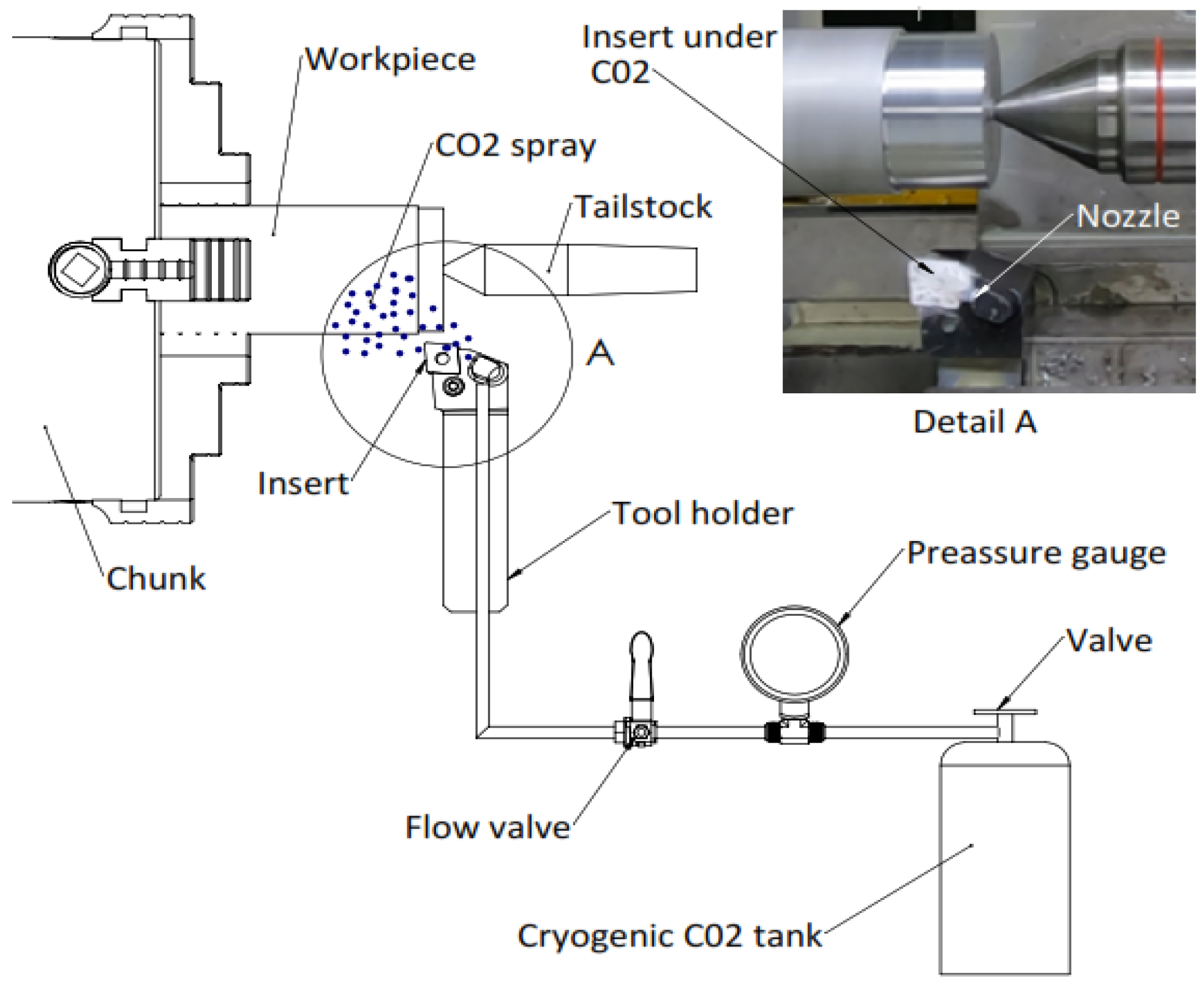
Figure 2.
Schematic diagram of cryogenic cutting system.
Figure 2.
Schematic diagram of cryogenic cutting system.
Figure 3.
Distribution of tests on cylindrical specimen.
Figure 3.
Distribution of tests on cylindrical specimen.
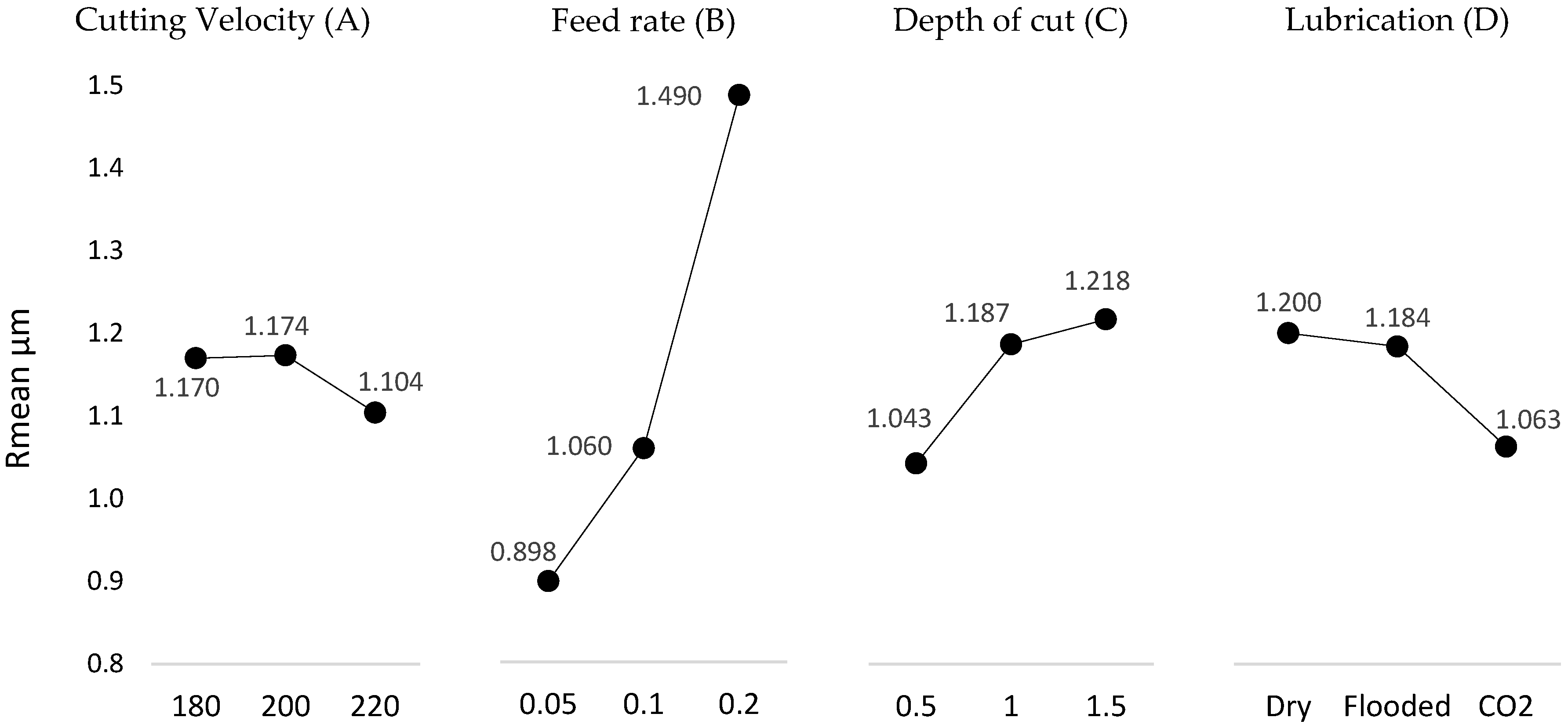
Figure 4.
Main effect plots for surface roughness response.
Figure 4.
Main effect plots for surface roughness response.
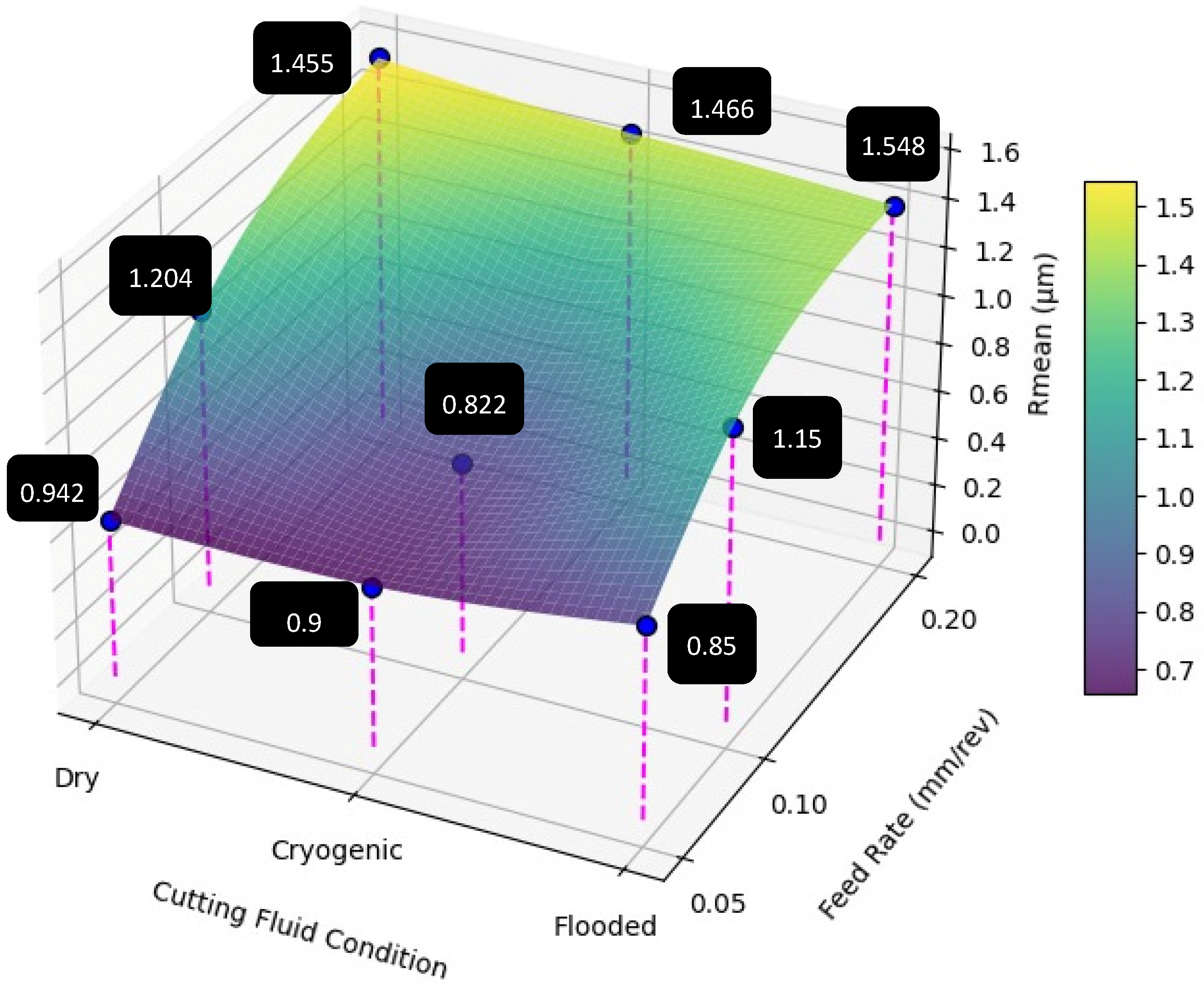
Figure 5.
Surface roughness vs. cutting fluid condition vs. feed rate.
Figure 5.
Surface roughness vs. cutting fluid condition vs. feed rate.
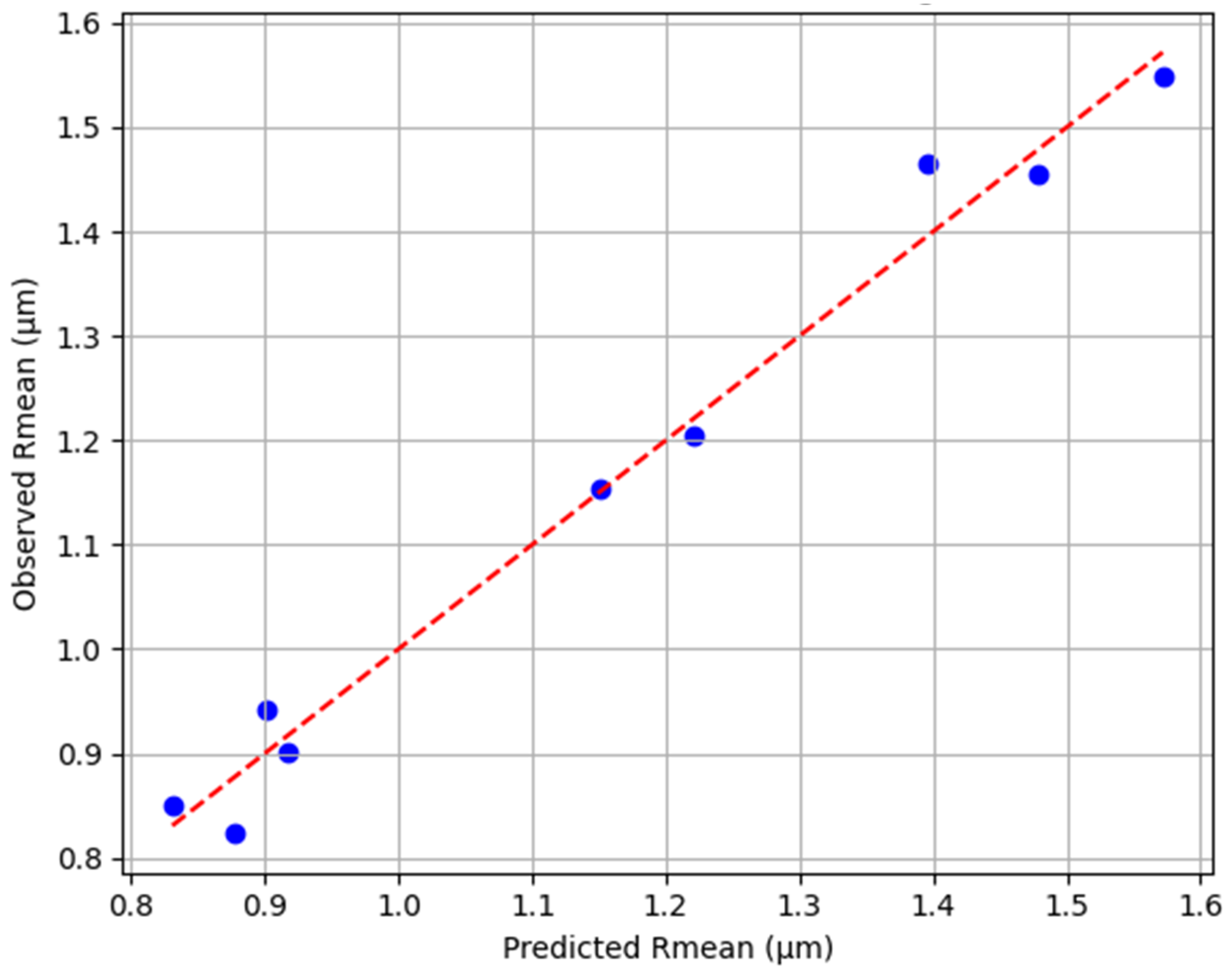
Figure 6.
Predicted (red dotted line) vs. observed surface roughness (blue dots).
Figure 6.
Predicted (red dotted line) vs. observed surface roughness (blue dots).
Figure 7.
Residual plot. The green dots represent the residuals (difference between the observed and the predicted values of the surface roughness). The red dotted line represents the zero line (no difference between predicted and observed values).
Figure 7.
Residual plot. The green dots represent the residuals (difference between the observed and the predicted values of the surface roughness). The red dotted line represents the zero line (no difference between predicted and observed values).
Figure 8.
SEM and EDX images of the machined surface for trial L1: (Cutting velocity: 180 m/min, feed rate: 0.2 mm/rev, depth of cut: 0.5 mm, cutting fluid condition: dry, and Ra mean value 1.455 µm). 1—plowing marks (6—zoomed-in view of the plowing mark). 2—worn surface indication. 3—cavities. 4—microchip adhesion. 5—D1, distance between plowing marks.
Figure 9.
SEM images of the machined surface for trial L3 (Cutting velocity: 180 m/min, feed rate: 0.05 mm/rev, depth of cut: 1.5 mm, cutting fluid condition: cryogenic, and Ra mean value: 0.901 µm). 1—plowing marks. 2—microchip adhesion. 3—cavities. 4—D1, distance between plowing marks.
Figure 9.
SEM images of the machined surface for trial L3 (Cutting velocity: 180 m/min, feed rate: 0.05 mm/rev, depth of cut: 1.5 mm, cutting fluid condition: cryogenic, and Ra mean value: 0.901 µm). 1—plowing marks. 2—microchip adhesion. 3—cavities. 4—D1, distance between plowing marks.
Figure 10.
SEM images of the machined surface for trial L7 ( Cutting velocity: 220 m/min, feed rate: 0.2 mm/rev, depth of cut: 1.5 mm, cutting fluid condition: flooded, and Ra mean value: 1.548 µm). 1—plowing marks. 2—deep depression mark. 3—cavities. 4—microchip adhesion. 5—D1, distance between plowing marks.
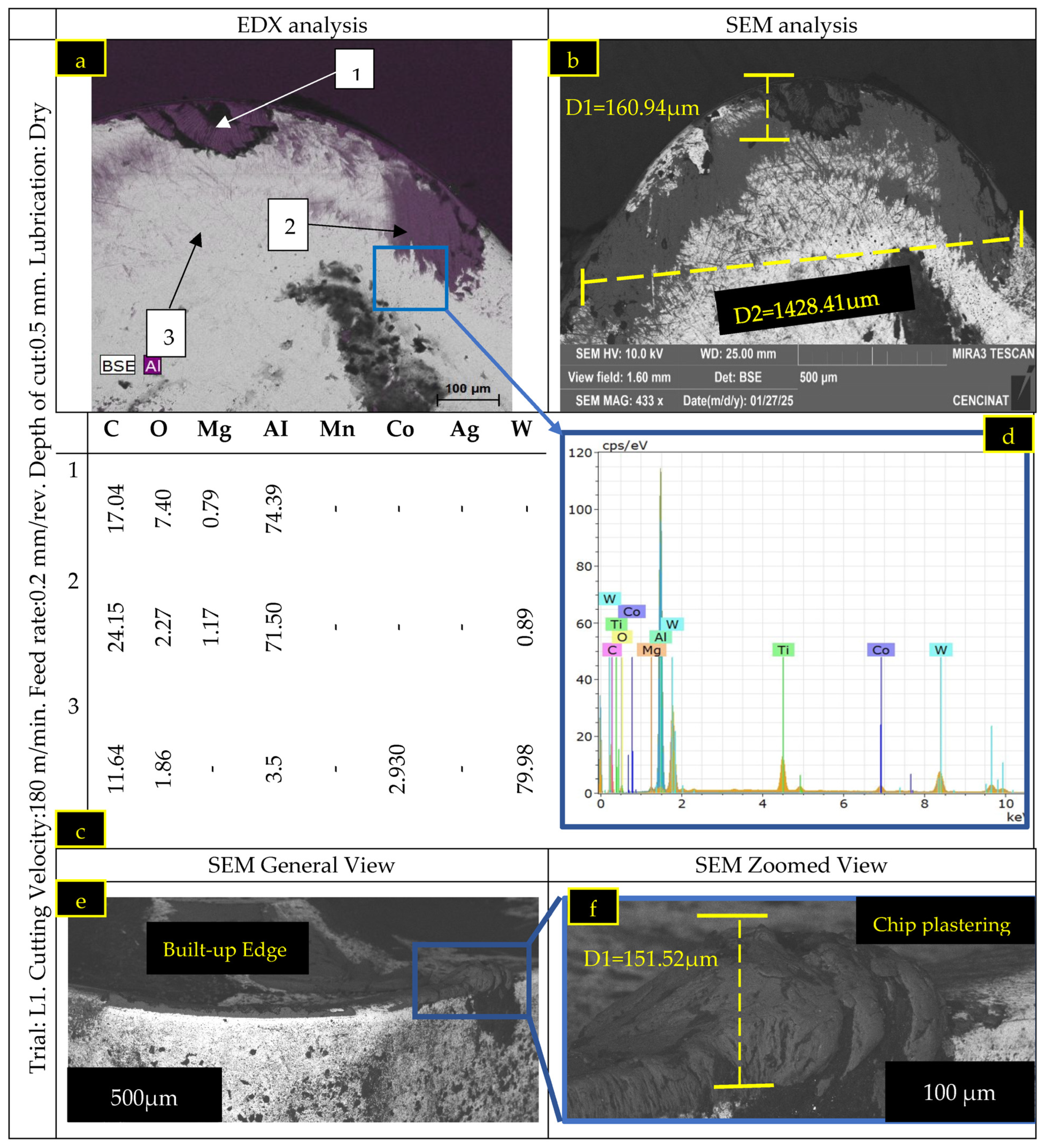
Figure 11.
SEM and EDX analysis of the tooltip. BUE formation after machining, trial L1. (a) EDX elemental map. 1, 2, and 3 are the points where elemental composition was carried out. (b) SEM micrograph. (c) Elemental composition of points 1–3. (d) Spectrum map. (e) BUE. (f) Zoomed-in view of BUE.
Figure 11.
SEM and EDX analysis of the tooltip. BUE formation after machining, trial L1. (a) EDX elemental map. 1, 2, and 3 are the points where elemental composition was carried out. (b) SEM micrograph. (c) Elemental composition of points 1–3. (d) Spectrum map. (e) BUE. (f) Zoomed-in view of BUE.
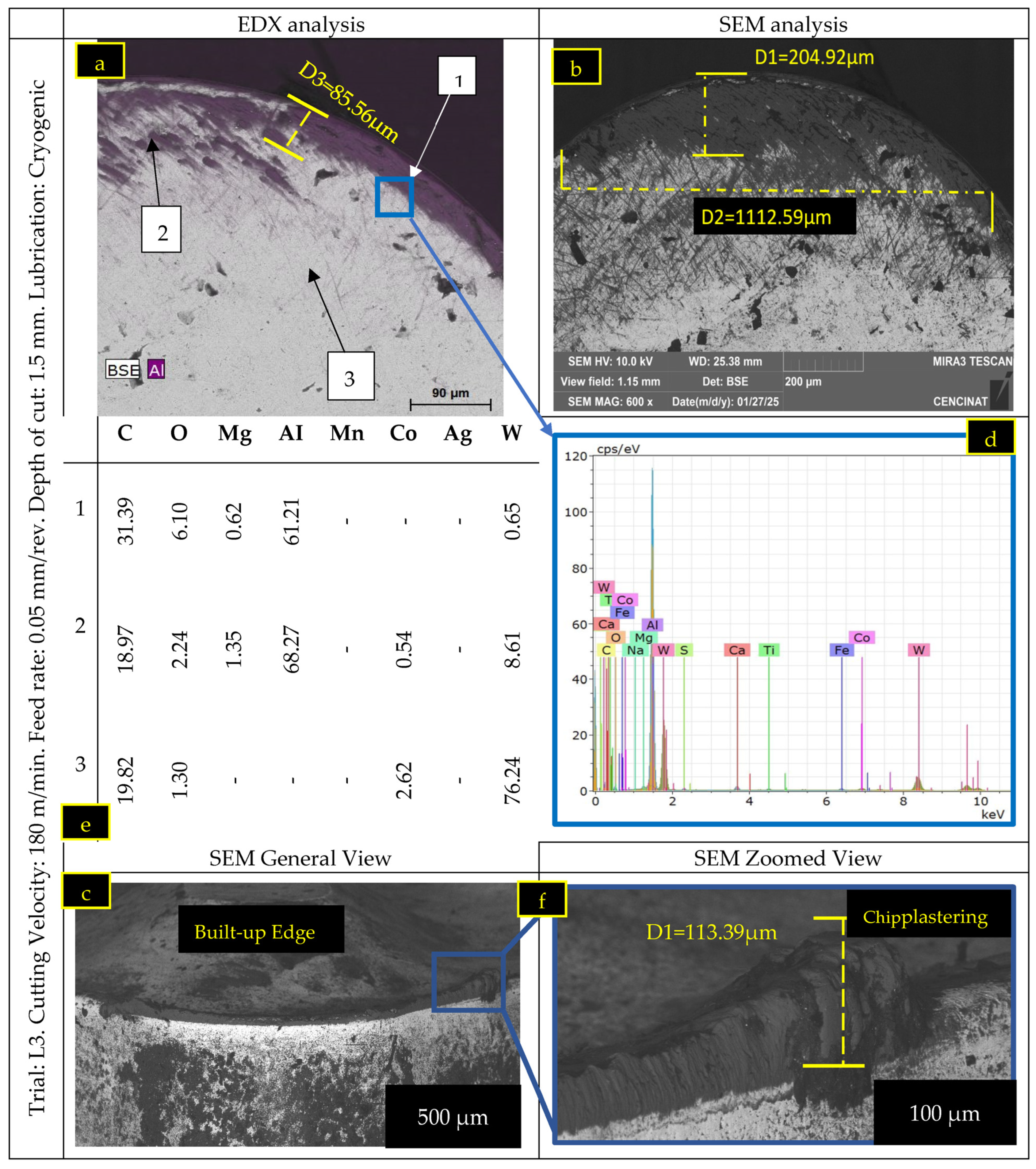
Figure 12.
SEM and EDX analysis of the tooltip. BUE formation after machining trial, L3. (a) EDX elemental map. 1, 2, and 3 are the points where elemental composition was carried out. (b) SEM micrograph. (e) Elemental composition of points 1–3. (d) Spectrum map. (c) BUE. (f) Zoomed-in view of BUE.
Figure 12.
SEM and EDX analysis of the tooltip. BUE formation after machining trial, L3. (a) EDX elemental map. 1, 2, and 3 are the points where elemental composition was carried out. (b) SEM micrograph. (e) Elemental composition of points 1–3. (d) Spectrum map. (c) BUE. (f) Zoomed-in view of BUE.
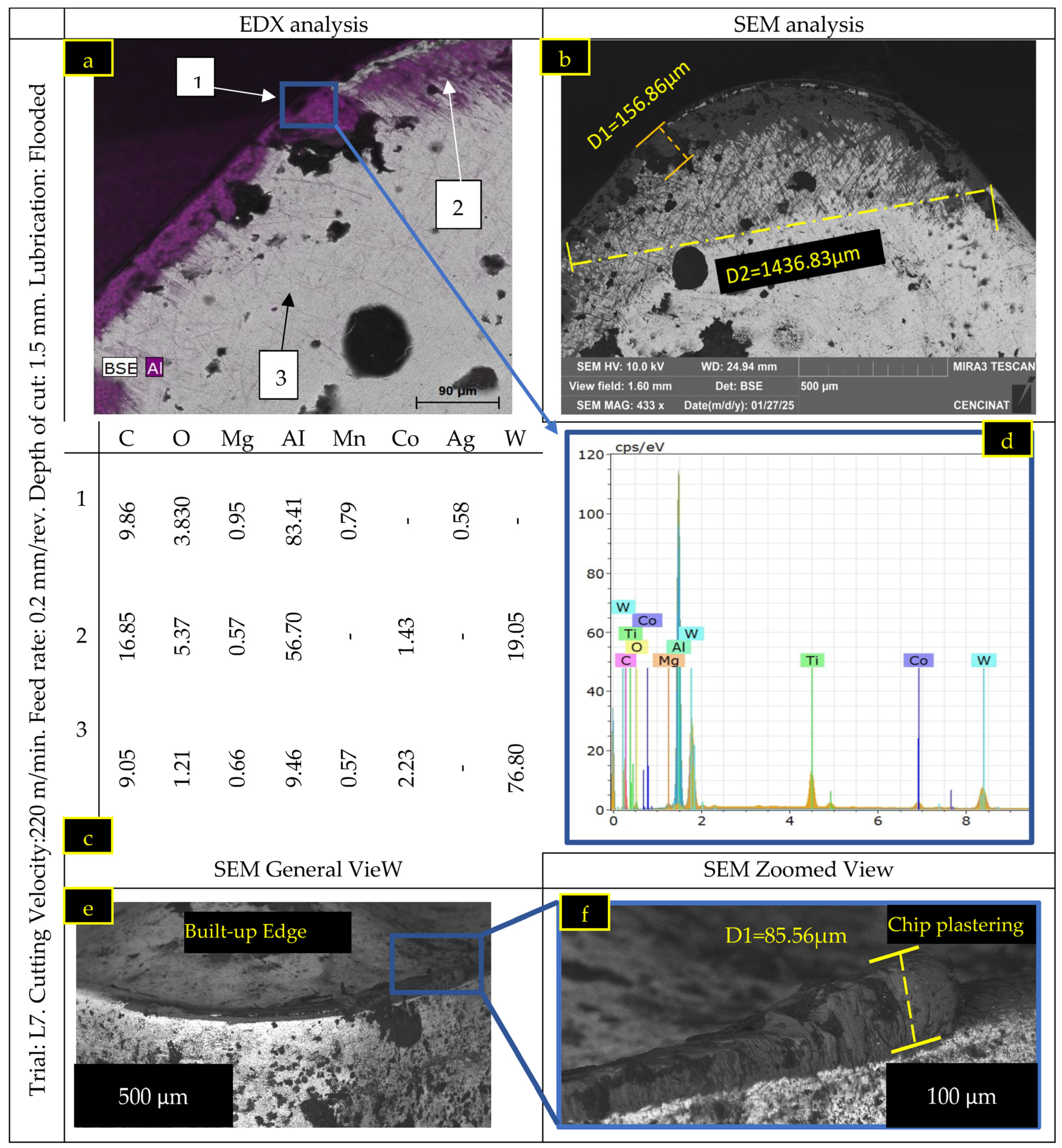
Figure 13.
SEM and EDX analysis of the tooltip. BUE formation after machining, trial L7. (a) EDX elemental map. 1, 2, and 3 are the points where elemental composition was carried out. (b) SEM micrograph. (c) Elemental composition of points 1–3. (d) Spectrum map. (e) BUE. (f) Zoomed-in view of BUE.
Figure 13.
SEM and EDX analysis of the tooltip. BUE formation after machining, trial L7. (a) EDX elemental map. 1, 2, and 3 are the points where elemental composition was carried out. (b) SEM micrograph. (c) Elemental composition of points 1–3. (d) Spectrum map. (e) BUE. (f) Zoomed-in view of BUE.
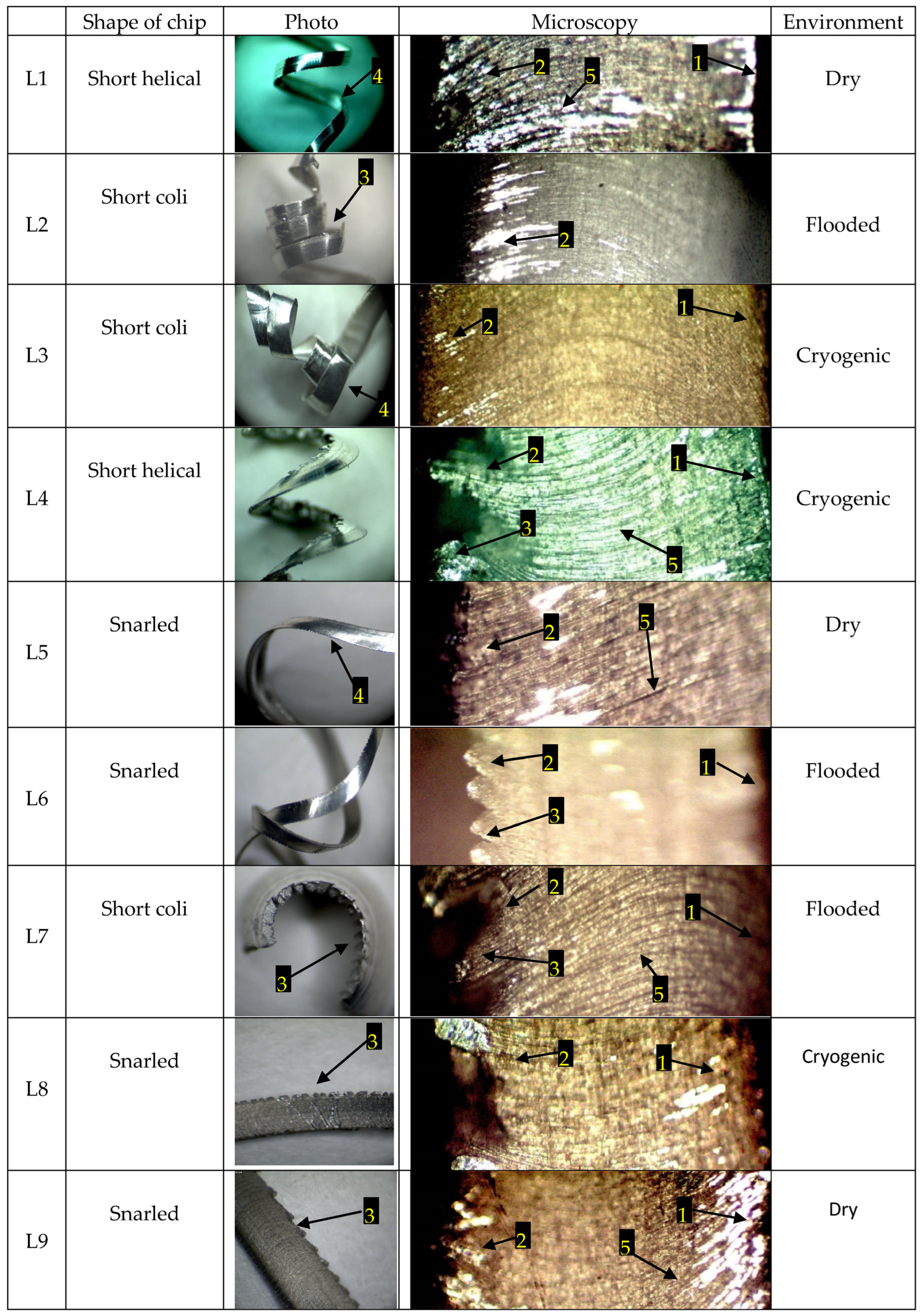
Figure 14.
Chip formation under dry, flooded, and cryogenic environments. Saw-tooth shapes in chip morphology: 1—primary serrated teeth, 2—secondary serrated teeth, 3—large serrations, 4—small serrations, 5—large scratches.
Figure 14.
Chip formation under dry, flooded, and cryogenic environments. Saw-tooth shapes in chip morphology: 1—primary serrated teeth, 2—secondary serrated teeth, 3—large serrations, 4—small serrations, 5—large scratches.
Table 1.
AI 7075-T6 material characterization.
Table 1.
AI 7075-T6 material characterization.
| Element (wt%) | Aluminum | Zinc | Copper | Iron |
|---|
| AI 7075-T6 | 89.71 | 6.13 | 1.78 | 0.18 |
Table 2.
Tool characteristics.
Table 2.
Tool characteristics.
| Tool insert | Specification | CNMG120408 P |
| Grade | K313 |
| Characteristics | Hard, low binder content, unalloyed WC/Co fine-grained |
| Manufacturer | Kennametal |
| Workpiece material | Non-ferrous materials/high-temp alloys |
| Chip braker | P |
| Tool holder | Specification | QS-PCLNR 2525 -12C |
| Characteristics | Nozzle for cooling |
Table 3.
Factors and levels selected for the experiment.
Table 3.
Factors and levels selected for the experiment.
| | Factors | Levels |
|---|
| 1 | 2 | 3 |
|---|
| A | Cutting speed (m/min) | 180 | 200 | 220 |
| B | Feed rate (mm/rev) | 0.05 | 0.1 | 0.2 |
| C | Depth of cut (mm) | 0.5 | 1 | 1.5 |
| D | Cutting fluid condition | Dry | Flooded | Cryogenic CO2 |
Table 4.
Orthogonal array L9 parameters.
Table 4.
Orthogonal array L9 parameters.
| Trials | A | B | C | D |
|---|
| L1 | 180 | 0.2 | 0.5 | Dry |
| L2 | 180 | 0.1 | 1 | Flooded |
| L3 | 180 | 0.05 | 1.5 | Cryogenic |
| L4 | 200 | 0.2 | 1 | Cryogenic |
| L5 | 200 | 0.1 | 1.5 | Dry |
| L6 | 200 | 0.05 | 0.5 | Flooded |
| L7 | 220 | 0.2 | 1.5 | Flooded |
| L8 | 220 | 0.1 | 0.5 | Cryogenic |
| L9 | 220 | 0.05 | 1 | Dry |
Table 5.
Profilometer configuration setting.
Table 5.
Profilometer configuration setting.
| Parameter | Value |
|---|
| Cut-off | 0.8 mm |
| Measure Length | 4.8 mm |
| Displacement Velocity | 1 mm/s |
| Magnification | 5000× |
Table 6.
Mean surface roughness using CNMG 120408 P.
Table 6.
Mean surface roughness using CNMG 120408 P.
| | Parameters | Surface Roughness µm |
|---|
| | A | B | C | D | R1 | R2 | R3 | Rmean | S/N |
|---|
| L1 | 180 | 0.2 | 0.5 | Dry | 1.459 | 1.45 | 1.457 | 1.455 | −3.259 |
| L2 | 180 | 0.1 | 1 | Flooded | 1.148 | 1.164 | 1.15 | 1.154 | −1.244 |
| L3 | 180 | 0.05 | 1.5 | Cryogenic | 0.903 | 0.901 | 0.898 | 0.901 | 0.909 |
| L4 | 200 | 0.2 | 1 | Cryogenic | 1.476 | 1.463 | 1.459 | 1.466 | −3.323 |
| L5 | 200 | 0.1 | 1.5 | Dry | 1.202 | 1.205 | 1.205 | 1.204 | −1.613 |
| L6 | 200 | 0.05 | 0.5 | Flooded | 0.851 | 0.852 | 0.85 | 0.851 | 1.401 |
| L7 | 220 | 0.2 | 1.5 | Flooded | 1.55 | 1.552 | 1.542 | 1.548 | −3.795 |
| L8 | 220 | 0.1 | 0.5 | Cryogenic | 0.822 | 0.826 | 0.82 | 0.823 | 1.696 |
| L9 | 220 | 0.05 | 1 | Dry | 0.944 | 0.942 | 0.94 | 0.942 | 0.519 |
Table 7.
ANOVA results of the raw data taken from CNMG 120408 P for surface roughness.
Table 7.
ANOVA results of the raw data taken from CNMG 120408 P for surface roughness.
| | Surface Roughness | |
|---|
| Factors | DF | S | V | F-Value | %P | p-Value | |
|---|
| Cutting Velocity (A) | 2 | 0.009 | 0.0046 | 22.907 | 1.396 | 0.042 | Significance |
| Feed rate (B) | 2 | 0.561 | 0.2806 | 1403.006 | 85.498 | 0.001 | Significance |
| Depth of cut (C) | 2 | 0.052 | 0.0261 | 130.538 | 7.955 | 0.008 | Significance |
| Lubrication (D) | 2 | 0.034 | 0.0169 | 84.537 | 5.152 | 0.012 | Significance |
| Error | 0 | | | | | | |
| Total | 8 | | | | 100 | | |
Table 8.
Response table for roughness means.
Table 8.
Response table for roughness means.
| | Surface Roughness |
|---|
| Level | A | B | C | D |
|---|
| 1 | 1.170 | 1.490 | 1.043 | 1.200 |
| 2 | 1.174 | 1.060 | 1.187 | 1.184 |
| 3 | 1.104 | 0.898 | 1.218 | 1.063 |
| Delta | 0.069 | 0.592 | 0.175 | 0.137 |
| Rank | 1 | 4 | 3 | 2 |
Table 9.
Response table for S/N means for CNMG 120408 P.
Table 9.
Response table for S/N means for CNMG 120408 P.
| | S/N Ratio |
|---|
| Level | A | B | C | D |
|---|
| 1 | −1.198 | −3.459 | −0.054 | −1.450 |
| 2 | −1.177 | −3.387 | −1.349 | −1.122 |
| 3 | −0.526 | 0.943 | −1.499 | −0.239 |
| Delta | 0.671 | 0.943 | 1.445 | 1.211 |
| Rank | 4 | 3 | 1 | 2 |
Table 10.
Confirmation test results for surface roughness.
Table 10.
Confirmation test results for surface roughness.
| | Initial Process Parameter | Optimal Process Parameters |
|---|
| | | Prediction S/N Ratio | Experiment |
|---|
| Level | A3, B2, C1, D3 | A3, B1, C1, D3 | A3, B1, C1, D3 |
|---|
| Surface roughness (µm) | 0.823 | | 0.736 |
| S/N ratio | 1.696 | 3.026 | 3.073 |
| Improvement in S/N ratio | 1.377 | | |
| Percentage reduction in surface 3.2roughness | %10.57 | | |
Table 11.
Regression coefficients and statistical metrics for Rmean model. Coefficient represents the estimated change in Ra (µm) for a one-unit change in the predictor, holding other variables constant. Std. Error indicates the uncertainty of each coefficient estimate; smaller values indicate more precise estimates. t is the test statistic (coefficient divided by its standard error). p-value quantifies the probability of observing such an effect if the true effect were zero; p < 0.05 is conventionally considered statistically significant.
| Term | Coefficient | Std. Error | t | p-Value |
|---|
| Intercept | 0.888000 | 0.263198 | 3.374 | 0.0433 |
| A | −0.001642 | 0.001264 | −1.298 | 0.2850 |
| B | 3.994286 | 0.331088 | 12.064 | 0.0012 |
| C | 0.174667 | 0.050575 | 3.454 | 0.0408 |
| Flooded | −0.016000 | 0.050575 | −0.316 | 0.7725 |
| Cryogenic | −0.137000 | 0.050575 | −2.709 | 0.0732 |

