Article

Bayesian Model Updating for Chatter in Milling

by
Ali Ebrahimi-Tirtashi
and
Keivan Ahmadi
*
Department of Mechanical Engineering, University of Victoria, Victoria, BC V8W 2Y2, Canada
*
Author to whom correspondence should be addressed.
J. Manuf. Mater. Process. 2025, 9(10), 323; https://doi.org/10.3390/jmmp9100323
Submission received: 5 August 2025 / Revised: 5 September 2025 / Accepted: 23 September 2025 / Published: 26 September 2025
(This article belongs to the Special Issue New Trends in Precision Machining Processes)

Abstract

The modal parameters of tooltip vibrations are crucial for determining chatter-free machining conditions. However, conventional methods often depend on measurements taken when the machine is not operating under real cutting conditions or require multiple experiments under chatter conditions, which is time-consuming and impractical for real-world manufacturing. This paper proposes a Bayesian Model Updating (BMU) approach to improve the chatter model parameters using experimental observations collected during normal, stable milling operations. Operational Modal Analysis (OMA) is adopted to extract the system dynamics from the in-process signals. These results are subsequently integrated into the BMU framework, updating the initial model parameters to reflect actual cutting conditions. The effectiveness of this approach is demonstrated through an experimental case study, highlighting its feasibility and potential for industrial applications.

1. Introduction

Regenerative chatter is a common and detrimental form of unstable self-excited vibration in machining. If not prevented, it can cause several adverse effects such as machine tool damage, poor surface finish, and accelerated tool wear, ultimately constraining the material removal rate and limiting overall machining productivity [1,2,3]. To suppress regenerative chatter in milling, stability analysis is employed to predict the boundary between stable and unstable cutting parameters. The results are typically presented in the form of a Stability Lobe Diagram (SLD), which determines regions of stability and instability as functions of spindle speed and axial depth of cut. These lobes are constructed by modeling the dynamic interaction between the machine tool structure and the cutting process, requiring the structural dynamics which are usually represented by the Frequency Response Function (FRF), or modal parameters measured at the tooltip or another highly flexible component of the setup [4,5].
The conventional approach to predicting modal parameters is through Experimental Modal Analysis (EMA), such as an impulse hammer test. However, a critical limitation arises because these tests are conducted while the machine is idle, with the spindle stationary and no cutting forces present. This idle state fails to capture the significant changes in system dynamics that occur under actual operational conditions. Consequently, an SLD based on an FRF from an idle-state EMA may be inaccurate in predicting chatter-free cutting parameters. To overcome this discrepancy and improve predictive accuracy, it is essential to calibrate or update the model parameters based on experimental observations collected while the machine is under operational conditions.
An effective approach to improving the chatter model’s accuracy is inverse chatter analysis, where the model parameters are tuned based on experimentally observed stability borders [6,7,8,9,10]. Machine Learning (ML) models have also been employed to construct SLD based on in-process sensor data [11,12,13,14,15]. By relying on operational measurements rather than offline modeling, both these approaches offer greater adaptability and accuracy in capturing the time-varying dynamics of machining processes. However, a key limitation is their reliance on extensive training datasets, which often require a significant amount of data collected under unstable cutting conditions, raising safety and productivity concerns in industrial applications. Alternatively, EMA can be performed using machining forces instead of an impulse hammer [16,17]. With this approach, the FRFs are measured during operation. However, since machining forces are harmonic at the spindle rotation frequency, specialized workpieces or experiments must be designed to broaden the excitation frequency spectrum. Computational models can also be used to predict FRF variations when dynamics are dominated by workpiece flexibility. For example, Rudel et al. [18] implemented a digital twin framework that couples FEM-based simulations with process modeling to predict chatter in a blade-integrated disk. Their work highlights the importance of adaptive modeling strategies for accurate chatter prediction in processes where structural dynamics evolve during machining.
Operational Modal Analysis (OMA) [19] has been adopted as a powerful technique for identifying system dynamics directly from vibration signals measured during the cutting process. Unlike modal testing, which characterizes the system’s structural dynamics, OMA captures the poles of the closed-loop machining system, reflecting the combined effects of the structural dynamics and the regenerative cutting process. Berthold et al. [20] explored OMA under operating conditions in milling, applying it alongside specially designed EMA tests to investigate differences in modal behavior. However, their study did not extract the full structural dynamics required to construct stability lobes for chatter prediction. Kim and Ahmadi [21] applied OMA to in-process vibration measurements during turning to extract the dominant system pole approaching instability. Building on this, a clustering-based algorithm was later introduced by Ebrahimi-Tirtashi and Ahmadi [22] to automate the OMA process for potential online applications. Zorlu et al. [23] further advanced the use of OMA by adapting it to milling operations, where the dynamics are Linear Time-Periodic (LTP), unlike the Linear Time-Invariant (LTI) dynamics in turning. To address this challenge, they adopted the lifting method, which enables mapping the LTP system into an equivalent LTI representation.
In this study, the OMA approach of Zorlu et al. [23] is coupled with Bayesian Model Updating (BMU) [24,25,26] to calibrate the modal parameters of the machining system based on the vibrations measured during standard, stable milling operations. Ahmadi introduced this approach for the LTI chatter dynamics in turning, which is often formulated accurately in the frequency domain [27]. However, its feasibility and practicality for the LTP chatter dynamics in milling are unexplored. Discrete-time domain methods such as the Semi-Discretization Method (SDM) [28,29] are widely used to link the structural modal parameters of the machine tool to the poles of the closed-loop time-periodic system, enabling the deterministic forward prediction of stability. BMU solves the inverse problem of adjusting the modal parameters (natural frequency, damping ratio, and stiffness) based on the closed-loop poles extracted by OMA from measured vibration signals. This results in a more accurate representation of the system’s in-process dynamics and improves the reliability of chatter stability predictions. We show that, unlike in turning, directly applying BMU in milling can be computationally prohibitive because it requires repeatedly estimating the eigenvalues of the state transition matrix in discrete-time domain models. To address this issue, we augment the BMU workflow with a surrogate function that approximates those eigenvalues accurately and efficiently enough to be used in the model updating algorithm.
In the following sections, we begin with a concise overview of milling chatter dynamics formulated in the discrete-time domain. We then describe how OMA is applied using the lifting method and TDPR framework developed by Zorlu et al. [23]. The poles identified in this process serve as inputs to the BMU framework presented in Section 2.2. To validate the effectiveness of the proposed method in predicting the stability boundary, both numerical simulations and an experimental case study are presented in Section 3.

2. Milling Dynamics

To model the dynamic interaction between the tool and workpiece during milling, a simplified representation of the structural system is first considered. A single-degree-of-freedom (SDOF) model is used here to simplify the explanation of the proposed approach. However, the method is general and can be extended to multi-degree-of-freedom (MDOF) systems to capture more complex structural dynamics.
Figure 1 illustrates an SDOF dynamic model representing the relative vibrations between the tool and the workpiece in milling. The structure is assumed to be flexible in the feed (X) direction, and the tool rotates about its axis at an angular speed of Ω . The regenerative effect introduces a delay τ = 2 π Ω N in the system response, resulting in the following Delay Differential Equation (DDE) [30]:
x ¨ ( t ) + 2 ζ x ω n x ˙ ( t ) + ω n 2 a H ( t ) ω n 2 k x x ( t ) = a H ( t ) ω n 2 k x x ( t τ )
where ζ x , ω n , and k x are the damping ratio, natural frequency, and stiffness, respectively. a is the nominal depth of cut, and H ( t ) is the cutting force directional coefficient, which is periodic with respect to the tooth-passing period τ , i.e., H ( t ) = H ( t + τ ) , and is defined as
H ( t ) = j = 1 N g j ( t ) K t cos θ j ( t ) K n sin θ j ( t ) sin θ j ( t ) g j ( t ) = 1 2 [ s g n ( θ j θ s t ) s g n ( θ j θ e x ) ]
where K t and K n are tangential and normal cutting coefficients, and g j ( t ) is a sign function that determines whether the tooth is in or out of cut. N is the number of teeth, and θ s t and θ e x are start and exit angles of a tooth to and from the cut, respectively.
One of the ways to determine the stability of vibrations governed by Equation (1) is using SDM, in which the delay interval τ is divided into equal subintervals of length Δ t   =   τ / r . Within each subinterval, the delayed state x ( t τ ) is assumed to be constant. This approximation transforms the original infinite-dimensional DDE into a finite-dimensional discrete-time system:
z i + 1 = D i z i z i = [ x i , x ˙ i , x i 1 , , x i r ] D i = exp ( A i Δ t ) 0 0 exp ( A i Δ t ) I A i 1 B i I 0 0 0 0 I 0 0 0 0 I 0
where z i is an augmented state vector that includes the state x ( t ) and its delayed values at each subinterval, and D i is the corresponding state transition matrix constructed from system matrices A i , B i as
A i = 0 1 ω n 2 ( 1 a H ( t ) / k x ) 2 ζ x ω n ;       B i = 0 a H ( t ) ω n 2 / k x
By recursively applying the transition matrices over one full delay period, the system’s monodromy matrix Φ is obtained:
Φ = D r 1 D r 2 D 0
The eigenvalues of matrix Φ correspond to the Floquet multipliers of the delayed periodic system described by Equation (1). Based on Floquet’s theorem for delayed LTP systems, the periodic motion loses stability when any eigenvalue of the monodromy matrix has a modulus greater than one.
Experimentally, the dominant multiplier of the milling dynamics can be obtained using the OMA approach presented by Zorlu et al. [23]. A summary of this approach is presented in the following subsection, and the resulting multipliers are used as observations in the proposed BMU framework to improve the chatter model.

2.1. Operational Modal Analysis

The lifting technique [31,32] is a method for transforming LTP systems into an equivalent LTI system by sampling the system’s response at fixed intervals synchronized with its periodicity. This results in a “lifted” system that evolves in discrete time, with each step representing one full period of the original system.
Considering the tool’s vibration along the x-axis, if r samples are taken during each tooth-passing period τ , the corresponding sampling time is given by Δ t = τ / r . Assuming that the observation window spans N c full tooth-passing intervals, the vibration measurements collected during the cth cycle ( c = 1 , , N c ) can be organized as follows:
M c = x c , 1 ,   x c , 2 ,   ,   x c , r
Here, x c , j refers to the jth sampled data point in the cth cycle, while x c , r denotes the final measurement in that cycle.
Although the measurement vector in Equation (6) is formed using data from one physical accelerometer, each row of this vector can be interpreted as the response of a virtual sensor that captures the tool tip motion at a consistent angular position within each tooth-passing cycle. Consequently, when this vector serves as the output of the lifted LTI model, the system’s periodic characteristics are effectively removed from the output. Thus, the lifted response matrix X can be organized as below, where each row shows the signal sampled once at period τ . For more details, refer to [23].
X = M 1     M N c = x 1 , 1 x 1 , 2 x 1 , r x N c , 1 x N c , 2 x N c , r
Various OMA methods can be employed to identify the dominant pole of the lifted time-independent dynamics, which also represents the dominant Floquet multiplier of milling dynamics. The Time Domain Polyreference (TDPR) method is an OMA technique used to identify the system poles of a vibratory system from its response under ambient or process-induced excitation [19]. In the context of machining, TDPR is particularly valuable for estimating the dominant poles of the closed-loop system dynamics during cutting operations without requiring external excitation sources [21,23].
TDPR constructs an autoregressive (AR) model of the system’s correlation functions (CF) derived from the measured response signals.
R X ( c ) = 1 N c c k = 1 N c c X k X k + c   ,   c = 0 , 1 , , N c 1
where X k denotes the kth column of the matrix X , representing the output of the kth lifted vibration signal. The companion matrix form of the AR model can be used to obtain the closed-loop pole of the system:
U d ( c + 1 ) = G U d ( c ) U d ( c ) = R X ( c n a + 1 ) R X ( c )
The eigenvalues of G represent the closed-loop poles of the system and quantify the stability of the process experimentally.
To distinguish physical poles from numerical artifacts introduced by overfitting, a stabilization diagram is constructed by incrementally increasing the model order. A pole is considered stabilized, and thus likely to represent a true system mode, if its frequency and damping ratio remain consistent across successive orders of the AR model. Given a discrete-time pole μ as an eigenvalue of G , the corresponding continuous-time pole is obtained as λ = ln ( μ ) Δ t . The corresponding estimated natural frequency ω ^ and the damping ratio ζ ^ are then computed as
ω ^ = | λ | ,   ζ ^ = Re ( λ ) | λ |
The dominant pole identified in this manner is used as a proxy for the system’s proximity to regenerative instability and can subsequently serve as the basis for the likelihood function in the BMU framework.

2.2. Model Updating

Let D represent the observations, i.e., dominant pole frequencies and damping ratios identified via OMA during the milling process. For a given model class M , the objective is to use these data to update the relative probability of each candidate model characterized by the parameter vector through the application of Bayes’ theorem [25,26]:
p ( θ | D , M ) = p ( D | θ , M ) p ( θ | M ) p ( D | M )
where p ( θ | D , M ) is the posterior PDF given the observation and model class M , p ( θ | M ) is the prior PDF which expresses the initial belief about the system and quantifies the prior plausibility of each model in the model class M , and p ( D M ) is the evidence or marginal likelihood for the model class M provided by data D and serves as the normalizing constant in Bayes’ theorem to ensure that the posterior distribution integrates to one. p ( D | θ , M ) is the likelihood function which quantifies the agreement between the experimental observations (i.e., the dominant closed-loop pole’s damping ratio and frequency identified by OMA) and their theoretical counterpart predicted by the SDM for a given set of parameter variations θ . Specifically, let ω ^ p , j and ζ ^ p , j denote the frequency and damping ratio of the dominant pole identified from the jth OMA repetition at the pth combination of cutting depth and spindle speed.
The likelihood is then given by
p ( D θ , M ) = j = 1 N s p = 1 N p p ( ω ^ p , j θ , M ) p ( ζ ^ p , j θ , M )
where N p is the number of tested cutting pairs, and N s is the number of OMA repetitions per pair. The connection between the measured dominant pole through OMA and the predicted one is given in terms of the prediction error as
ω ^ p , j = ω p + e ω p , j ,       ζ ^ p , j = ζ p + e ζ p , j
and the prediction errors are assumed to follow independent zero-mean Gaussian distributions with variances σ ω 2 and σ ζ 2 , respectively. Thus, the likelihood function can be written as
p ( D | θ , M ) = 1 2 π σ ω σ ζ exp ( 1 2 p = 1 N p J p ( θ ) ) , J p ( θ ) = j = 1 N s ( ω ^ p , j ω p ( θ ) ) 2 σ ω 2 + ( ζ ^ p , j ζ p ( θ ) ) 2 σ ζ 2
When Bayesian updating is applied with the parameter vector θ including the prediction error variances for frequency and damping ratio σ ω 2 and σ ζ 2 , it is important to select their prior distributions carefully. The chosen priors must ensure that the relative influence of frequency and damping components in the likelihood function is properly balanced, so that neither dominates the posterior update and both contribute meaningfully to the identification of modal parameters. To manage this balance, following the evidence-based approach proposed by Goller et. al. [26], multiple model classes M ( α k ) ,   k = 1 N k are defined, in which the ratio of prediction-error variances for damping and frequency is fixed at α k = σ ζ σ ω . The likelihood function for the model class M k , where M k is shorthand for M ( α k ) , is obtained by substituting α k into Equation (14) as
J p ( θ ) = j = 1 N s ( ω ^ p , j ω p ( θ ) ) 2 σ ω 2 + ( ζ ^ p , j ζ p ( θ ) ) 2 ( α k σ ω ) 2
Here, θ = [ θ ω ,   θ ζ ,   θ k ,   σ ω ] , where the random variables θ ω , θ ζ , and θ k represent the relative variations of the system’s true modal parameters from their respective nominal values, defined as
ω n = ω ¯ n ( 1 + θ ω ) ζ x = ζ ¯ x ( 1 + θ ζ ) k x = k ¯ x ( 1 + θ k )
Beyond updating the structural modal parameters within each individual model class M k , a second layer of Bayesian inference is employed to evaluate and compare multiple model classes corresponding to different values of the weighting parameter α . This approach allows us to determine which model class is more likely to describe the observed data. In doing so, it identifies the most appropriate value of α , which defines the optimal balance between the contributions of closed-loop frequency and damping ratio prediction errors in the likelihood function. The appropriate Bayes’ theorem at the model class level is [26]
p ( M k D , M ) = p ( D | M k ) p ( M k | M ) p ( D | M )
where M is a set of N k model classes M k .
Calculating the model evidence (marginal likelihood) analytically in Bayesian inference is often impractical, due to the high-dimensional integration required over the parameter space. To address this challenge, sampling-based methods are commonly employed to approximate the posterior distribution without explicitly computing the evidence [33,34]. Among these, Transitional Markov Chain Monte Carlo (TMCMC) [35] is particularly suitable for our application, as it not only facilitates efficient sampling through a sequence of intermediate distributions bridging the prior and posterior but also provides a natural and accurate estimate of the model evidence. This capability makes TMCMC especially advantageous when performing Bayesian model selection, where comparing the marginal likelihoods of candidate models p ( D | M k ) is essential for determining the most plausible explanation of observed data p ( D | θ , M ) [36].
To evaluate the likelihood function in this study, we need to predict the dominant closed-loop pole or, in other words, its frequency and damping ratio, for each candidate set of modal parameters. This is achieved by building the discrete-time monodromy matrix of the system ( G ) and calculating its eigenvalues. However, doing this many times during the TMCMC sampling becomes computationally prohibitive due to the size and complexity of the matrices involved. In this study, at each TMCMC sample, the eigenvalues of the 42 × 42 monodromy matrix corresponding to the delay period τ , which is divided into r = 40 intervals, must be computed multiple times for different model parameters ( θ ).
To establish credibility bounds in the stability lobe diagram, the uncertainty in the eigenvalues must be quantified using the posterior distribution of the parameters. Let μ m ( θ ) denote the dominant eigenvalue of the monodromy matrix as a function of the parameter vector θ . By expanding μ m ( θ ) using a second-order perturbation method [37], the mean eigenvalue can be approximated as
μ ¯ m = E [ μ m ( θ m ) ] = μ m ( 0 ) + 1 2 Trace ( Σ θ D μ ) ,
and its variance as
E ( μ m ( θ m ) μ ¯ m ) ( μ m ( θ m ) μ ¯ m ) * = d μ T Σ θ d μ * + 1 2 Trace ( Σ θ D μ Σ θ D μ * ) ,
where d μ and D μ are the gradient and Hessian of the eigenvalue with respect to θ m , and Σ θ is the posterior covariance matrix of the parameters. These expressions are used to construct upper and lower credibility bounds by offsetting the eigenvalue contour by one standard deviation.
To reduce the computational cost, a surrogate model is trained to estimate the relationship between the modal parameters and the dominant pole characteristics. In this study, we use a Gaussian Process Regression (GPR) model [38] with a Matérn kernel to predict the closed-loop frequency and damping ratio based on the modal parameters. The surrogate model is trained using a set of parameter samples selected from a uniform grid covering the range of the prior distribution. For each sample, the full-order model is run once to calculate the dominant eigenvalue of the system’s transition matrix. This eigenvalue is then converted into its corresponding continuous-time frequency and damping ratio, which are used as the target outputs for training the GPR model. Once the surrogate model is trained, it can quickly estimate the system’s dynamic response for any set of modal parameters. This makes it possible to evaluate the likelihood function much faster than computing eigenvalues directly, greatly reducing the overall cost of the TMCMC-based Bayesian updating process.

3. Results and Discussion

3.1. Numerical Simulation

To verify the effectiveness of the Bayesian Model Updating (BMU) approach in calibrating the modal parameters and quantifying the uncertainties in the milling process, a numerical simulation was performed on a single-degree-of-freedom (SDOF) system.
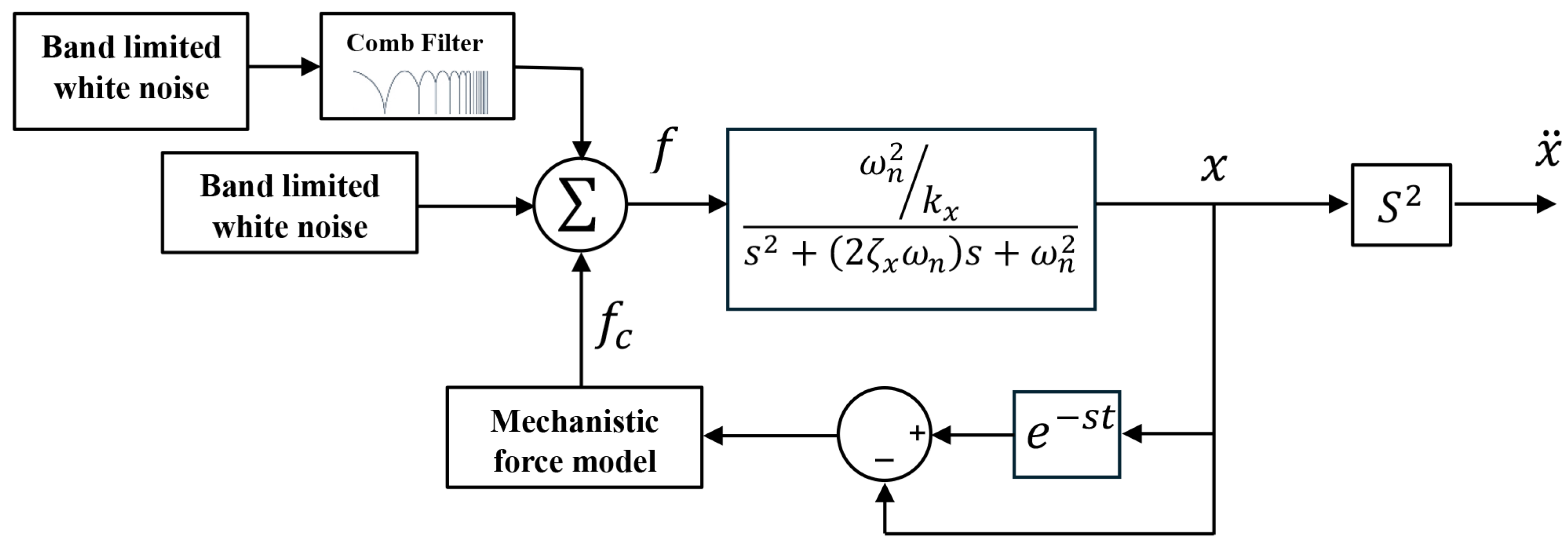
Figure 2 shows the block diagram used to simulate the single-degree-of-freedom (SDOF) milling dynamics numerically, considering K t = 650 MPa and K n = 110 MPa for tangential and normal cutting force coefficients, and the dynamics of tool–workpiece assembly are considered as ω n = 2 π × 194 rad/s, ζ x = 0.005 , and k x = 2.35 N/ μ m for the natural frequency, damping ratio, and stiffness, respectively.
The stability lobe diagrams of the setup, obtained by the SDM, are shown in Figure 3. The input force consists of periodic machining forces superimposed by broadband white noise to account for the random forces during the process. Simulations were conducted in MATLAB Simulink 2023b. Process vibrations were simulated for milling with 2000 and 2100 RPM spindle speeds and various stable DOC values marked with circles on the SLD in Figure 3.
The power spectral density (PSD) of the simulated acceleration at 2100 RPM and a 0.4 mm depth is displayed in Figure 4. The PSD of the simulated vibrations shows peaks at the tooth-passing frequency harmonics and a non-harmonic peak at around 195.8 Hz.
The measured signals are lifted at the tooth-passing period and organized in the measurement matrix, X , described in Equation (7). Subsequently, treating each row of the X matrix as a separate lifted sensor, we computed the PSD matrix of the lifted sensors; the top singular value of the resulting PSD is shown in Figure 5. The Nyquist frequency of the signals after lifting reduces to half of the tooth-passing frequency, f t p / 2 = 35 Hz.
Since milling dynamics are periodic, according to Floquet theory, the spectrum exhibits frequency components at f c ± k × f t p and f c ± k × f t p , where k is an integer, f c represents the oncoming chatter frequency, and f t p denotes the tooth-passing frequency [39]. Considering that the response before lifting shows a chatter frequency of 195.8 Hz, after lifting, this frequency is aliased to one of its harmonics at around 14.2 Hz, which corresponds to f c + 3 × f t p .
The stabilization diagram resulting from the TDPR identification of the lifted response at point P with various model orders n a is shown in Figure 5. While the diagram includes a mix of physical and spurious poles, the column of circles with similar shading indicates a physical pole at the corresponding frequency.
The dominant pole was identified at N p = 7 combinations of spindle speed and cutting depth, and identification was repeated N s = 10 times at each combination. The mean value and standard deviation of the identified poles are shown in Table 1.
To reduce the high computational cost associated with repeatedly evaluating the likelihood function in TMCMC, particularly the eigenvalue analysis of the state transition matrix G , a GPR surrogate model with a Matérn kernel was employed. This surrogate was trained to approximate the dominant closed-loop frequency and damping ratio as functions of the model parameters [ θ ω , θ ζ , θ k ] , which represent expected variations in the natural frequency, damping ratio, and mode shape scaling, respectively. These parameter ranges were uniformly sampled to reflect the prior distribution based on initial uncertainty. A training dataset consisting of 1000 combinations of model parameters was used to construct the GPR model. Once trained, the surrogate provides rapid predictions of the closed-loop poles for any arbitrary parameter combination required by the TMCMC algorithm, thereby enabling efficient and accurate sampling of the posterior distribution without recomputing expensive matrix operations at every iteration.
The prior distributions of the model parameters, θ , are assumed to be uniform over the range [ 0.3 , 0.3 ] , and the prior distribution of the prediction error variance, σ ω 2 , is taken as uniform over the interval [ 0 , 1 ] .
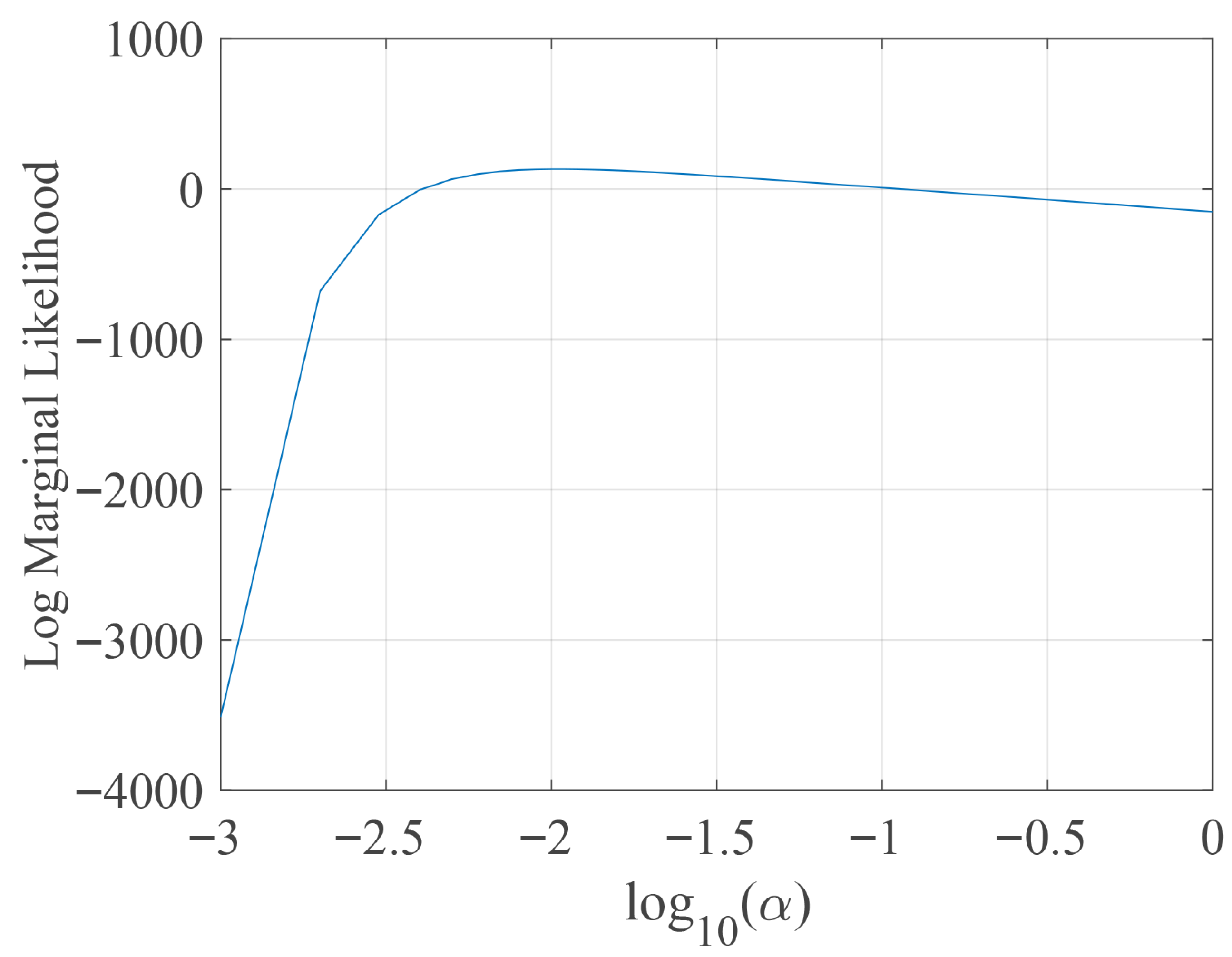
The TMCMC algorithm was employed to generate 5000 samples from the posterior distribution of the model parameters across model classes with α k over the range of 0.001 to 1. The model evidence (log marginal likelihood) for each class was also computed using TMCMC and is presented in Figure 6. The evidence reaches its maximum at α   =   0.01 , indicating that this model class has the highest plausibility among the candidates. Consequently, the model class corresponding to this amount is selected for parameter updating.
For the selected model class, samples were generated from the posterior distribution of the three model parameters. The diagonal plots in Figure 7 show the histograms of each parameter, while the off-diagonal plots display scatter views of the samples from the prior (gray points) and the posterior (green points).
Since the analysis is conducted entirely through numerical simulation, the dominant closed-loop poles computed mathematically from the discretized state-space model and those identified through OMA yield identical results. This equivalence is evident in the plotted figure, where all the estimated parameter variations converge to zero. The convergence indicates that the posterior distributions of the model parameters remain centered at their nominal values, confirming that the closed-loop poles derived from the numerical discretization perfectly match those extracted via OMA. This outcome confirms the consistency of the surrogate-based Bayesian updating framework when applied to simulated data, where no modeling error or measurement noise is present.
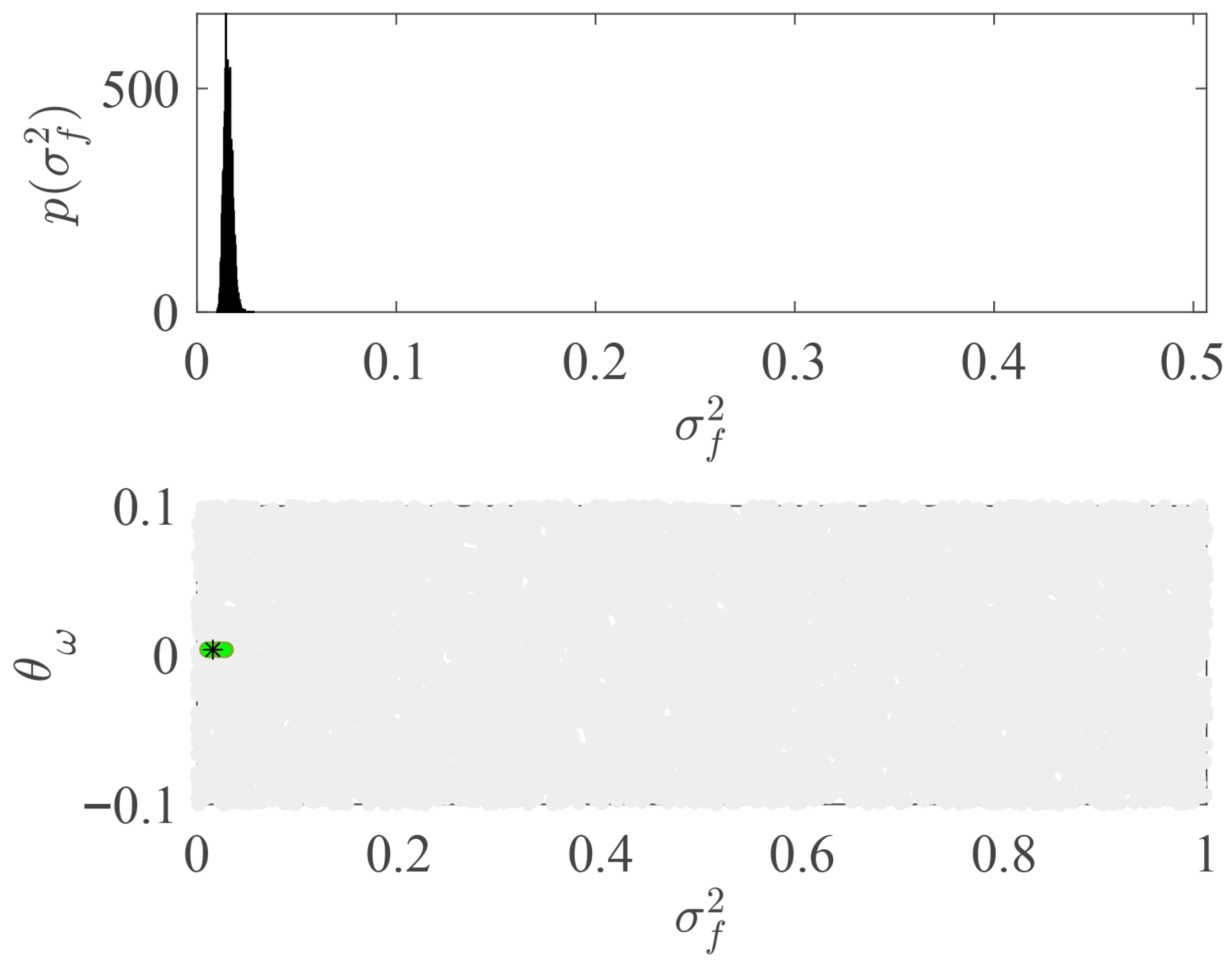
Figure 8 presents the histogram of the frequency prediction error, illustrating the distribution of discrepancies between the predicted and observed dominant frequencies.

3.2. Experimental Case Study

The experimental tests presented in this section are based on the milling setup and data reported in Zorlu et al. [23]. A brief description of the experimental configuration is provided below, and the closed-loop poles identified via OMA in that study are used as inputs to the Bayesian inference framework developed in this work.
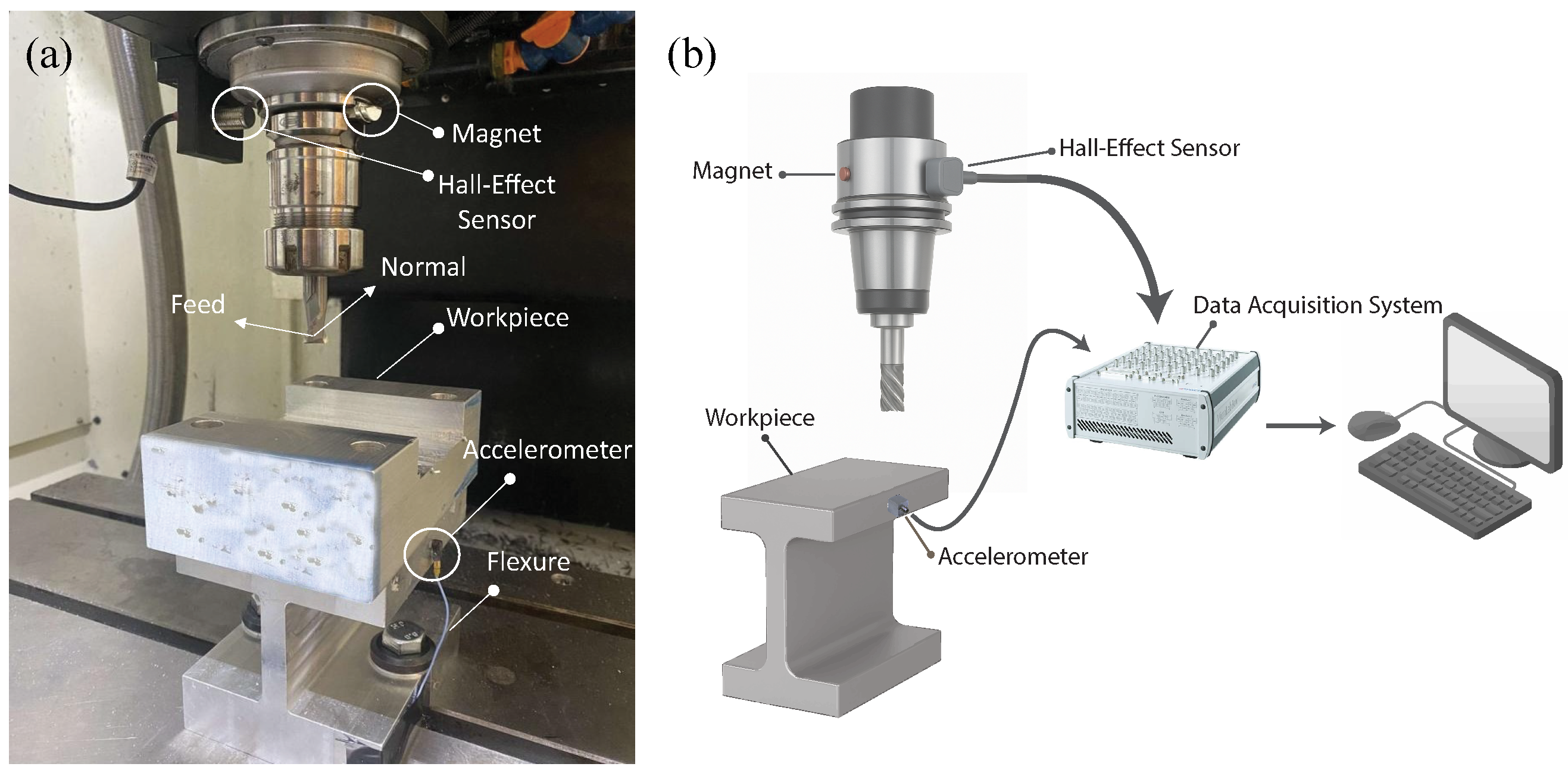
A set of milling tests was conducted using the single-degree-of-freedom milling setup as shown in Figure 9a. The setup consists of a 6061-T6 Aluminum workpiece mounted on a uniaxial compliant fixture, machined by a two-fluted carbide cutting tool with a diameter of 12.7 mm. As shown in Figure 9a, the setup is flexible in the X (feed) direction, and the workpiece is machined using a feedrate of 0.2 mm/tooth in a slotting (full immersion) operation. The tangential and normal linear mechanistic cutting force coefficients were identified by the orthogonal to oblique transformation as K t = 650 MPa and K n = 110 MPa, respectively [40]. The piezoelectric accelerometer (PCB 352C22) is mounted on the flexure in the X-direction. A Hall-effect sensor is used to detect spindle rotation instants and provides the trigger signal for synchronous sampling in dSpace MicroLabBox. Figure 9b illustrates the schematic of the data acquisition setup. This signal provides a precise reference for identifying spindle rotation events and synchronizing the vibration signal with each revolution. Therefore, the accelerometer’s analog signal is sampled at the same tool rotational angles in each period. The number of data points after each trigger is determined by the tooth-passing period and the sampling period. For instance, at 2100 RPM, one full tooth-passing period contains 285 data points when sampled at a rate of 20,000 samples per second.
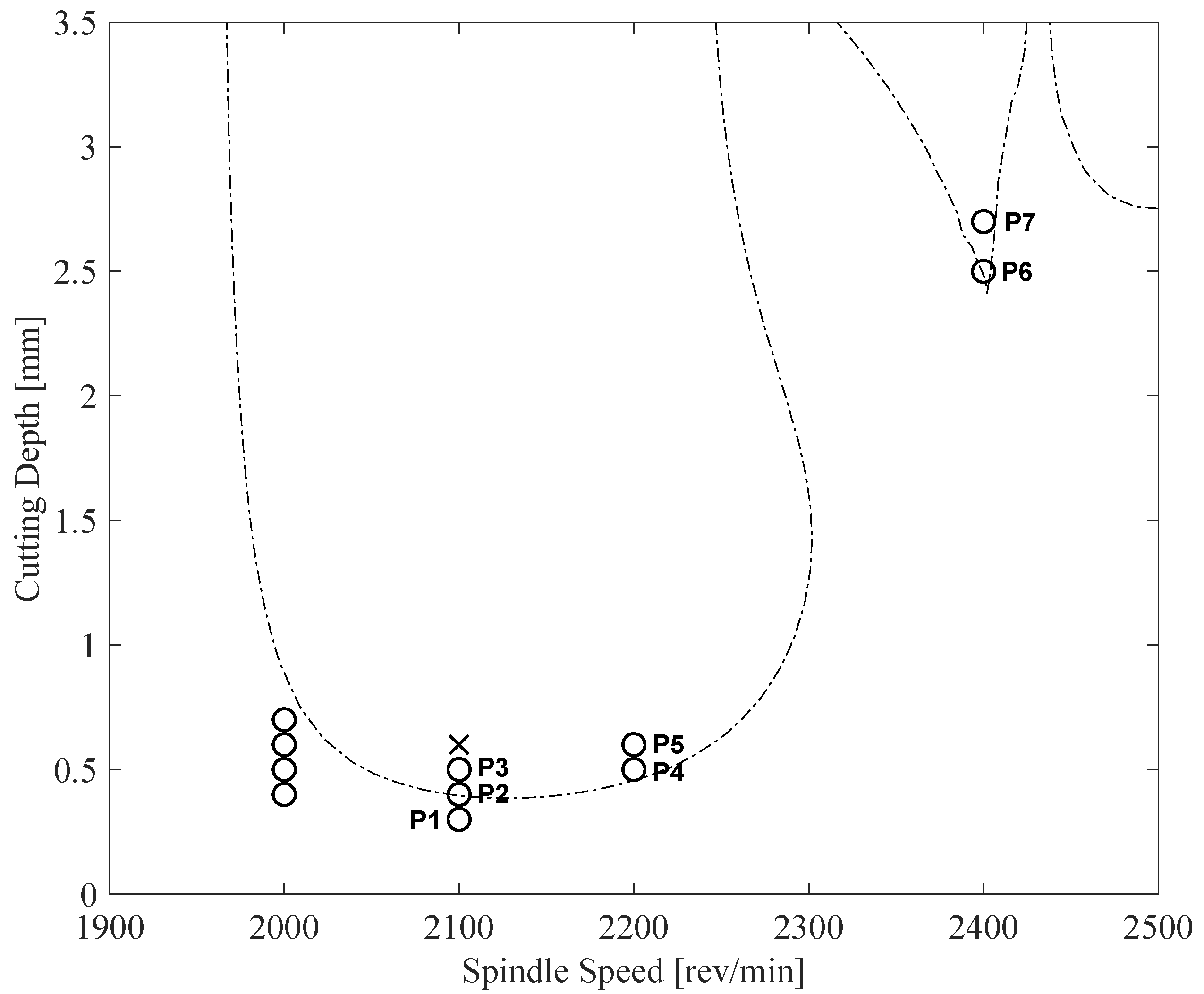
Before removing any material from the workpiece, the modal parameters of the setup in the feed direction are determined by impulse hammer tests as ω n = 2 π × 195.3 rad/s, k x = 2.34 N/ μ m, and ζ x = 0.004 . The stability lobe diagram obtained using the SDM is shown in Figure 10. Also shown in the figure are the experimentally determined stable and unstable points. The proposed OMA was performed for seven of the tested stable points, which are marked as P1 to P7 in the figure.
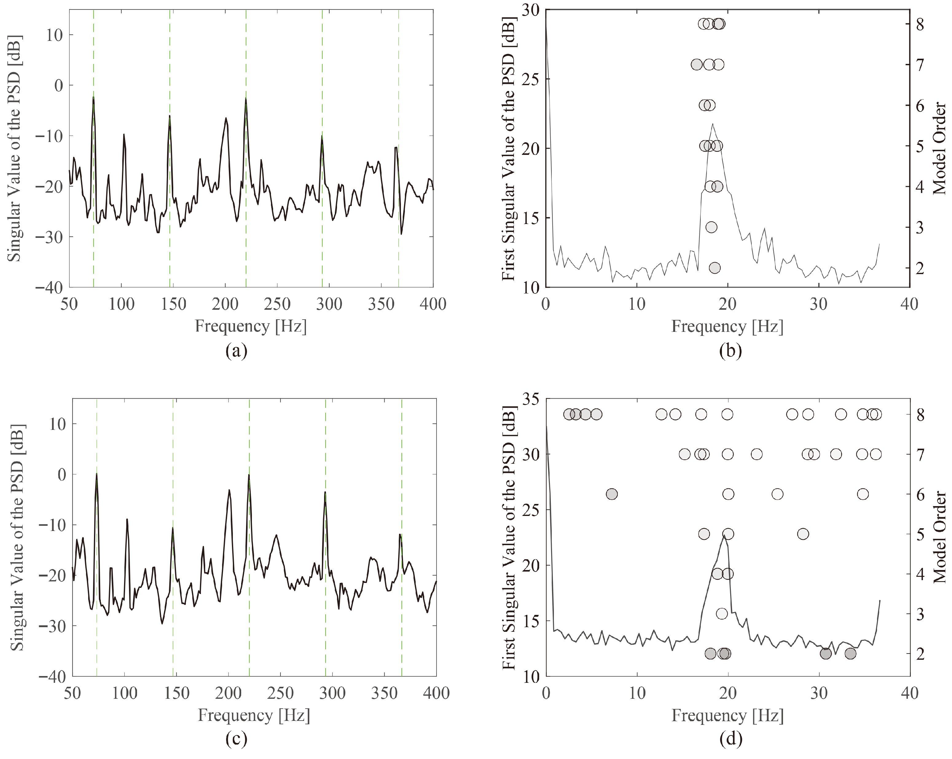
Four sets of full-immersion milling experiments were conducted at spindle speeds between 2000 and 2400 RPM. Figure 11 presents the OMA stabilization diagrams for two representative measurements at 2200 RPM with a 0.5 mm depth of cut (point P4) and 0.6 mm depth of cut (point P5), identified using the TDPR method. More results are reported in ref. [23]. Figure 11a,c is the PSD of the measured machining sound at point P4 and P5, and Figure 11b,d is the corresponding PSD of the lifted vibration signals. In both cases, the vibrations are stable, and the sound spectrum is dominated by harmonics of the tooth-passing frequency. Additionally, the power spectral density (PSD) of the lifted vibration signals exhibits a distinct peak near 20 Hz, which the TDPR method identifies as a stable pole. A similar analysis was performed for all the test conditions ( N p = 7 ) indicated in Figure 10, and the extracted dominant poles are provided in Table 2.
Since each test was repeated multiple times ( N s = 10 ) to ensure consistent results, a substantial amount of material was removed from the workpiece after completing the tests at each cutting pair. This material removal led to a notable change in the system’s modal parameters. As a result, the dominant poles identified by OMA at 2200 and 2400 RPM deviated significantly from the chatter stability predictions based on the SLD constructed using modal parameters obtained from the initial impact hammer test. This discrepancy indicates that the system’s modal parameters evolved during the course of testing, and therefore, they need to be updated to reflect the in-process measurements.
The prior distributions of the modal parameter variations θ m = [ θ ω , θ ζ , θ k ] are assumed to be uniform across [ 0.1 , 0.1 ] for θ ω and θ k , and [ 0.5 , 0.5 ] for θ ζ . The prior distribution of the prediction error variance σ ω 2 is assumed to be uniform across 0 and 1. A training dataset consisting of 3375 different combinations of model parameters was used to construct the GPR model, enabling rapid estimation of the eigenvalues of the monodromy matrix for any given parameter set required by the TMCMC algorithm. The TMCMC generated 5000 samples from the posterior distribution of the parameters based on the assumed priors and the likelihood function. A set of model classes with α k in the range of 0.001 and 1 is considered, and the log marginal likelihood for each α is shown in Figure 12. The model class with α = 0.006 is selected accordingly, and the sampling process is repeated for 10,000 samples according to the selected α .
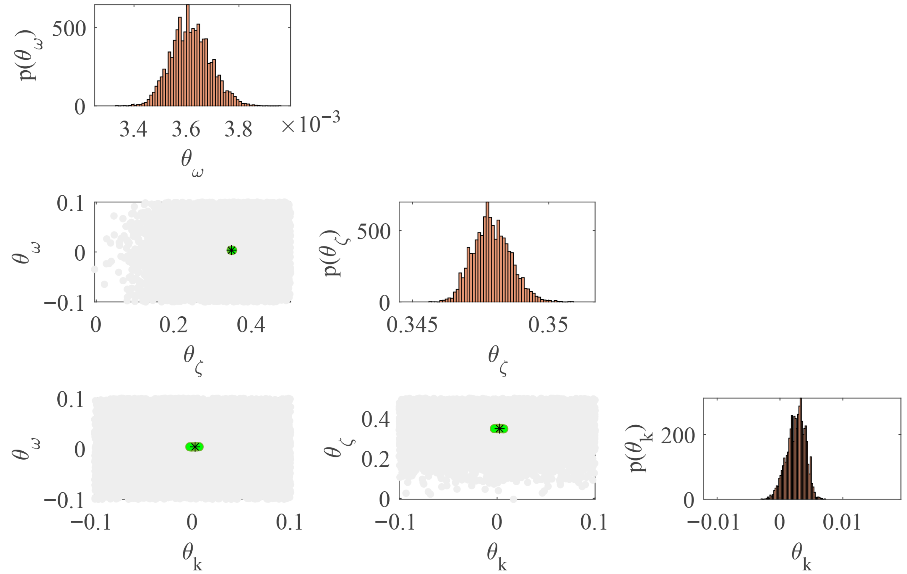
For the selected model class, samples were generated from the posterior distribution of the three model parameters. Figure 13 depicts the joint and marginal distributions of the model parameters θ ω , θ ζ , and θ k used in the Bayesian model updating process. The diagonal plots show the marginal posterior distributions of each parameter, where the histograms indicate high concentration and reduced uncertainty relative to the prior. The off-diagonal plots display the pairwise joint distributions: the gray background points represent the prior samples drawn from uniform distributions, while the green points illustrate the updated posterior samples. In all the off-diagonal plots, the posterior samples cluster tightly, indicating strong parameter identifiability and convergence toward the updated values below. The histogram of the frequency prediction error and its joint distribution with θ ω are shown in Figure 14, further confirming the convergence of the TMCMC algorithm.
  E [ θ ω ,   θ σ ,   θ k ] = [ 3.6 × 10 3 ,   0.35 ,   0.003 ]   Σ θ = 10 6 × 0.005 0.012 0.028 0.012 0.476 0.197 0.028 0.197 2.03
Figure 15 shows samples of the posterior distributions for the same example, except that the prior has a normal distribution for θ with the mean values [ 0 , 0.35 , 0 ] and [ 0.005 , 0.01 , 0.01 ] for variances and a uniform distribution for the prediction error variance, σ ω 2 across 0 and 1.
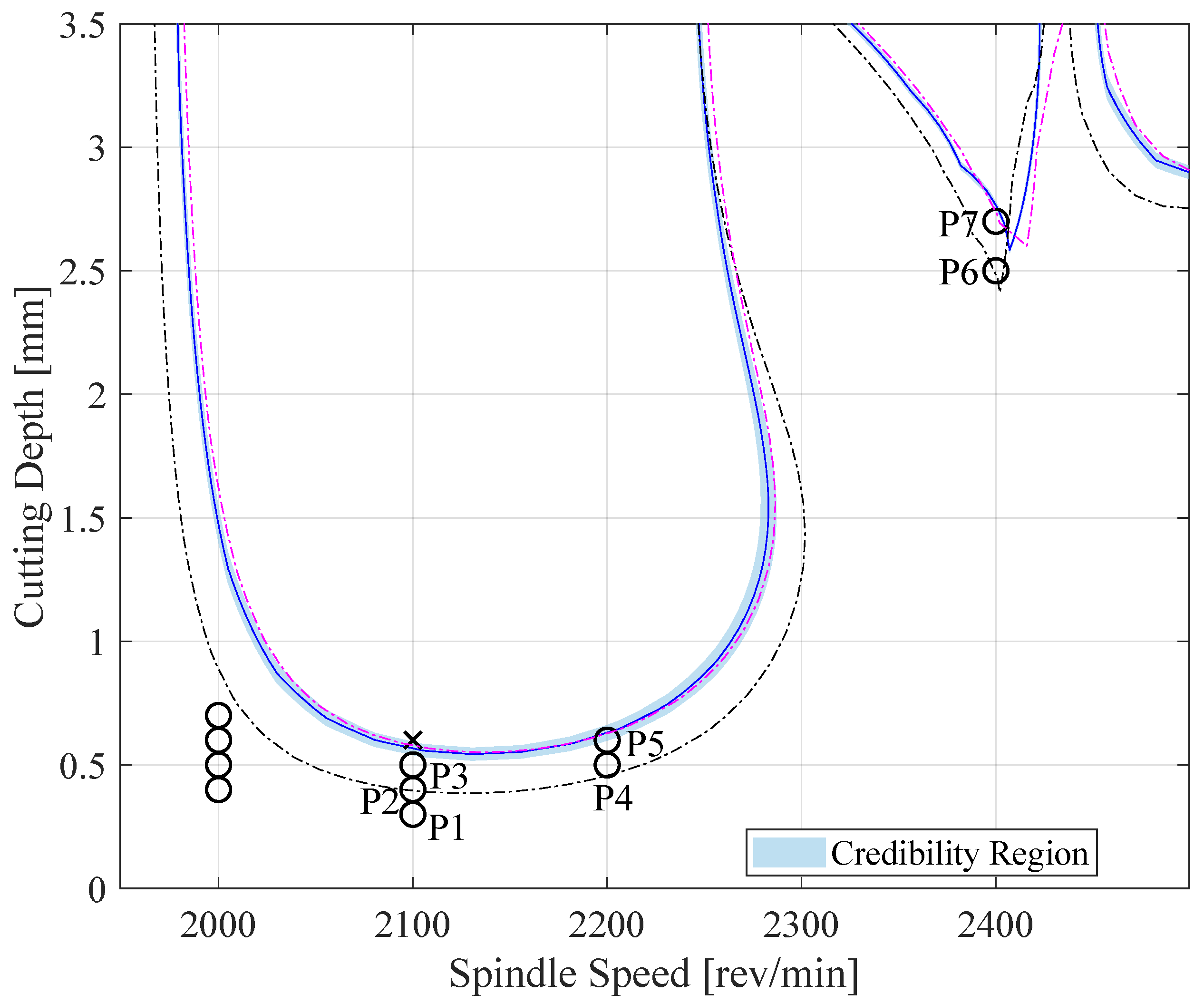
Using the mean values of the updated parameters from Equation (20), the revised SLD is shown in Figure 16, together with its credibility bounds. The upper/lower credibility bounds are obtained from the contour plot of the eigenvalues plus/minus one standard deviation equal to unity. This figure also includes the experimentally determined stable (circles) and unstable (crosses) combinations of spindle speed and axial depth of cut, all of which demonstrate good agreement with the stability boundaries predicted by the updated model. To better illustrate the improvement, it is instructive to compare these results with the initial SLD presented in Figure 10, which was derived from the pre-machining hammer test. While the initial prediction provides a reasonable approximation of the stability limits, its accuracy diminishes as material removal changes the structural dynamics of the workpiece. Specifically, several experimental points near the transition between stable and unstable regions were not well captured by the initial SLD, indicating a shift in the system dynamics that the idle-state hammer test could not account for.
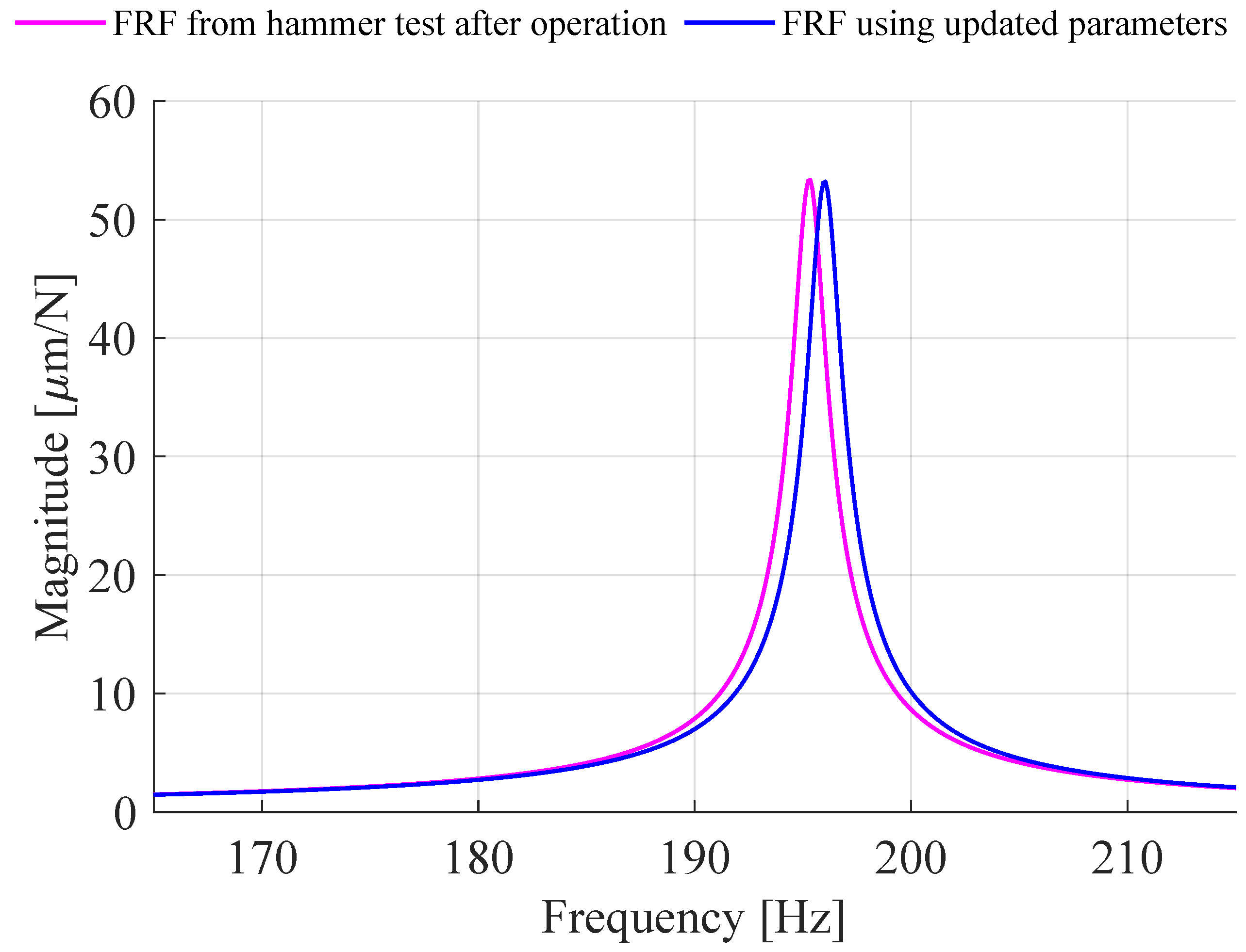
By contrast, the updated SLD in Figure 16 more closely follows the experimentally observed stability behavior. This improvement underscores the capability of the Bayesian updating framework to adapt the underlying system parameters in response to dynamic changes during machining. Notably, the revised stability boundaries align well with the results of the post-process hammer test reported by Zorlu et al. [23]. Figure 17 compares the frequency response function computed from the updated parameters with that obtained through post-process modal testing. The consistency between the updated SLD and both experimental cutting data and post-process modal testing highlights the robustness of the method in accurately tracking shifts in system dynamics.

4. Conclusions

This study applies a Bayesian inference framework to refine the modal parameters of a milling system using in-process vibration data. It addresses a well-known limitation of conventional modal testing, which is typically conducted on idle machines and therefore fails to capture the true dynamics present under operational conditions. This discrepancy often results in inaccurate chatter stability predictions. To overcome this issue, OMA was employed to extract the closed-loop poles of the system from vibration signals measured during stable milling. The experimentally identified poles were then used to update the prior distributions of the system’s modal parameters. An experimental case study demonstrated that the updated parameters improve the accuracy of the stability lobe diagram in comparison with those generated from offline modal testing data.
An important advantage of this approach is its potential to eliminate the need for impact hammer testing. The results of this study show that, even for a uniform prior distribution, which reflects minimal initial knowledge of the system’s dynamics, the Bayesian updating approach can still converge to the true modal parameters using only stable operational data. This makes the method particularly attractive for model calibration in industrial environments, where minimizing manual intervention and reducing experimental effort are critical.
Despite its demonstrated effectiveness, the approach has certain limitations. First, it is not currently applicable for online monitoring or real-time parameter updating, as the process relies on computationally intensive inference. Second, when extended to multi-mode systems, the method results in a high-dimensional parameter space. This is because each additional mode introduces multiple parameters, which significantly increase the computational burden and the complexity of convergence. These factors limit the scalability of the approach for systems with multiple dominant modes.

Author Contributions

Conceptualization, K.A.; methodology, K.A. and A.E.-T.; software, K.A. and A.E.-T.; validation, K.A. and A.E.-T.; formal analysis, A.E.-T.; investigation, A.E.-T.; data curation, A.E.-T.; writing—original draft preparation, A.E.-T.; writing—review and editing, K.A. and A.E.-T.; visualization, A.E.-T.; supervision, K.A.; project administration, K.A.; funding acquisition, K.A. All authors have read and agreed to the published version of the manuscript.

Funding

This research was funded by the Natural Sciences and Engineering Research Council of Canada (NSERC), grant number RGPIN-2025-06423.

Data Availability Statement

The datasets generated and analyzed during the current study are available from the authors upon reasonable request.

Conflicts of Interest

The authors declare no conflict of interest.

References

  1. Tobias, S.A. Machine Tool Vibration; Blackie and Sons Ltd.: Glasgow, UK, 1965. [Google Scholar]
  2. Munoa, J.; Beudaert, X.; Dombovari, Z.; Altintas, Y.; Budak, E.; Brecher, C.; Stepan, G. Chatter suppression techniques in metal cutting. CIRP Ann. 2016, 65, 785–808. [Google Scholar] [CrossRef]
  3. Quintana, G.; Ciurana, J. Chatter in machining processes: A review. Int. J. Mach. Tools Manuf. 2011, 51, 363–376. [Google Scholar] [CrossRef]
  4. Altintas, Y.; Stepan, G.; Budak, E.; Schmitz, T.; Kilic, Z.M. Chatter Stability of Machining Operations. J. Manuf. Sci. Eng. 2020, 142, 110801. [Google Scholar] [CrossRef]
  5. Iglesias, A.; Taner Tunç, L.; Özsahin, O.; Franco, O.; Munoa, J.; Budak, E. Alternative experimental methods for machine tool dynamics identification: A review. Mech. Syst. Signal Process. 2022, 170, 108837. [Google Scholar] [CrossRef]
  6. Suzuki, N.; Kurata, Y.; Kato, T.; Hino, R.; Shamoto, E. Identification of transfer function by inverse analysis of self-excited chatter vibration in milling operations. Precis. Eng. 2012, 36, 568–575. [Google Scholar] [CrossRef]
  7. Özşahin, O.; Budak, E.; Özgüven, H. In-process tool point FRF identification under operational conditions using inverse stability solution. Int. J. Mach. Tools Manuf. 2015, 89, 64–73. [Google Scholar] [CrossRef]
  8. Grossi, N.; Sallese, L.; Scippa, A.; Campatelli, G. Improved experimental-analytical approach to compute speed-varying tool-tip FRF. Precis. Eng. 2017, 48, 114–122. [Google Scholar] [CrossRef]
  9. Postel, M.; Özsahin, O.; Altintas, Y. High speed tooltip FRF predictions of arbitrary tool-holder combinations based on operational spindle identification. Int. J. Mach. Tools Manuf. 2018, 129, 48–60. [Google Scholar] [CrossRef]
  10. Eynian, M. In-process identification of modal parameters using dimensionless relationships in milling chatter. Int. J. Mach. Tools Manuf. 2019, 143, 49–62. [Google Scholar] [CrossRef]
  11. Karandikar, J.; Traverso, M.; Abbas, A.; Schmitz, T. Bayesian Inference for Milling Stability Using a Random Walk Approach. J. Manuf. Sci. Eng. 2014, 136, 031015. [Google Scholar] [CrossRef]
  12. Karandikar, J.; Honeycutt, A.; Schmitz, T.; Smith, S. Stability boundary and optimal operating parameter identification in milling using Bayesian learning. J. Manuf. Process. 2020, 56, 1252–1262. [Google Scholar] [CrossRef]
  13. Rahimi, M.H.; Huynh, H.N.; Altintas, Y. On-line chatter detection in milling with hybrid machine learning and physics-based model. CIRP J. Manuf. Sci. Technol. 2021, 35, 25–40. [Google Scholar] [CrossRef]
  14. Postel, M.; Bugdayci, B.; Wegener, K. Ensemble transfer learning for refining stability predictions in milling using experimental stability states. Int. J. Adv. Manuf. Technol. 2020, 107, 4123–4139. [Google Scholar] [CrossRef]
  15. Wiederkehr, P.; Finkeldey, F.; Siebrecht, T. Reduction of experimental efforts for predicting milling stability affected by concept drift using transfer learning on multiple machine tools. CIRP Ann. 2024, 73, 301–304. [Google Scholar] [CrossRef]
  16. Minis, I.E.; Magrab, E.B.; Pandelidis, I.O. Improved Methods for the Prediction of Chatter in Turning, Part 1: Determination of Structural Response Parameters. J. Eng. Ind. 1990, 112, 12–20. [Google Scholar] [CrossRef]
  17. Özşahin, O.; Budak, E.; Özgüven, H. Investigating Dynamics of Machine Tool Spindles under Operational Conditions. Adv. Mater. Res. 2011, 223, 610–621. [Google Scholar] [CrossRef]
  18. Rudel, V.; Kienast, P.; Vinogradov, G.; Ganser, P.; Bergs, T. Cloud-based process design in a digital twin framework with integrated and coupled technology models for blisk milling. Front. Manuf. Technol. 2022, 2, 1021029. [Google Scholar] [CrossRef]
  19. Brincker, R. Introduction to Operational Modal Analysis; John Wiley & Sons: London, UK, 2015. [Google Scholar]
  20. Berthold, J.; Kolouch, M.; Regel, J.; Putz, M. Investigation of the Dynamic Behavior of Machine Tools During Cutting by Operational Modal Analysis. MM Sci. J. 2019, 2019, 3078–3085. [Google Scholar] [CrossRef]
  21. Kim, S.; Ahmadi, K. Estimation of vibration stability in turning using operational modal analysis. Mech. Syst. Signal Process. 2019, 130, 315–332. [Google Scholar] [CrossRef]
  22. Ebrahimi-Tirtashi, A.; Ahmadi, K. Automated Operational Modal Analysis of Self-Excited Vibrations in Turning. Mech. Syst. Signal Process. 2025, 233, 112705. [Google Scholar] [CrossRef]
  23. Zorlu, A.; Ahmadi, K.; Ebrahimi-Tirtashi, A. Operational Modal Analysis of Self-Excited Vibrations in Milling Considering Periodic Dynamics. J. Manuf. Sci. Eng. 2025, 147, 021010. [Google Scholar] [CrossRef]
  24. Beck, J.L.; Katafygiotis, L.S. Updating Models and Their Uncertainties. I: Bayesian Statistical Framework. J. Eng. Mech. 1998, 124, 455–461. [Google Scholar] [CrossRef]
  25. Beck, J.L. Bayesian system identification based on probability logic. Struct. Control Health Monit. 2010, 17, 825–847. [Google Scholar] [CrossRef]
  26. Goller, B.; Beck, J.; Schueller, G. Evidence-based identification of weighting factors in Bayesian model updating using modal data. J. Eng. Mech. 2012, 138, 430–440. [Google Scholar] [CrossRef]
  27. Ahmadi, K. Bayesian updating of modal parameters for modeling chatter in turning. CIRP J. Manuf. Sci. Technol. 2022, 38, 724–736. [Google Scholar] [CrossRef]
  28. Insperger, T.; Mann, B.; Stépán, G.; Bayly, P. Stability of up-milling and down-milling, part 1: Alternative analytical methods. Int. J. Mach. Tools Manuf. 2003, 43, 25–34. [Google Scholar] [CrossRef]
  29. Insperger, T.; Stépán, G. Updated semi-discretization method for periodic delay-differential equations with discrete delay. Int. J. Numer. Methods Eng. 2004, 61, 117–141. [Google Scholar] [CrossRef]
  30. Altintaş, Y.; Budak, E. Analytical Prediction of Stability Lobes in Milling. CIRP Ann. 1995, 44, 357–362. [Google Scholar] [CrossRef]
  31. Allen, M.S.; Sracic, M.W.; Chauhan, S.; Hansen, M.H. Output-only modal analysis of linear time-periodic systems with application to wind turbine simulation data. Mech. Syst. Signal Process. 2011, 25, 1174–1191. [Google Scholar] [CrossRef]
  32. Bamieh, B.; Pearson, J.B.; Francis, B.A.; Tannenbaum, A. A lifting technique for linear periodic systems with applications to sampled-data control. Syst. Control. Lett. 1991, 17, 79–88. [Google Scholar] [CrossRef]
  33. Chib, S.; Jeliazkov, I. Marginal Likelihood From the Metropolis–Hastings Output. J. Am. Stat. Assoc. 2001, 96, 270–281. [Google Scholar] [CrossRef]
  34. Friel, N.; Pettitt, A.N. Marginal Likelihood Estimation via Power Posteriors. J. R. Stat. Soc. Ser. B Stat. Methodol. 2008, 70, 589–607. [Google Scholar] [CrossRef]
  35. Betz, W.; Papaioannou, I.; Straub, D. Transitional Markov Chain Monte Carlo: Observations and Improvements. J. Eng. Mech. 2016, 142, 04016016. [Google Scholar] [CrossRef]
  36. Ching, J.; Chen, Y.C. Transitional Markov Chain Monte Carlo Method for Bayesian Model Updating, Model Class Selection, and Model Averaging. J. Eng. Mech. 2007, 133, 816–832. [Google Scholar] [CrossRef]
  37. Nobari, A.; Ouyang, H.; Bannister, P. Statistics of complex eigenvalues in friction-induced vibration. J. Sound Vib. 2015, 338, 169–183. [Google Scholar] [CrossRef]
  38. Rasmussen, C.E. Gaussian Processes in Machine Learning. In Summer School on Machine Learning; Notes in Computer Science; Springer: Berlin, Germany, 2003; pp. 63–71. [Google Scholar]
  39. Insperger, T.; Stépán, G.; Bayly, P.; Mann, B. Multiple chatter frequencies in milling processes. J. Sound Vib. 2003, 262, 333–345. [Google Scholar] [CrossRef]
  40. Budak, E.; Altintas, Y.; Armarego, E.J.A. Prediction of Milling Force Coefficients From Orthogonal Cutting Data. J. Manuf. Sci. Eng. 1996, 118, 216–224. [Google Scholar] [CrossRef]
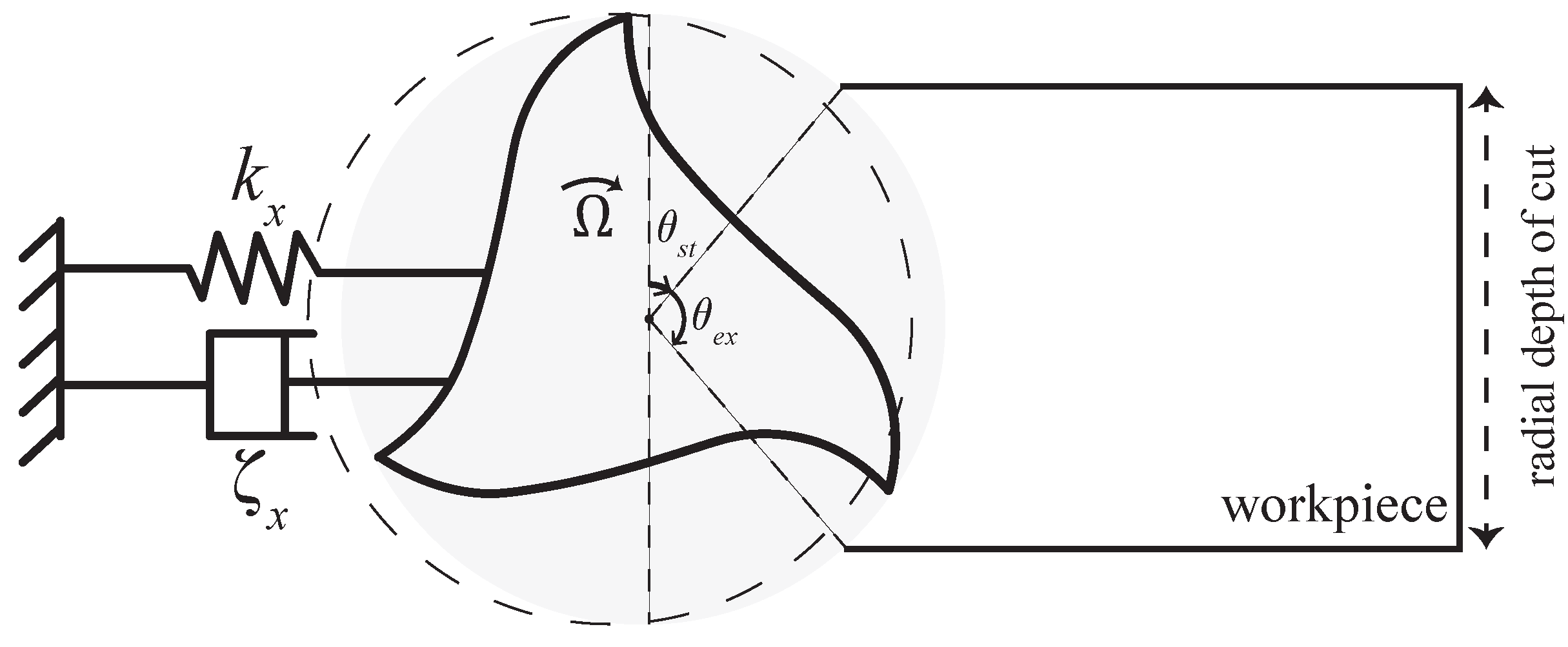
Figure 1. SDOF model of milling process.
Jmmp 09 00323 g001
Figure 2. Block diagram of the SDOF numerical simulations of the self-excited vibration in milling.
Jmmp 09 00323 g002
Figure 3. Stability lobe diagram of the numerical simulation; circles and crosses are stable and unstable points, respectively.
Jmmp 09 00323 g003
Figure 4. PSD of the vibrations at 2100 RPM and 0.4 mm depth of cut. Tooth-passing frequency harmonics are indicated by dashed lines.
Jmmp 09 00323 g004
Figure 5. Stabilizationdiagram of the lifted response at 2100 RPM and 0.4 mm depth of cut plotted on the first singular values of the PSD matrix. The shading of the circles corresponds to the damping ratio of the poles.
Jmmp 09 00323 g005
Figure 6. Model evidence (log marginal likelihood) for different amounts of α in the numerical simulation.
Jmmp 09 00323 g006
Figure 7. Samples from uniform prior (gray points) and updated posterior (green points) distributions of model parameters in the numerical simulation. (*) indicates the centroid of the samples from the posterior distribution.
Jmmp 09 00323 g007
Figure 8. Samples from uniform prior (gray points) and updated posterior (green points) distributions of prediction error in the numerical simulation. (*) indicates the centroid of the samples from the posterior distribution.
Jmmp 09 00323 g008
Figure 9. (a) The experimental setup [23]. (b) Setup configuration for the data acquisition.
Jmmp 09 00323 g009
Figure 10. Stability lobe diagrams based on impact hammer test results before milling process; circles and crosses are experimentally determined stable and unstable points, respectively.
Jmmp 09 00323 g010
Figure 11. PSD of the machining sound (a,c) and stabilization diagrams (b,d) for 0.5 mm and 0.6 mm depths of cut at 2200 RPM, respectively. Tooth-passing frequency harmonics are indicated by dashed lines, and the shading of the circles corresponds to the damping ratio of the poles.
Jmmp 09 00323 g011
Figure 12. Model evidence (log marginal likelihood) for different amounts of α in the experimental case study.
Jmmp 09 00323 g012
Figure 13. Samples from uniform prior (gray points) and updated posterior (green points) distributions of model parameters. (*) indicates the centroid of the samples from the posterior distribution.
Jmmp 09 00323 g013
Figure 14. Samples from uniform prior (gray points) and updated posterior (green points) distributions of prediction error. (*) indicates the centroid of the samples from the posterior distribution.
Jmmp 09 00323 g014
Figure 15. Samples from normal prior (gray points) and updated posterior (green points) distributions of model parameters. (*) indicates the centroid of the samples from the posterior distribution.
Jmmp 09 00323 g015
Figure 16. Stability lobe diagrams. Jmmp 09 00323 i001: Initial SLD using parameters obtained by an impact hammer test before starting the milling operations.Jmmp 09 00323 i002: Updated SLD using mean of posterior. Jmmp 09 00323 i003: SLD using parameters obtained by an impact hammer test after operations [23]. Circles and crosses are experimentally determined stable and unstable points, respectively. P1–P7 are the stable points used in model updating.
Jmmp 09 00323 g016
Figure 17. Frequency response function.
Jmmp 09 00323 g017
Table 1. Dominant closed-loop poles identified by TDPR at 7 spindle speed and cutting depth combinations in the numerical simulation.
pSpindle Speed
[RPM]
Cutting Depth
[mm]
ω ^ p
[Hz]
ζ ^ p
120000.4 4.69 ± 0.0182 0.088 ± 0.0143
220000.5 4.6 ± 0.0222 0.0722 ± 0.0157
320000.6 4.56 ± 0.0362 0.0501 ± 0.0133
420000.7 4.53 ± 0.0233 0.0303 ± 0.0066
520000.8 4.45 ± 0.0889 0.01 ± 0.0047
621000.3 14.14 ± 0.0102 0.03 ± 0.0063
721000.4 14.05 ± 0.0041 0.0129 ± 0.0037
Table 2. Dominant closed-loop poles identified by TDPR at 7 spindle speed and cutting depth combinations in the experimental case study.
pSpindle Speed
[RPM]
Cutting Depth
[mm]
ω ^ p
[Hz]
ζ ^ p
121000.3 10.6 ± 0.09 0.088 ± 0.025
221000.4 11.2 ± 0.01 0.0722 ± 0.012
321000.5 11.5 ± 0.01 0.0501 ± 0.015
422000.5 19.7 ± 0.0233 0.01 ± 0.005
522000.6 19.9 ± 0.0889 0.003 ± 0.001
624002.5 39.9 ± 0.0102 0.02 ± 0.006
724002.7 40 ± 0.0041 0.0005 ± 0.0002
Disclaimer/Publisher’s Note: The statements, opinions and data contained in all publications are solely those of the individual author(s) and contributor(s) and not of MDPI and/or the editor(s). MDPI and/or the editor(s) disclaim responsibility for any injury to people or property resulting from any ideas, methods, instructions or products referred to in the content.