Abstract
The real-time, full-field simulation of the tube hydroforming process is crucial for deformation monitoring and the timely prediction of defects. However, this is rather difficult for finite-element simulation due to its time-consuming nature. To overcome this drawback, in this paper, a surrogate model framework was proposed by integrating the finite-element method (FEM) and machine learning (ML), in which the basic methodology involved interrupting the computational workflow of the FEM and reassembling it with ML. Specifically, the displacement field, as the primary unknown quantity to be solved using the FEM, was mapped onto the displacement boundary conditions of the tube component with ML. To this end, the titanium tube material as well as the hydroforming process was investigated, and a fairly accurate FEM model was developed based on the CPB06 yield criterion coupled with a simplified Kim–Tuan hardening model. Numerous FEM simulations were performed by varying the loading conditions to generate the training database for ML. Then, a random forest algorithm was applied and trained to develop the surrogate model, in which the grid search method was employed to obtain the optimal combination of the hyperparameters. Sequentially, the principal strain, the effective strain/stress, as well as the wall thickness was derived according to continuum mechanics theories. Although further improvements were required in certain aspects, the developed FEM-ML surrogate model delivered extraordinary accuracy and instantaneity in reproducing multi-physical fields, especially the displacement field and wall-thickness distribution, manifesting its feasibility in the real-time, full-field simulation and monitoring of deformation states.
1. Introduction
Tube hydroforming is a long-established and important metal forming technology that is widely applied across many industrial fields [1,2,3,4], in which the tubes are forced to conform to a die shape by fluid pressure and axial forces simultaneously [1,5]. Such forming features offer many advantages over other manufacturing approaches, including weight reduction, part consolidation, reduced scrap, improved mechanical properties, etc. [3]. However, the hydroforming process also suffers from some inherent problems such as wrinkling, fracture, bursting, etc. [3,4]. As the quality of the hydroforming parts is strongly dependent on the processing conditions, the optimum load sequencing should be carefully selected prior to forming. Thereinto, the finite-element method (FEM) has been proved to be, probably, the most powerful tool to predict tube deformation and optimize the process parameters, whereby the lengthy and expensive trial-and-error forming experiments can be avoided [1,4,6,7]. However, the FEM analysis, which is generally performed in an offline manner, seems to be very idealistic, since it oversimplifies the forming processes, especially the boundary conditions. Unexpected failure may occur even when using the pre-optimized processing routes in hydroforming, which is probably due to the fluctuation of the loading parameters, as well as the unpredictable material defects [8]. Such an issue becomes increasingly prominent for the process of high special strength materials with lower formability and higher flow resistance, as these materials are generally stressed to their maximum formability [9]. Moreover, the tube blank is closely sealed in the die during the entire hydroforming process, such that its deformation state cannot be directly observed or detected. Therefore, an online or real-time FEM analysis, which is driven by the practical loading parameters and capable of predicting the deformation synchronously with the actual process, is of particular significance for tube hydroforming. On one hand, the online FEM provides the continuous monitoring of an otherwise not observable deformation state and forming quality; on the other hand, it offers the basis for the active controlling of the forming process by visualizing the interrelationship between processing conditions and internal physical fields.
Apparently, achieving a real-time deformation prediction requires that the FEM is capable of instant response that permits it to keep pace with the actual forming process. Meanwhile, plastic deformation is a highly nonlinear problem involving geometric nonlinearity, material nonlinearity, and contact nonlinearity, which are mathematically modelled by a set of complex partial differential equations (PDEs) that cannot be solved analytically [10]. In general, the FEM solves PDEs by numerical integration technologies either implicitly or explicitly [11]. The implicit integration requires extensive iterations to achieve the global equilibrium requirement within every incremental step, while the explicit approach is based on the central difference method and needs very small time increments to ensure the accuracy of the integration. Therefore, the FEM is essentially time-consuming and computationally expensive to address the plastic problems, and hence seems unfeasible in real-time predictions.
In recent years, machine learning (ML) has gained significant momentum in materials science and solid mechanics [12,13,14,15]. The fundamental concept of the ML framework inferring from the training data consists of a surrogate model with predictive capacity, enabling it to learn complex, nonlinear mappings from a high-dimensional feature vector to a desired output, but without any mathematical algorithm or physical background [16,17]. Therefore, ML models are capable of notably rapid inferences, which may be feasible for real-time prediction in conjunction with the FEM. That is, the offline FEM can be employed as a dataset generator to produce quantities of high-fidelity training data for ML; then, a surrogate model can be developed, which offers instant feedback once the input data are passed through. In a very recent study, Neubürger et al. have developed a digital sensor prototype through the FEM and ML to virtually predict the temperature evolution of a manganese–boron steel blank during press-hardening [18]. The authors generated 20,412 FEM simulation runs by varying the processing parameters to calculate the possible temperature fields, and the ML models were developed to map the nonlinear heat transfer from the blank to the die. The digital sensor was demonstrated to be able to accurately estimate the blank temperature at any time in the press-hardening process. Similar works have been conducted by Ye et al. [19,20], who designed an ML-based model to predict the real-time vertical displacement of steel roof truss structures under different fire scenarios. The FEM and CFD (computational fluid dynamics) analyses were performed for data generation, and the ML models were developed to interrelate the temperatures and displacements at critical positions of the structures. The developed ML model as a digital sensor demonstrates its feasibility in providing timely and reliable monitoring of structural safety.
The literature review manifests that FEM-ML technologies have been attracting increasing attention to address nonlinear plastic problems. Decades earlier, an artificial neural network (ANN) was utilized as a typical ML algorithm to describe the high temperature flow strength of metallic materials, considering the complex effects of strain, strain rate, and temperature [21,22,23,24], which generally showed perfect agreement with experimental flow curves. Despite the intricate input–output relationships, such a straightforward mapping from deformation conditions to flow strengths is somewhat superficial as it neglects the effect of deformation history. More recently, researchers gradually noted the tremendous abilities of ML, especially the sequence learning models, in capturing the mechanical responses accounting for substantial time or path dependencies [17,25,26,27,28,29,30,31]. This essentially facilities the implementation of ML-type constitutive frameworks into FEM codes to replace the traditional models with over-complicated mathematical forms [9,17,32,33]. Particularly, by integrating the crystal plasticity FEM (CPFEM), ML modelling, and macroscale FEM simulation, cross-scale deformation prediction can be achieved [34,35,36]. Thereinto, the CPFEM, which is computationally expensive but can accurately capture the mechanical response by considering crystal rotation and deformation heterogeneities, is applied to generate the training database for ML modelling. Then, the obtained surrogate model can provide the instant constitutive response that is requested by the integration points of the macroscale FEM model. In addition, the FEM-ML approach has also emerged as a feasible and efficient alternative to solve the inverse plastic problems [9,37]. The common framework is that a load-displacement database is generated from the results of the parametric studies of the FEM simulation, based on which the ML models are trained and employed to convert the experimental load-displacement curves (currently, this mainly refers to load–depth curves via instrumented indentation or nanoindentation) into meaningful hardening parameters [38].
Even though the FEM-ML approach constitutes a powerful tool to bring ground-breaking innovations for dealing with nonlinear plastic problems, its application to the real-time, full-field simulation of the plastic forming process has rarely arose until now. The major challenge is that the materials generally undergo a highly inhomogeneous and ever-changing flow during forming. The extremely complicated deformation history is quite difficult to describe with ML due to its physics-free nature. Nevertheless, in the current study, we seek to develop an FEM-ML model framework for a specific tube hydroforming process, where the methodological foundation involves interrupting the numerical workflow of the FEM and resembling it with ML according to the continuum mechanics theory. The developed surrogate model can instantly predict the evolution of the multi-physical fields in the entire forming process with high accuracy, which could be of significance in monitoring the quality problem and process controlling.
The present work is structured as follows. In Section 2, we provide the experimental details and results for tube material characterization and the hydroforming process, based on which the FEM model is developed in Section 3. After that, the methodology and framework of the FEM-ML-based model is described in Section 4, as well as the validation of the model. In Section 5, the developed surrogate model is discussed in terms of deficiencies and limitations, and the work ends with a conclusion in Section 6.
2. Experiments and Results
2.1. Tube Material Characterization
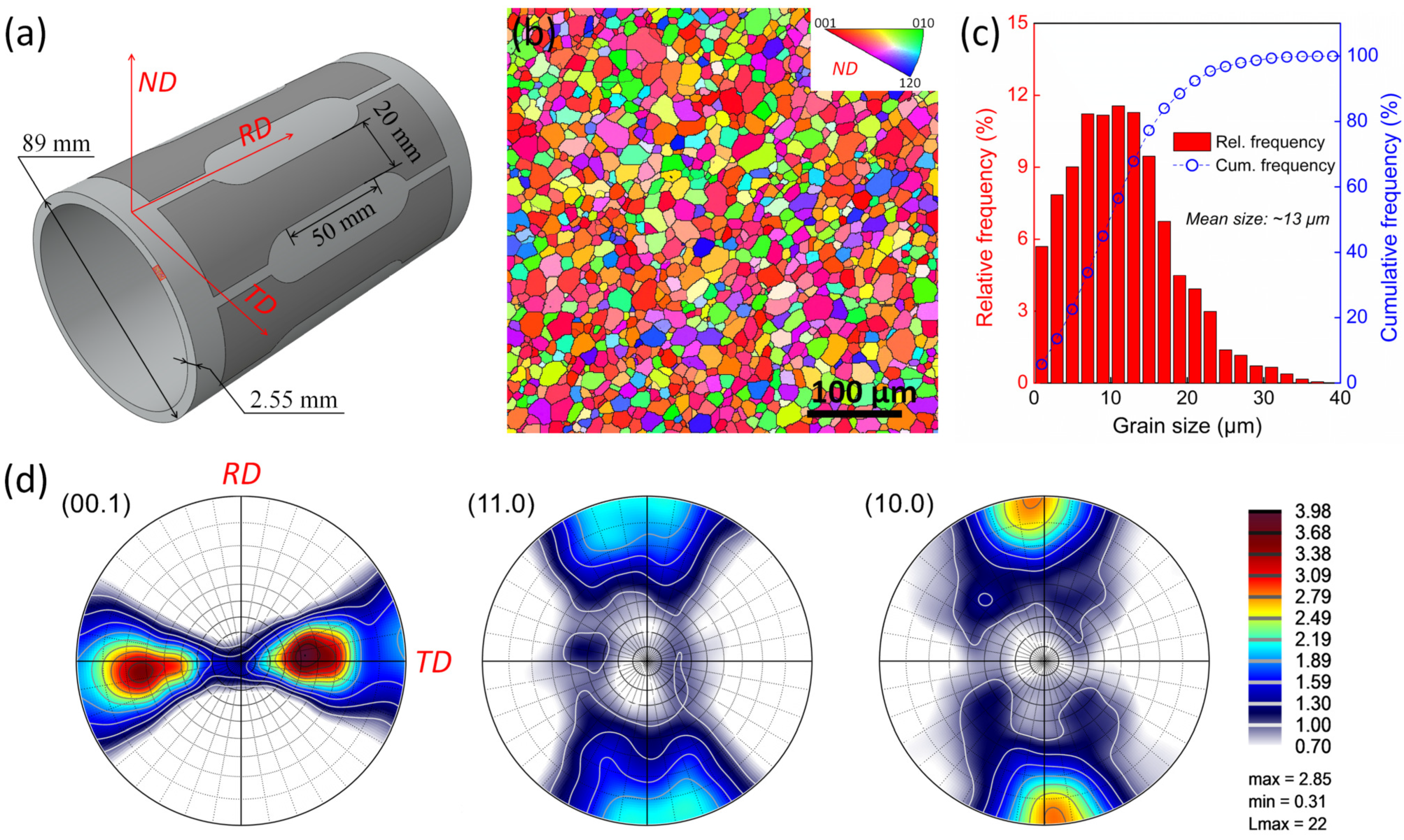
The tubular material applied in the present study is Grade 2 commercial pure titanium (CP-Ti), and the chemical composition measured is tubulated in Table 1. The tube was fabricated by hot rolling followed by recrystallization annealing. The outer diameter is 89 mm with a wall thickness of ~2.55 mm, as depicted in Figure 1a. To characterize the microstructure, the metallographic specimen was machined from the tube, and the cross-section (i.e., the ND-TD plane where TD is the tangent direction and ND denotes the normal direction, as shown in Figure 1a) was mechanically ground and polished with oxide polishing suspension (OPS). EBSD (electron backscattered diffraction) analysis was performed on the polished surface by employing a Zeiss-Sigma500 scanning electron microscope (SEM, Carl Zeiss AG). The accelerating voltage utilized was 20 kV with a stepping size of 1 μm. The EBSD data were analyzed by using the ATEX software (version 4.14) [39]. As shown in Figure 1b,c, the microstructure consists of full-recrystallized, fine, and equiaxed α grains with a mean grain size of ~13 μm. Meanwhile, the pole figures shown in Figure 1d demonstrate that the tube material exhibits a tilted basal texture that splits and orientates away from ND toward TD. Such a texture component is the same with that of the hot-rolled plates [40,41,42], assuming that the tube is flattened. This implies that the tube may possess similar plastic anisotropy characteristics with those of the rolled plates.

Table 1.
Chemical composition of the Grade 2 CP-Ti.

Figure 1.
(a) Schematic description of the tubular blank and the dimension. ND, RD, and TD denote normal direction, rolling direction, and tangent direction, respectively. (b) Inverse-pole-figure map of the tube material. (c) Histogram of grain size distribution. (d) Pole figures to show the texture components of the material.
Tensile tests were performed in order to characterize the mechanical properties. As seen in Figure 1a, longitudinal specimens with a gauge dimension of 50 mm × 20 mm × 2.55 mm were machined from the tube with their axis along RD. The tensile tests were conducted on an MTS universal testing machine equipped with a LaserXtens extensometer and a digital image correlation (DIC) system. The testing started with a loading speed of 1 mm/min prior to yielding, and then switched to 5 mm/min until the rupture of the specimens.
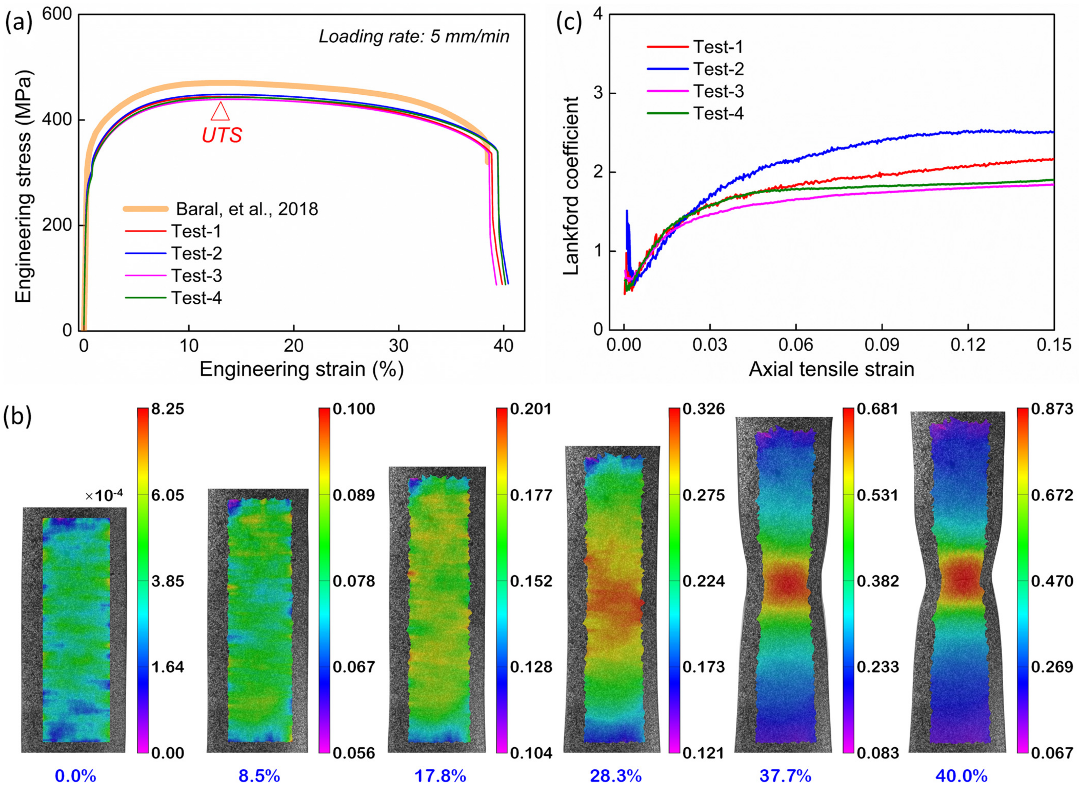
The obtained engineering stress–strain curves of four repeated tests are plotted in Figure 2a, and a good repeatability is noted. One can observe that the material is quite ductile with a rapture elongation of nearly 40%. However, the maximum stress point corresponding to the ultimate tensile strength (UTS) appears very early (at a strain of ~13% as marked in the figure), followed by a sluggish descending of the curves. This indicates an exceedingly retarded necking behavior due to the distinct distortional hardening of titanium [43,44,45], which is also confirmed by the sample profiles captured with DIC during tension, as seen in Figure 2b. Meanwhile, the measured axial and transverse strain fields captured with DIC are used to determine the evolution of the Lankford coefficient (i.e., R-value) which can reflect the plastic anisotropy. According to the definition, the Lankford coefficient is the ratio of the width-to-thickness strain increments. As seen in Figure 2c, the coefficient curves are gradually increased to be about 2 at an axial strain of ~0.06, and then they are roughly kept constant. The high Lankford coefficients imply a strong plastic anisotropy of the present material.

Figure 2.
(a) Stress–strain curves obtained from four repeated tensile tests along RD. The tensile curve quoted from [45] is also superimposed for comparison. (b) DIC images showing the evolution of the axial strain distribution during tension. (c) Lankford coefficient curves derived from the DIC results.
It should be mentioned that to date, Baral et al. [45,46] have performed one of the most systematic studies on the plastic anisotropy of Grade 2 CP-Ti-rolled plates, and the tensile curve they obtained is only slightly derived from the present one by ~25 MPa (Figure 2a). Both the strain hardening histories and the rupture elongations are nearly identical. Meanwhile, the Lankford coefficients are also fairly close. All these observations imply that the present tube material possesses an identical plastic anisotropy with that of the CP-Ti plates studied by Baral et al. [45,46].
2.2. Tube Hydroforming Procedure
The tubular blanks with a length of 316 mm were applied to fabricate tee-shaped joints. The principle of the hydroforming process is schematically shown in Figure 3a. The tubular blank is placed between two contoured die halves and then filled with hydraulic oil through holes in the seal punches. The tube is then forced to adopt the inner contour of the tool under the simultaneously controlled action of the internal pressure and the axial displacements of the two seal punches. To minimize the friction, molybdenum disulfide powder is utilized as lubricant. Meanwhile, the counterpressure punch, which exerts a constant pressure of 0.2 MPa on the top of the tube branch, is forced to move back during hydroforming. The commonly used loading path is shown in Figure 3b, along with the loading parameters. When the residual length of the tubular component reached 244 mm, the processing was stopped to take out the component. The total height of the tee-branch as well as the wall-thickness of the two ends of the tube was measured for FEM model calibration.
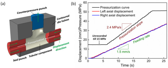
Figure 3.
(a) Schematic representations of the tube hydroforming processes. (b) Typical loading curves for tube hydroforming.
3. FEM Modelling of Tube Hydroforming
3.1. Modelling Method
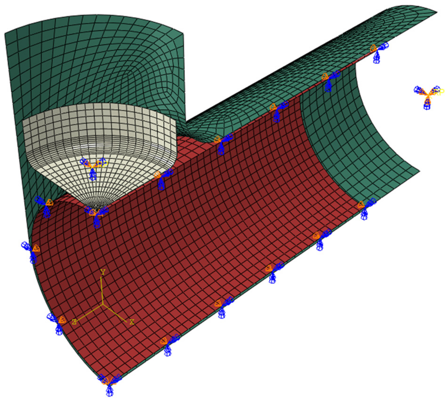
According to the FEM-ML technologies mentioned in the Introduction, an FEM model for tube hydroforming should be developed as the prerequisite for database generation. To this end, the Abaqus-explicit software (version 2022) was employed for FEM modelling. As shown in Figure 4, the geometrical model we applied is composed of two tool parts (counterpressure punch and contoured die) and the tubular blank, while the axial feeding of the seal punches is replaced by applying a prescribed displacement curve on the nodes at the tube edges. Taking the advantage of asymmetry, the geometry is simplified as one fourth of the problem. Meanwhile, benefiting from the large diameter-to-thickness ratio (~36) of the tube, the blank is discretized by 1360 elastoplastic shell elements with 1435 nodes, and the tools are regarded as analytical rigid bodies. Consequently, the total degrees of freedom of the model are reduced significantly and so are the computational expenses. It should be mentioned that all the shell elements have a dimension of 3.995 × 3.95 mm, namely, they are actually rectangular rather than square. Additionally, the friction coefficient between the tools and blank is set to 0.1, owing to the application of molybdenum disulfide powder [47].

Figure 4.
Simplified finite-element model of the hydroforming process.
3.2. Constitutive Modelling
For simulations of the tube hydroforming process, an appropriate constitutive model is crucial to correctly describe the material flow and avoid the unrealistic bursting of the tube. According to the study by Baral et al. [45] with respect to the plastic behavior of CP-Ti plates, among the commonly used models, the CPB06 yield criterion shows the best performance in capturing both the tension–compression asymmetry and the plastic anisotropy. In the light of that, the CPB06 model is applied to model the constitutive behavior of the titanium tube in the present work.
The mathematical expression of CPB06 model is written as follows [48]:
where a and k are material constants. Σ1, Σ2, and Σ3 are the three principal values of Σ (hereinafter the bold character denotes tensors or matrixes), which is a second-order tensor after linear transformation on the stress deviator S:
where C is a fourth-order symmetrical tensor involving nine independent components:
In the case of the thin sheet (plane stress) problem, there would be C44 = C55 = 0 and only three non-zero stress components (σx, σy, τxy) in the stress tensor. Then, the four non-zero components in Σ can be readily deduced:
and hence, the principal values are as follows:
Furthermore, in the CPB06 framework, the effective stress equivalent to that of the uniaxial tension along RD is as follows:
where
As we pointed out in Section 2, the present material exhibits a quite similar plasticity anisotropy with that observed by Baral et al. Hence, here we utilize the anisotropic parameters (C11~C66, a, k) proposed by them [45], which evolve with the cumulation of plastic work, except parameter a (a = 2). Now, the question is to model the hardening behavior of the material under uniaxial tension. Following the recommendation by [43,44], a modified K-T hardening law is employed for pure titanium:
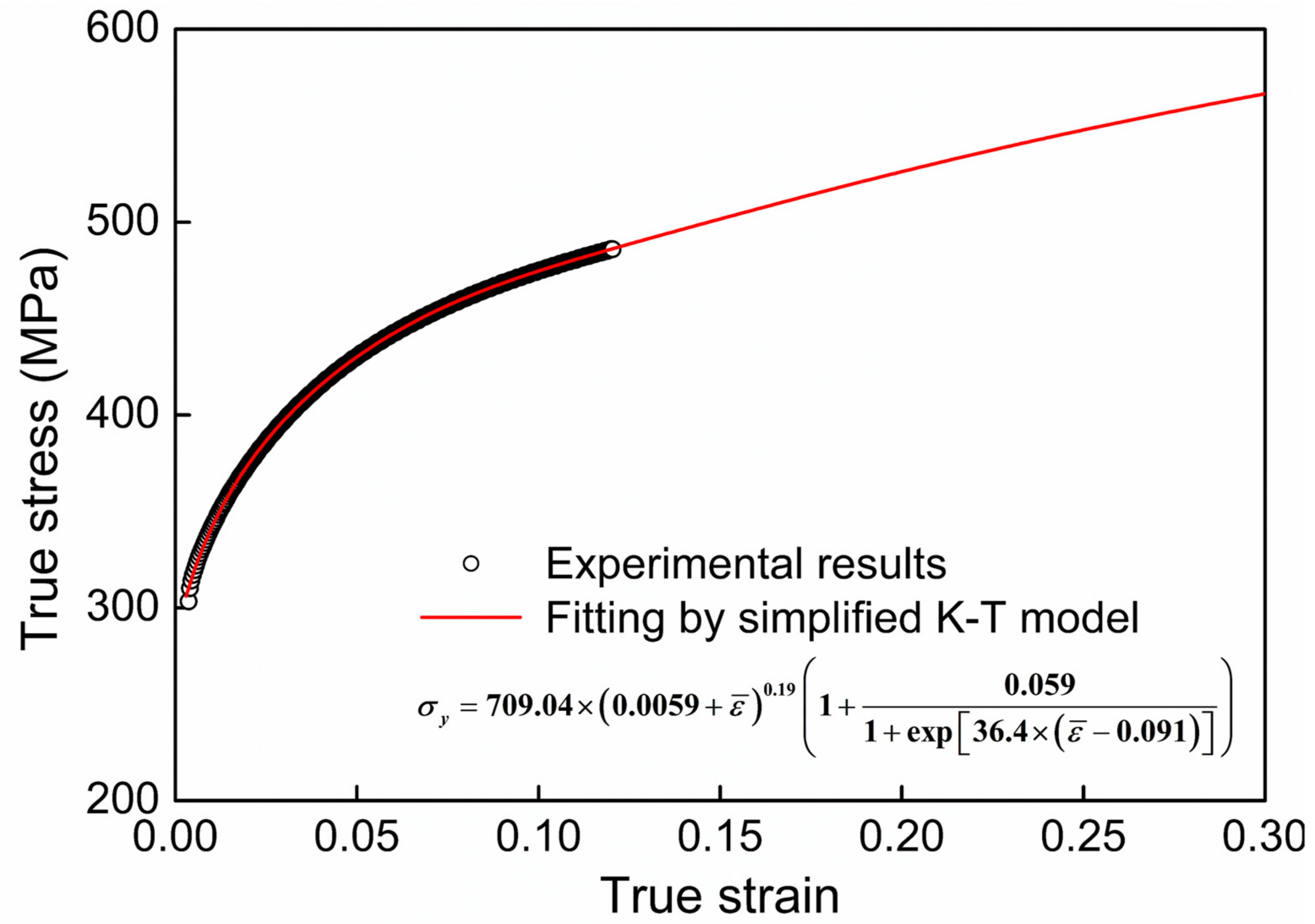
where S, K, ε0, h, a, t, and εs are the material parameters, σy and are the effective stress and plastic strain, respectively. Because only the small section of the hardening curve prior to the UTS point is available for fitting, we further simplify the hardening law by ignoring parameter S in Equation (8). As demonstrated in Figure 5, the simplified K-T model reproduces the existing hardening curve perfectly, while it is questionable for the extrapolated part beyond the UTS point. Nevertheless, the feasibility of the extrapolation can be examined by comparing the simulated results with the experiments, as shown later. Moreover, the emphasis in the present work is placed on the methodology of FEM-ML for real-time hydroforming simulation, rather than pursuing the precise accuracy of the FEM model.

Figure 5.
True stress–true strain curve (symbol) obtained by uniaxial tension in RD and the fitting/extrapolation results (solid line) by the simplified K-T model.
3.3. Numerical Implementation and Verification
In order to implement the developed CPB06 yield criteria in the FEM model, an explicit integration algorithm is applied to update the stress and plastic strain tensors, in which the plastic multiplier dλ is derived explicitly as follows [11]:
where f is the yield function, σ is the stress tensor, and Ce is the elastic stiffness matrix. To make the computation more stable, the flow tensor, ∂f/∂σ, takes the average value in the current and the previous increment. Then, the plastic strain and stress increment (Δσ) can be derived from the flow rule:
where Δε and Δεp denote the total strain increment and plastic strain increment in the current incremental step. In comparison with the commonly used semi-explicit integration algorithm in which the plastic multiplier is calculated implicitly via the Newton–Raphson iteration scheme, the proposed explicit integration is found to be more robust and significantly timesaving, while the computational accuracy is comparable to the former due to the small increment size. The CPB06 yield criterion (Equation (6)), together with the hardening model (Equation (8)), were embedded into Abaqus through the UMAT subroutine interface, under the framework of the associated flow (Equations (9) and (10)).
The simulation of uniaxial tensile tests following the experimental procedure is carried out to verify the constitutive model. As demonstrated in Figure 6a, the model accurately captures the mechanical response, especially the post-necking behavior. Moreover, the strain ratio of the axial (εy) to transverse direction (εx) is extracted from the critical point located in the specimen center and compared to the experimental results measured with DIC, as shown in Figure 6b. The acceptable consistency indicates the availability of the proposed constitutive model.
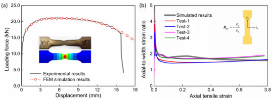
Figure 6.
(a) Comparison between the simulated results (symbol) and the experimental results (solid line). (b) Evolution of the axial-to-width strain ratio of the tensile specimen using FEM simulation (bold lines) and tensile tests (thin lines).
In addition to the uniaxial tension, various tube hydroforming processes are also simulated to evaluate the FEM model by applying the forming parameters tabulated in Table 2. As shown in Figure 7a, the total height of the tube branch is accurately predicted with remarkably small errors of only 1.0~1.6%. The good agreement indicates that the developed FEM model can be utilized in a wide range of processing conditions. Meanwhile, the von Mises yield criterion is also examined for comparison. As observed in Figure 7a, it predicts a much larger branch height for sample 1, with a deviation of ~14%. Meanwhile, the other two samples are even bursting under the von Mises criterion, which is totally inconsistent with the experiments. This, however, is anticipated, since the von Mises criterion ignores the distortional hardening effect such that the material becomes much too soft.

Table 2.
Processing parameters applied to verify the FEM model.
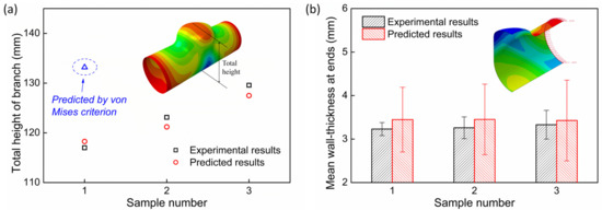
Figure 7.
Comparison of the (a) total branch heights and (b) wall thicknesses of the tube ends between the prediction and the measured results.
In addition, the wall thickness at the ends of the tube is compared for the experiment and the prediction in Figure 7b. Note that for all the conditions, the thickness is slightly overestimated by a factor of 3~7%. This may be partially caused by the ignorance of the seal punches during modelling, which results in the “free” thickening of the tube edges. Nevertheless, the small deviations further confirm the reasonability of the developed hydroforming FEM model.
4. FEM-ML Model Formulation
4.1. Conceptional and Methodological Basis
The FEM simulation tests manifest that when the axial feeding rate is 1.5 mm/s, the CPU time required for one simulation run reaches 7320 s, even if a relatively large incremental time step (5 × 10⁻⁵ s per increment) is used. In marked contrast, the actual forming time is only about 23 s. As pointed out in the Introduction, such a large difference is intrinsically attributed to the numerical algorithmic nature of the FEM. In an elastoplastic problem, the computational workflow of the FEM can be simply concluded as follows if the implicit algorithms are applied [10]: (1) assuming the displacement field via shape functions → (2) calculating strain via kinematical equations → (3) deriving stress via constitutive equations (simultaneously extracting plastic strain) → (4) computing displacement and related variables via equilibrium equations. Apparently, the computational loop is rather time-consuming due to the complicated iteration and matrix/tensor operations. Although the step 4 can be avoided under the explicit algorithms, the time increment must be set to be very small to avoid the computational instability [11].
Indeed, the displacement field (more exactly the velocity field) is the primary unknown quantity that is required to be solved in a mechanical problem. Assuming that the displacement field is already known, one can readily deduce other physical fields in a subsequential manner. The specific methodology is described below.
Figure 8a shows a shell element with a prior rectangular shape, and it is subject to an arbitrary in-plane deformation from configuration (a) to (b). Supposing that the nodal coordinates (A, B, C, D) before and after the deformation are established, the strain is therefore able to be deduced by various methods. From the perspective of simplification, here we applied the approach proposed by [49], in which the principal strains are derived from the Cauchy–Green deformation tensor. Owing to the simple rectangular shape of the initial element, the two in-plane principal strains (i.e., ε1 and ε2) can be obtained through a simple algebraic calculation. Sequentially, the out-plane principal strain (ε3) can be furnished by the incompressibility assumption, as well as the shell thickness, t:
where t0 represents the shell thickness prior to deformation. The effective (equivalent) strain is therefore given by the following:
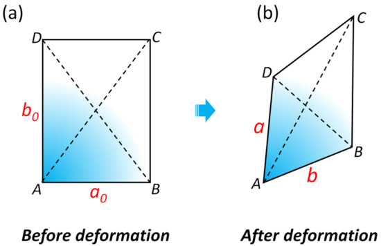
Figure 8.
(a) A shell element ABCD with a rectangular shape prior to deformation. (b) The shape of the element after arbitrary deformation. a0 and b0 denote the edge lengths prior to deformation while a and b are those after deformation.
Then, if the elastic deformation is ignored, the effective stress can be directly obtained by substituting the effective strain into the hardening model (Equation (8)).
According to the analysis above, the field variables during hydroforming are sequentially derived through simple algebraic calculations on nodal coordinates. Again, it should be stressed that the elastic deformation is ignored in the computational sequence to evade time-consuming iterative calculations, enabling the extraction of the plastic strain from the total strain. However, it has little effect on the accuracy of the field variables because the elastic deformation is negligible in such a hydroforming process. On the other hand, the displacement field has already been predefined according to our methodology, which can minimize the elastic effect on the deformation.
4.2. Development of the Framework
In Section 4.1, we have recognized that an instant acquisition of the displacement field, or more specifically the nodal coordinates, is the key step for the real-time simulation of tube hydroforming. Following the FEM-ML framework as introduced in Section 1, the offline FEM simulation can be utilized to generate various datasets for nodal coordinate evolution, while a surrogate model based on ML is developed for the instant prediction of the nodal coordinates. However, this is rather difficult for the present case since there are 1435 nodes even in the simplified FEM model (Figure 4) and their coordinates would continuously change with straining. Now, the primary issue we faced is how to design the input variables for ML as well as the collection of data samples for training. Two solution schemes may be available, as shown below.
4.2.1. Scheme 1
A simple fact is that the evolution history of the nodal coordinates would be changed with the loading conditions such as the axial feeding rate, target internal pressure, pressurization slope, etc. Therefore, in a rather straightforward manner, all the loading parameters can be utilized as the input variables for ML, while the output variables are regarded as all the nodal coordinates at every time increment during forming. Accordingly, the database for ML training is constructed through numerous FEM simulation runs using various loading parameters. After the training of the ML model, the developed surrogate model can infer the momentary coordinates of nodes according to the real-time processing parameters, and thereby the multi-physical fields. Such a straightforward strategy is expected to have a good performance in predicting the effect of loading fluctuation on hydroforming. However, it faces a fundamental problem. Assuming that the loading histories are fairly stable among all the processing cycles, the FEM-ML model would give identical feedback every time. In this circumstance, the model would be less meaningful since a virtual monitoring system like that should be more focused on abnormity than normality. Imaging in an extreme case that the tubular blank is trapped in the die cavity during hydroforming, the surrogate model would be incapable of reflecting the real deformation state since all the loading parameters it acquired remain routinely normal. The disconnection between prediction and reality renders scheme 1 to be inappropriate in the present study.
4.2.2. Scheme 2
The origin of the tube hydroforming defects is essentially attributed to the velocity mismatch between the inward material flow (into the die cavity) and that of the axial feeding. If the former is excessively faster, “thinning-type” defects would appear in the forms of excessive wall-thinning, necking, cracking, fracturing, bursting, etc. On the contrary, “thickening-type” defects would occur if the axial feeding is more pronounced, such as inadequate filling, over-thickening, buckling, wrinkling, folding-back, etc. All these defects, which are caused by an inappropriate material flow, would have a direct influence on the external volume of the tubular components and hence the free boundaries. In the present case, as shown in Figure 3a, the component is closely pressed against the die by the internal pressure and the position (displacement) of the tube ends is precisely controlled. Then, any quality drawbacks could be reflected by the relative bulging velocity of the tee-branch (i.e., the motion of the counterpressure punch), as it is the only free boundary. Accordingly, in this scheme we adopt the two boundary conditions as the input variables in the ML model, namely, the controlled motion of the tube ends and the passive displacement of the counterpressure punch. The output variables are still the nodal coordinates. In contrast to scheme 1, this scheme seems more reasonable since it enables the capturing of an abnormal metal flow caused by unexpected factors.
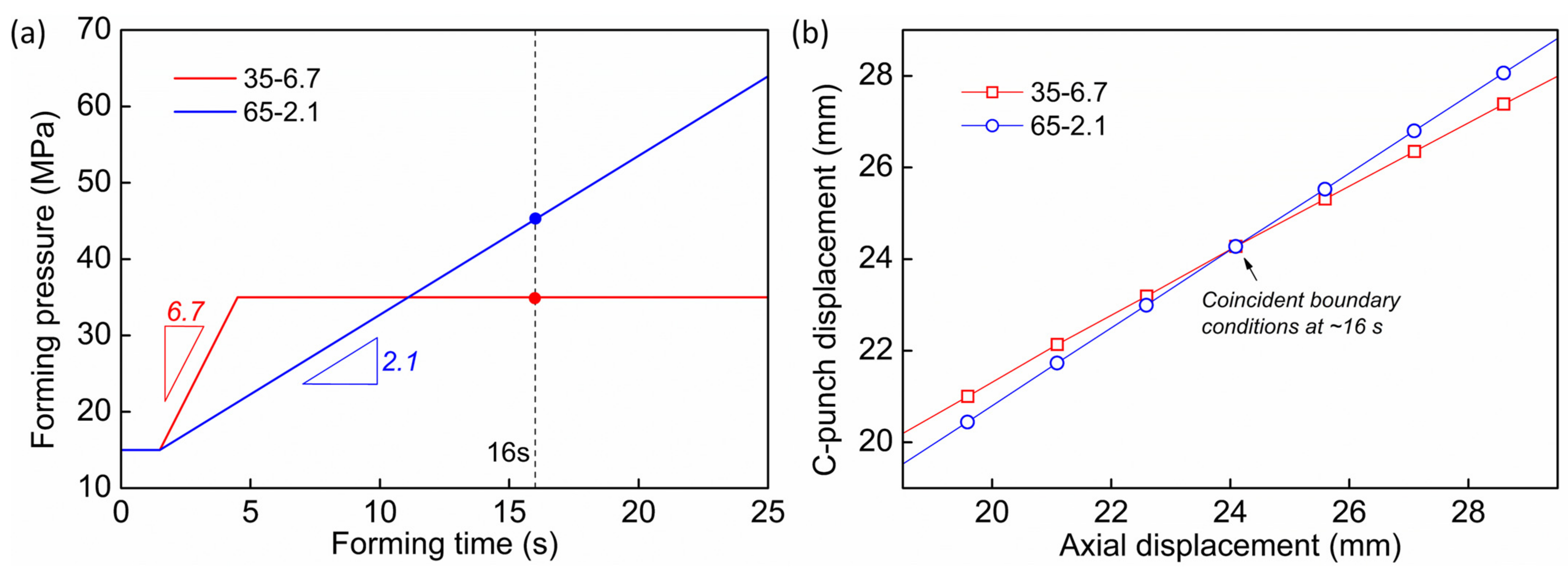
However, scheme 2 also faces the primary concern that it may be not a one-to-one mapping relation between the displacement field and the boundary condition. That is, there may be more than one displacement field corresponding to a certain boundary condition, so that it would be misleading when inferring the former from the latter by ML models. To examine this point, a series of FEM simulations have been performed by employing different pressurization paths as typically described in Figure 9a, whereas the axial feeding rates are identical (1.5 mm/s). Thereinto, the sample label, 35-6.7 or 65-2.1, means that the target pressure is 35 MPa (65 MPa) with a pressurization slope of 6.7 MPa/s (2.1 MPa/s). The obtained displacement boundaries of the two simulation runs are shown in Figure 9b, where the vertical axis denotes the passive displacement of the counterpressure punch, and the horizontal axis represents the axial feeding distance. Note that there exists an intersection point on the displacement curves, indicating that the boundary conditions are transiently coincident despite the fact that the loading paths are far from identical. As indicated in Figure 9a, the corresponding internal pressures at that point (~16 s) are 35 MPa and 45.4 MPa, respectively.
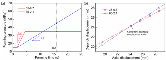
Figure 9.
(a) The pressurization curves of the two hydroforming simulation runs. (b) Predicted displacement curves of the boundaries for the two virtual tests.
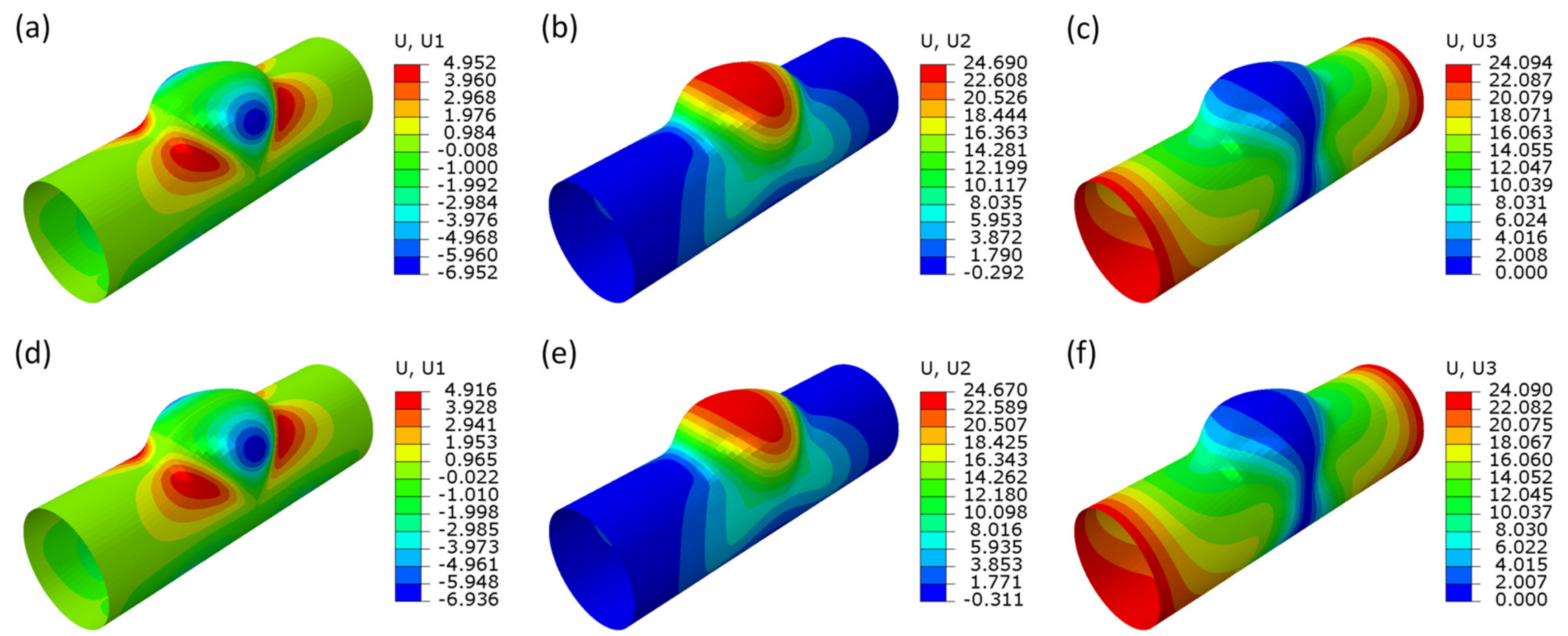
Figure 10 shows the displacement fields of the two samples at the time point when the boundary conditions are coincident. One can note that the displacement field is nearly identical both in terms of distribution and gradient. The maximum deviation is only less than 1%. In a word, the deformation state of the tubular component at a certain time point can be well reflected by the concurrent boundary conditions. It should be mentioned that this observation is not a coincidence but has been demonstrated as a common phenomenon in the present case. Therefore, the one-to-one collocation between the displacement boundary condition and the displacement field is confirmed, as well as the reasonability and availability of the scheme 2. Further discussion with respect to this point will be carried out later.
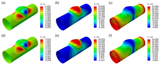
Figure 10.
Comparison of the displacement field between (a–c) sample 35-6.7 and (e,f) sample 65-2.1 under the same boundary condition shown in Figure 9. (a,d), (b,e), and (c,f) are displacement distributions in the x, y, and z direction.
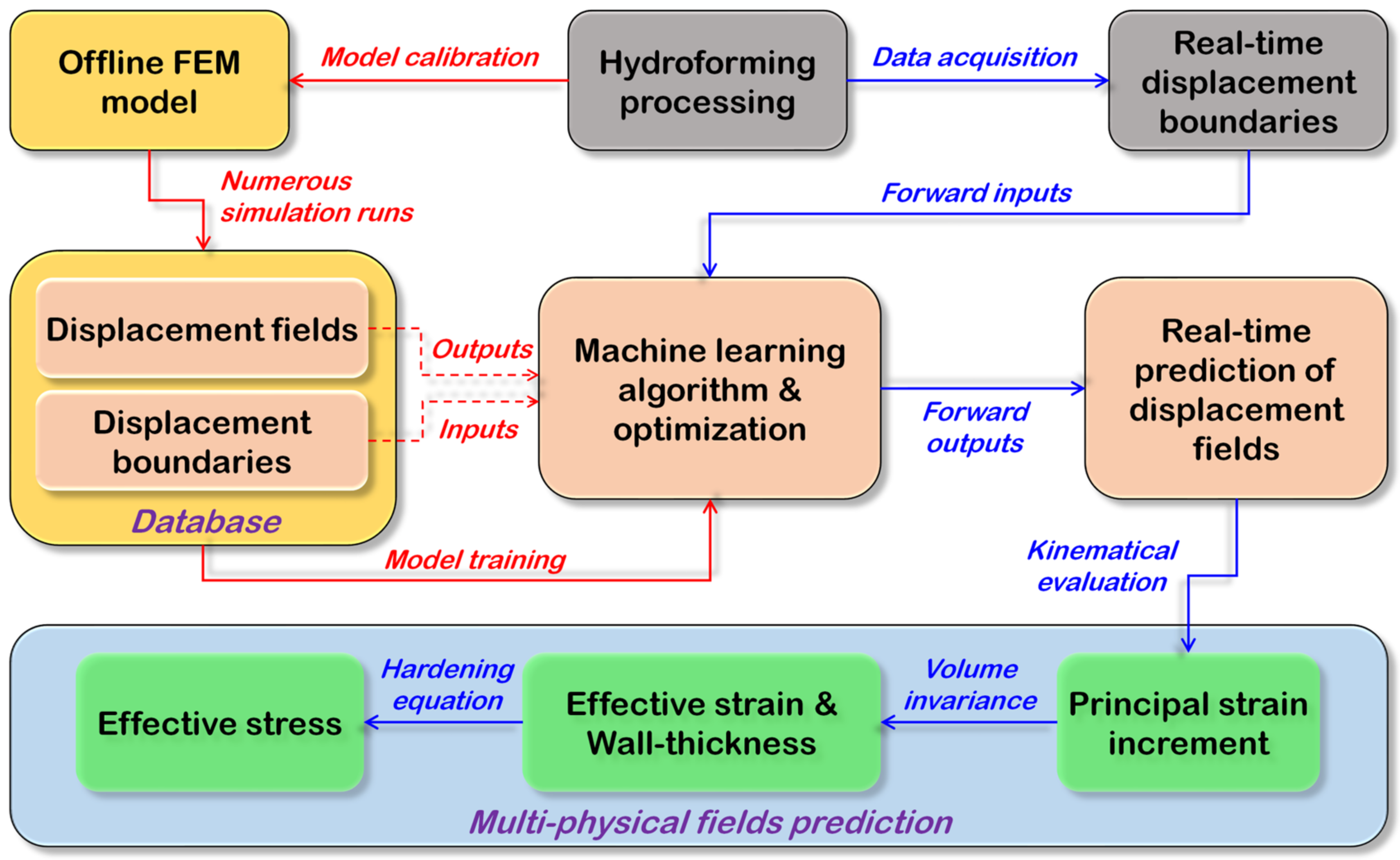
Based on the analysis above, the FEM-ML framework can be constructed for the present case. As schematically overviewed in Figure 11, the framework consists of three parts that are interrelated, i.e., the offline FEM, the physical part, and the ML-based surrogate model. Based on the hydroforming process, the offline FEM is calibrated and applied to generate the training database, which is accomplished by full-field simulations under various loading paths. Time series data with respect to the displacement boundaries and the displacement fields are extracted from the simulation output files. To balance the precision and the efficiency, the time interval for data collection is set to be 0.5 s during the entire forming process. Then, the database is used to train the ML model, in which the input data are the displacement boundary conditions, and the displacement fields are treated as output. After that, the real-time displacements of the counterpressure punch and the seal punch are acquired by the well-trained surrogate model. Once the input dataset is received, the surrogate model will instantly predict and visualize the coordinates of all nodes to show the current shape of the tube component. Meanwhile, the coordinate values are used to calculate the total principal strain by comparing them with those in the undeformed state. Thereby, the concurrent equivalent strain, the current wall-thickness, and the effective stress are derived simultaneously and contour-plotted on the pseudo-integration points.
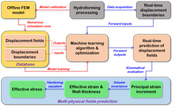
Figure 11.
Structure and workflow of the proposed surrogate model.
4.3. ML Method and Training Strategy
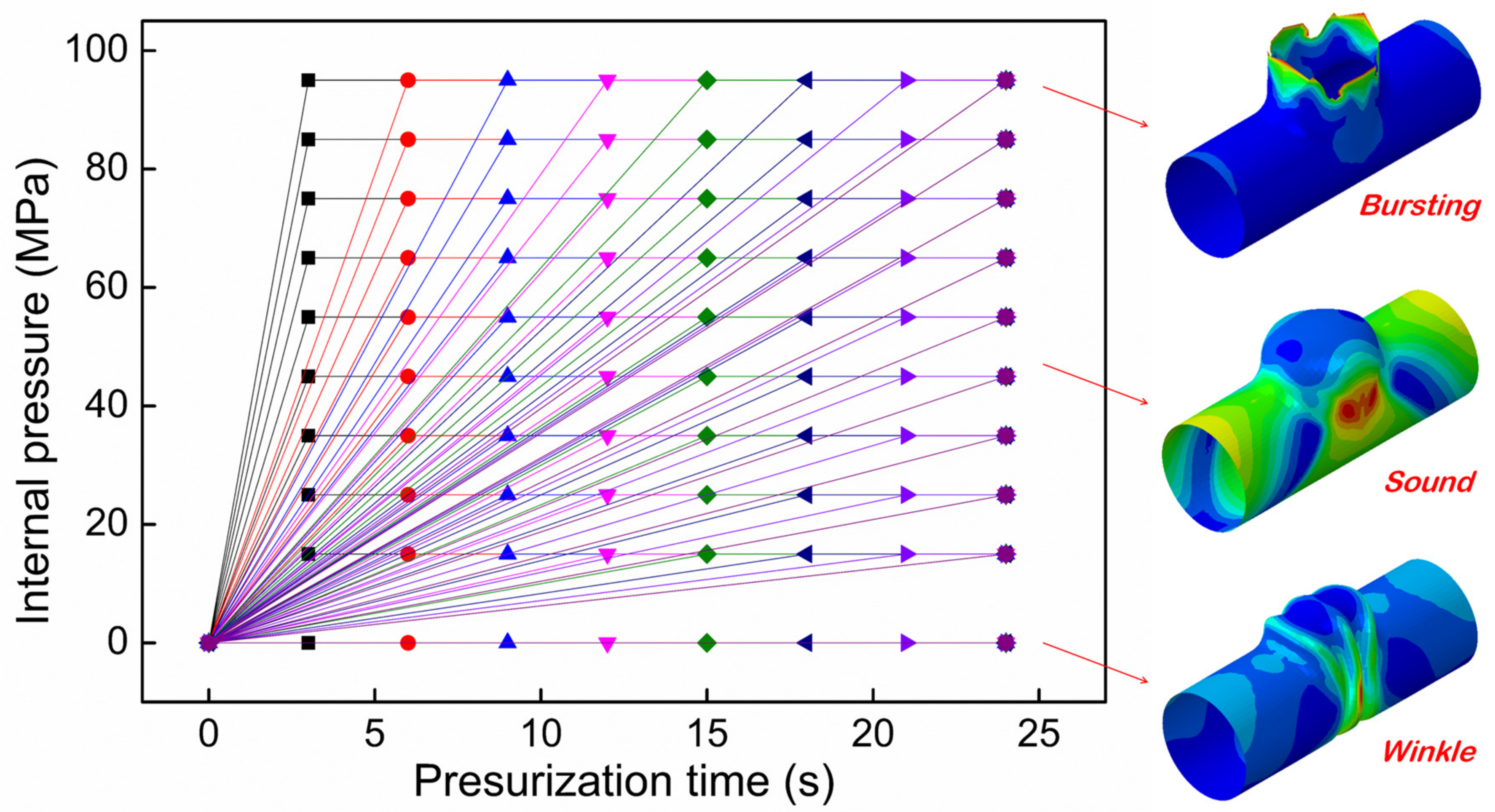
A well-organized database is the basis for the efficient training of the ML model. As emphasized earlier, the deformation state of the tubular component is up to the relative displacement/velocity of the counterpressure punch and the seal punch. Hence, a fixed feeding rate of 1.5 mm/s is utilized for the seal punch in all the simulation runs, while the pressurization curve is changed in a wide range to introduce differences in the free boundary. For that, a parameter grid is created, as seen in Figure 12, which roughly covers the capability of the hydraulic forming facility and various forming defects from wrinkling to bursting. The produced database consists of the two displacement boundaries, the nodal number, and the three coordinate values for each node. Because of the occurrence of bursting under ultrahigh internal pressure, some of the time series data are incomplete. The obtained database for ML training has more than 2.4 million lines of data generated from 73 FEM simulation runs.
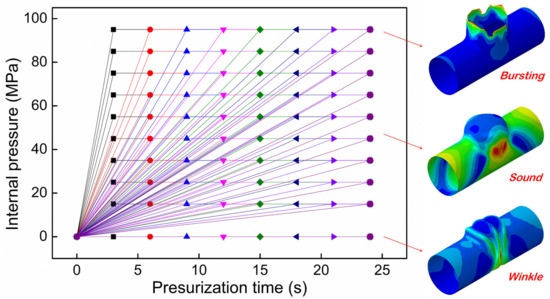
Figure 12.
The parameter grid showing various pressurization curves used for simulation. The insert graphs depict forming defects at different forming conditions.
The question now is to select the proper ML algorithm. Among the commonly used algorithms in structural engineering such as Bayes classifiers, linear and logistic regression, decision trees/random forests, support vector machines, artificial neural networks/deep learning, etc. [38,50], the random forest algorithm (RFA) is a very popular algorithm in both regression and classification problems and can efficiently capture the nonlinearity in data [51]. The RFA is an ensemble method built on a number of weak decision trees to obtain a more stable and accurate prediction. Each tree is built on a random subset of the training data; thus, this method can bring stochasticity while training the model, which helps in avoiding overfitting issues. The RFA can handle both numerical and categorical features and deal with missing or unbalanced data efficiently [36]. Therefore, the RFA has been demonstrated to be a very robust regressor and classifier with good accuracy even for abnormal and noisy data [52]. In addition, the training and inference calculations are very easy and fast for the RFA. To date, the RFA has achieved great success in FEM-ML frameworks [18,20,36]. Given the fact that the data samples are quite limited in contrast to the large data volume, the RFA is applied in this work to avoid overtraining and overfitting.
The RFA framework was developed in Phcharm by calling the sklearn toolkit. For an ML algorithm, hyperparameter tuning is the critical step. In the RFA, there are primarily five required parameters to be considered: the number of trees (ntree), the maximum depth of the tree (dmax), the number of features (nfeature), the minimum number of samples on a tree node (nnode), and the minimum number of samples on a tree leaf (nleaf). In order to achieve good performance on the training data as well as generalize well on unseen data, 70% of the data are randomly selected from the whole database and used for training, while the rest are for validation. Then, the optimal hyperparameter combination is determined through the grid search method. The grid search method tests each set of possible combinations of the parameters and the one with the highest accuracy is selected as the optimal value. The search space for all hyperparameters is tabulated in Table 3, which results in a total of 960 possible combinations. In addition, the MAE (mean absolute error) and R2 (adjusted R-square) are selected as the measures of the predictive accuracy performance, which are, respectively, defined as follows:
and
where yi, , and are the values produced using the FEM, the predicted values using the ML model, and the predicted mean values using ML model, respectively. N is the total number of the data lines in the database.

Table 3.
Search space for hyperparameter tuning of ML models and the optimal parameter combination.
4.4. Validation of the Model
The optimal combination of hyperparameters after the parametric tuning of the RFA are tubulated in Table 3. For both training and testing datasets, a high prediction capability was achieved with an MAE less than 0.02 and R2 higher than 0.999, even though the testing datasets are not used for training. This manifests that the developed surrogate model appears to have a high generalization capability. Meanwhile, the response time of the model is less than 0.004 s once the input data are passed through, which is negligible in comparison with that of the offline FEM simulations.
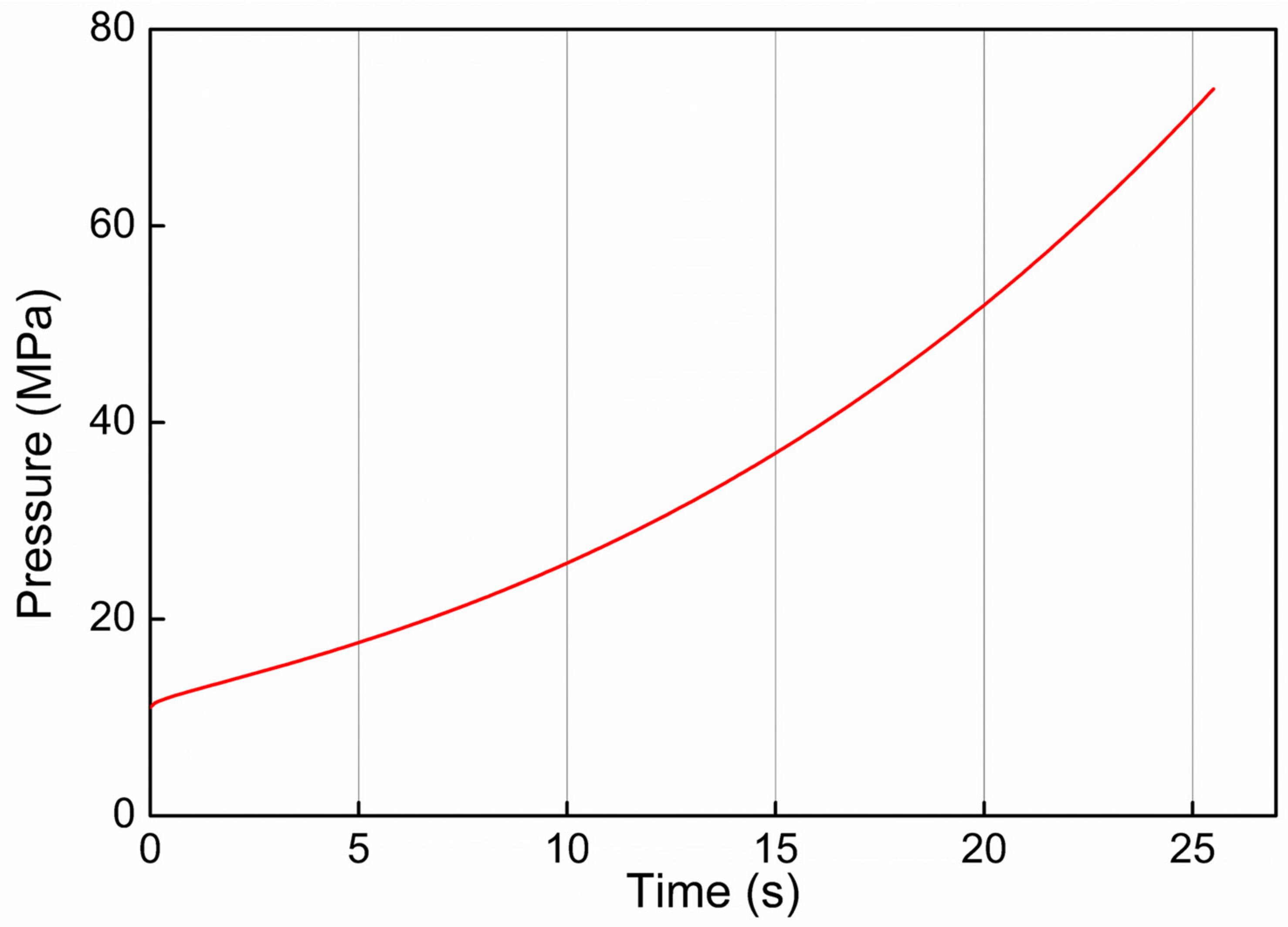
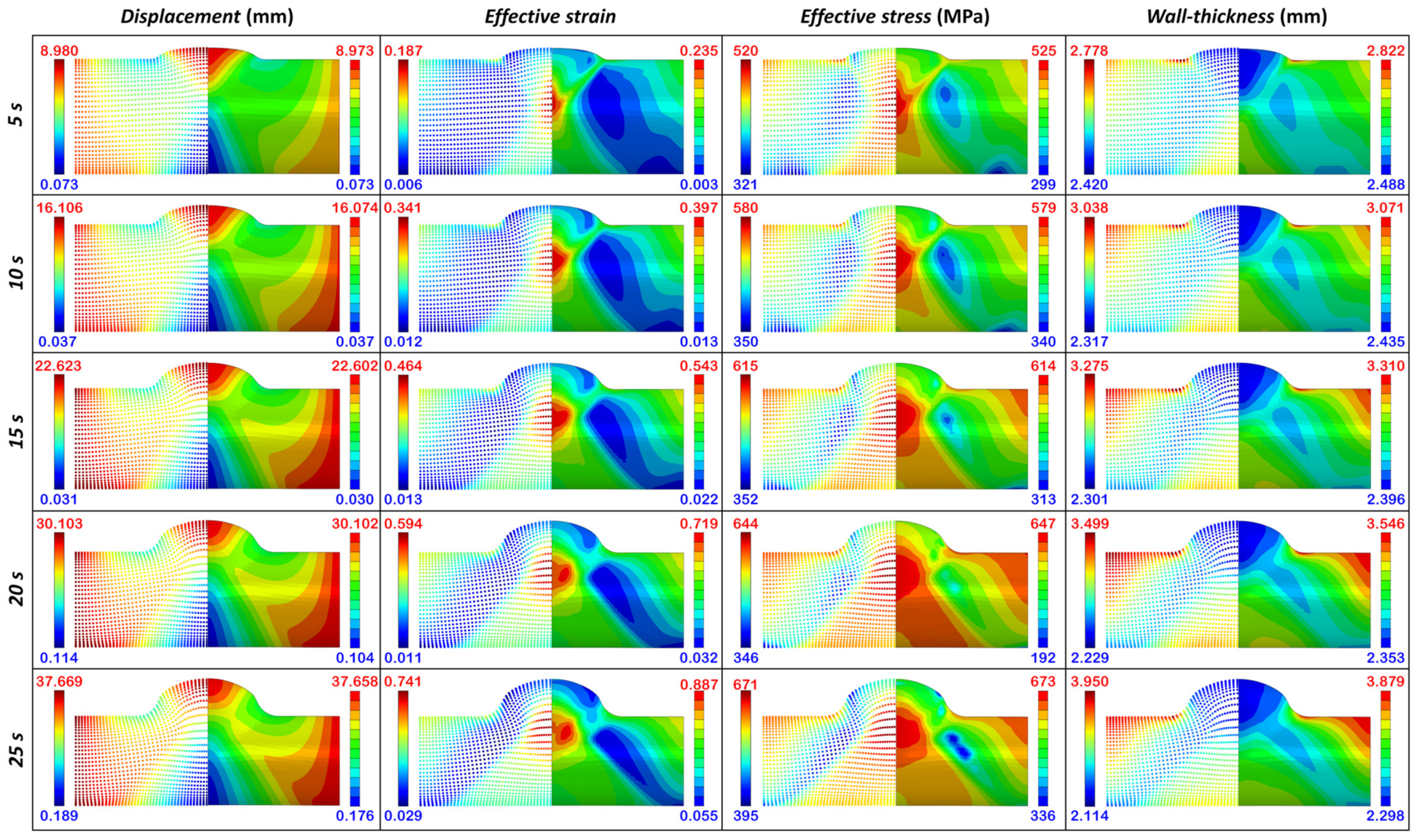
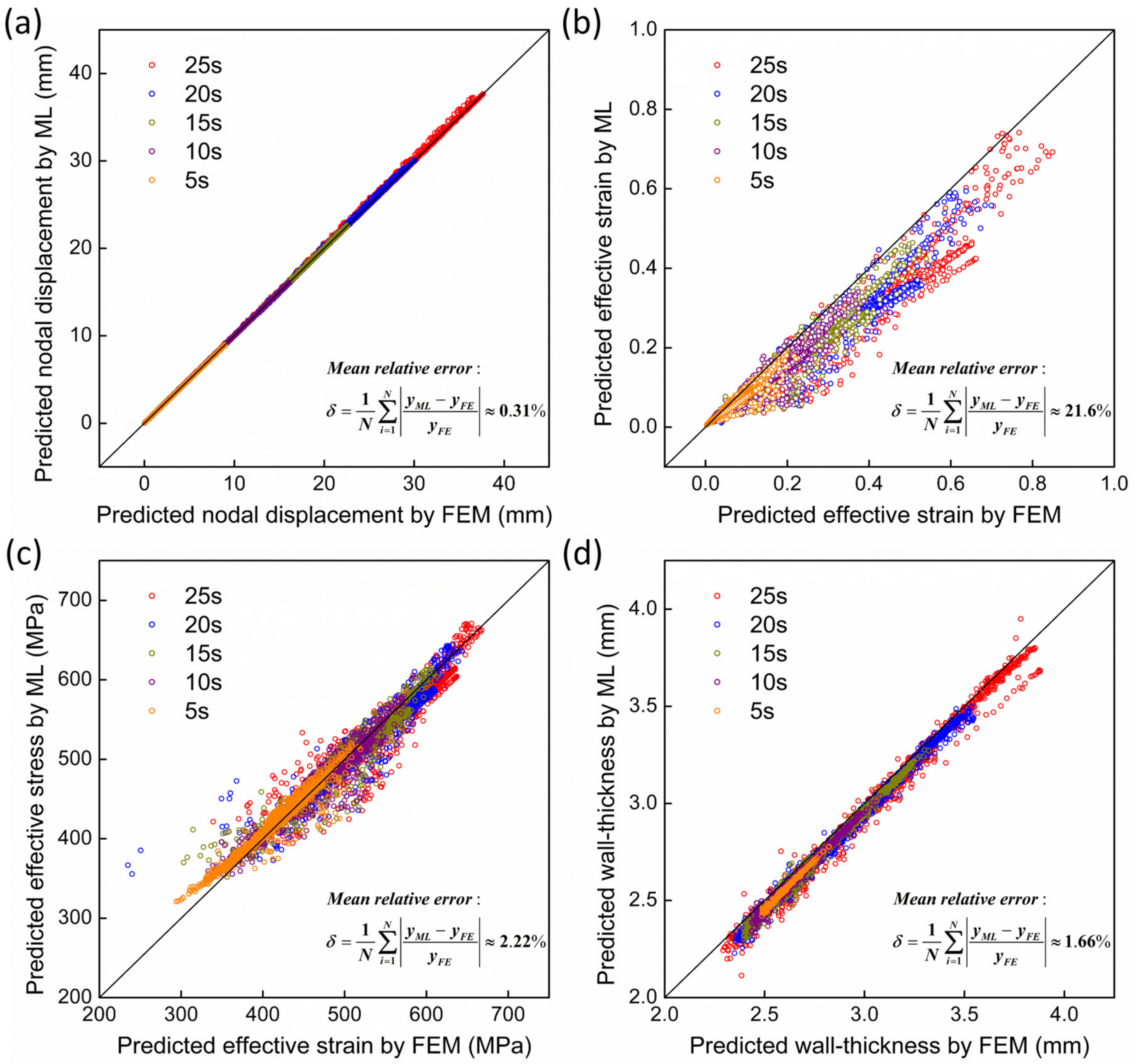
The reliably and the extrapolation ability of the surrogate model is verified using the third testing dataset, which is produced by a new FEM simulation run for hydroforming. In particular, the pressurization curve is set in such a way that it increases exponentially toward the target value (refer to Figure 13), while the axial feeding rate keeps a constant 1.5 mm/s. Apparently, this loading condition has not been taken into account by the training dataset and is also impossible in real industrial applications. Figure 14 shows the multi-physical fields predicted by the surrogate model along with those calculated by the offline FEM at various forming stages. At a first glance, one can notice that the distribution and evolution features of all the field variables are accurately predicted by the surrogate model. Specifically, it yields almost identical displacement fields with the FEM model. A quantitative comparison of the absolute displacement for all nodes is shown in Figure 15a. The small mean error (~0.31%) confirms a perfect agreement between the surrogate model and the FEM simulation. Despite the high accuracy, one may speculate that the present ML model has not been overtrained/overfitted since the distribution of the displacement fields is quite smooth (Figure 14). Otherwise, a zigzag tube appearance or striped contours would be presented. Therefore, one can conclude that the developed model enables the reliable prediction and real-time monitoring of the deformation states during tube hydroforming.

Figure 13.
Pressurization curve used for the extra-simulation test.
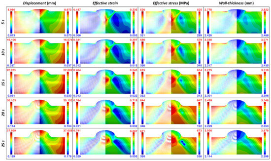
Figure 14.
Comparison of multi-physical field between those predicted by surrogate model (dot) and the FEM model (solid) at different forming times. The loading condition is depicted in Figure 13.

Figure 15.
Quantitative comparison of the predicted field variables between ML model and offline FEM model for all nodes/elements at various forming times: (a) displacement of nodes; (b) effective strain of elements; (c) effective stress of elements; (d) wall thickness. The mean error is also tabulated in the figure, where yML and yFE are the predicted results by ML model and FEM model, respectively.
The situation is changed for the effective strain field. As shown in Figure 14 and Figure 15b, in most elements, the effective strains are notably underestimated by the surrogate model with a mean error of ~21.6%, even though the elastic strain is included. In fact, we have made systematic studies in terms of one-element-testing and found that the proposed computing sequence deriving the strain from the displacement field is quite reliable. Then, two factors may account for the relatively large deviation in strain prediction. Firstly, despite the precisely accurate displacement field that is predicted by the surrogate model, the strain at a certain point depends on the relative displacement of the adjacent nodes rather than the absolute displacement. Trivial displacement errors would be magnified and reflected by the derived strain values with consideration for the small element size. Meanwhile, the well-trained ML model intrinsically predicts a smoother displacement field (than that by FEM simulation), which inevitably leads to the underestimation of the local strains. Secondly, when estimating the effective strain in an element, the deformation is thought to be homogeneous within the element. However, in the FEM model, there are two integration points within the applied element type. The over-homogenization would further decrease the strain maxima.
Since the effective stress field is derived from the hardening equation (Equation (8)) by using the effective strain, it is not surprising that the stress values are frequently underestimated, as shown in Figure 15c. Nonetheless, the prediction accuracy with a mean error of 2.22% is much better than that for effective strain, indicating that the stress is rather insensitive to the strain fluctuation.
An interesting phenomenon is noticed with respect to the wall thickness. As shown in Figure 14 and Figure 15d, the wall thickness is only slightly underestimated with a mean error of 1.6%, which is in stark contrast to the effective strain. Also, the highly aligned datapoints in Figure 15d indicate that the out-plane principal strain, i.e., ε3 in Equation (11), can be perfectly predicted by the model. Since ε3 is derived from the incompressibility assumption, one may surprisingly notice that the prediction errors of the two in-plane strain components are subtly compensated by each other, probably owing to the smoothing and homogeneity of the displacement field.
5. Discussion
In this work, we tried to develop a surrogate model for the real-time, full-field simulation of the tube hydroforming process by integrating the FEM and ML algorithm. The proposed modelling methodology, which mainly involves the reverse derivation of the displacement fields from the given boundary conditions, demonstrates its accuracy and instantaneity in predicting multi-physical fields, especially the displacement field and wall-thickness evolution. Meanwhile, the proposed framework is expected to be advisory and informative to other plastic forming processes. Although success has been seemingly achieved in this exploratory attempt, some limitations exist within the model and further improvements are required.
In an FEM-ML framework, the FEM plays a fundamental role because it acts as a database generator. Its accuracy basically determines the validity of the training data. With regards to the tube hydroforming process, an accurate constitutive model, which can describe the yield surface evolution with a wide range of straining, is primarily crucial for plastic anisotropic metals such as titanium. However, the experimental determination of the yield surface is rather difficult at a relatively high strain. The frequent utilization of extrapolation and approximation inevitably affects the predictive accuracy. This point has been clearly manifested in Section 2. Furthermore, the strain rate sensitivity is ignored in the present study, which may also affect the results to some extent. In addition, an appropriate failure model capable of predicting multiaxial damage behavior should also be incorporated to achieve a better performance of the FEM model.
On the other hand, the major concern of the developed model is to provide a real representation of the (abnormal) deformation state of the tube component. To meet this objective, the reverse inference methodology we proposed is based on the acquisition of two displacement boundaries. Although it is fairly reasonable according to our analysis (Section 4), the methodology is still idealized, since it ignores many processing fluctuations both in forming conditions (e.g., the lubrication instability) and blank materials (e.g., inhomogeneous distribution of thickness and mechanical properties). This may cause an incorrect displacement field when it is inferred from the boundary conditions. However, these fluctuations are unpredictable and hardly quantified, such that it seems unable to be considered by the FEM-ML model. Experimental efforts are required to confirm the effects of these fluctuations on the hydroforming qualities. Nevertheless, since the rise in any hydroforming defects can somehow be reflected by the boundary conditions (analyzed in Section 4.1), the developed surrogate model is at least able to act as a predictor of forming defects, even if the displacement field cannot be inferred correctly in unforeseen circumstances. Anyway, the surrogate model will be packaged as software and embedded into the hydroforming machine. Systematic testing will be conducted to optimize and upgrade the model.
6. Conclusions
In this study, an FEM-ML framework was developed to facilitate the real-time, full-field simulation of the hydroforming process for titanium tubes, whereby the multiple physical fields can be predicted synchronously with the actual processing. To this end, we proposed a methodological foundation in which the computational workflow of the FEM was interrupted and reassembled using an ML-based surrogate model. The main conclusions are drawn below.
- (1)
- The titanium tube was characterized by a fine and equiaxed grain structure as well as a typical rolling texture. The CPB06 constitutive model, together with a simplified KT hardening model, were applied to capture the distinctive yielding behavior of titanium during multiaxial loading. Accordingly, an FEM model for the hydroforming process was developed, which can accurately predict the evolution of the multi-physical fields.
- (2)
- Based on the fact that there was a one-to-one collocation between the boundary conditions and the instantaneous displacement field during hydroforming, numerous FEM simulations were performed with various loading conditions to generate a database for ML training. The database consisted of the two displacement boundaries, the time series coordinates of all nodes, as well as their number. All the other field variables were derived from the variation of the coordinates, including the principal strain, effective strain, wall thickness, effective stress, etc.
- (3)
- A random forest algorithm was utilized to map the collocation from the displacement boundaries to the concurrent displacement field. To achieve better performance, the involved hyperparameters were tuned and optimized using the grid search method. For both the training dataset and testing dataset, the well-trained model exhibited a good performance with an MAE less than 0.02 and R2 value up to 0.999. In addition to the accuracy, the response time of the model was less than 0.004 s.
- (4)
- The developed model enabled the real-time, full-field simulation of the hydroforming process and the instant prediction of forming states. Specifically, while the effective strain was notably underestimated, the model showed outstanding accuracy and instantaneity in predicting the displacement field, effective stress, and wall thickness.
Author Contributions
L.C.: conceptualization, methodology, investigation, formal analysis, writing—original draft, and funding acquisition. H.G.: data curation, investigation, software, and visualization. L.S.: resources. C.Y.: software and resources. F.S.: resources and funding acquisition. J.L.: resources and writing—review and editing. All authors have read and agreed to the published version of the manuscript.
Funding
This work was funded by the National Science Foundation of China, grant number 51905233, and the National Basic Scientific Research Project, grant number JCKY2020607B003.
Data Availability Statement
Data will be made available on request.
Conflicts of Interest
Author Chao Yang was employed by Western Superconducting Technologies Co. The authors declare that they have no known competing financial interests or personal relationships that could have appeared to influence the work reported in this paper.
References
- Alaswad, A.; Benyounis, K.Y.; Olabi, A.G. Tube hydroforming process: A reference guide. Mater. Des. 2012, 33, 328–339. [Google Scholar] [CrossRef]
- Hartl, C. Mechanics of hydroforming. In Mechanics of Materials in Modern Manufacturing Methods and Processing Techniques; Silberschmidt, V.V., Ed.; Elsevier: Amsterdam, The Netherlands, 2020; pp. 71–109. [Google Scholar]
- Reddy, P.V.; Reddy, B.V.; Ramulu, P.J. Evolution of hydroforming technologies and its applications—A review. J. Adv. Manuf. Syst. 2020, 19, 737–780. [Google Scholar] [CrossRef]
- Johnson, K.I.; Nguyen, B.N.; Davies, R.W.; Grant, G.J.; Khaleel, M.A. A numerical process control method for circular-tube hydroforming prediction. Int. J. Plast. 2004, 20, 1111–1137. [Google Scholar] [CrossRef]
- Bell, C.; Corney, J.; Zuelli, N.; Savings, D. A state of the art review of hydroforming technology. Int. J. Mater. Form. 2020, 13, 789–828. [Google Scholar] [CrossRef]
- He, Z.B.; Zhang, K.; Zhu, H.H.; Lin, Y.L.; Fu, M.W.; Yuan, S.J. An anisotropic constitutive model for forming of aluminum tubes under both biaxial tension and pure shear stress states. Int. J. Plast. 2022, 152, 103259. [Google Scholar] [CrossRef]
- Tiji, S.A.N.; Park, T.; Asgharzadeh, A.; Kim, H.; Athale, M.; Kim, J.H.; Pourboghrat, F. Characterization of yield stress surface and strain-rate potential for tubular materials using multiaxial tube expansion test method. Int. J. Plast. 2020, 133, 102838. [Google Scholar] [CrossRef]
- Ortjohann, L.; Becker, M.; Niemietz, P.; Bergs, T. Monitoring of fluctuating material properties for optimizing sheet-metal forming processes: A systematic literature review. Mater. Res. Proc. 2023, 28, 2071–2080. [Google Scholar]
- Pham, Q.T.; Le, H.S.; Nguyen, A.T.; Xiao, X.; Kim, Y.S.; Nguyen, V.D.; Tran, H.S.; Tran, X.V. A machine learning–based methodology for identification of the plastic flow in aluminum sheets during incremental sheet forming processes. Int. J. Adv. Manuf. Techol. 2022, 120, 3559–3584. [Google Scholar] [CrossRef]
- Reddy, J.N. Introduction to the Finite Element Method; McGraw-Hill Education: New York, NY, USA, 2019. [Google Scholar]
- Dunne, F.; Petrinic, N. Introduction to Computational Plasticity; OUP Oxford: Oxford, UK, 2005. [Google Scholar]
- Butler, K.T.; Davies, D.W.; Cartwright, H.; Isayev, O.; Walsh, A. Machine learning for molecular and materials science. Nature 2018, 559, 547–555. [Google Scholar] [CrossRef]
- Morgan, D.; Jacobs, R. Opportunities and challenges for machine learning in materials science. Annu. Rev. Mater. Res. 2020, 50, 71–103. [Google Scholar] [CrossRef]
- Brodnik, N.R.; Muir, C.; Tulshibagwale, N.; Rossin, J.; Echlin, M.P.; Hamel, C.M.; Kramer, S.L.B.; Pollock, T.M.; Kiser, J.D.; Smith, C.; et al. Perspective: Machine learning in experimental solid mechanics. J. Mech. Phys. Solids 2023, 173, 105231. [Google Scholar] [CrossRef]
- Settgast, C.; Hütter, G.; Kuna, M.; Abendroth, M. A hybrid approach to simulate the homogenized irreversible elastic–plastic deformations and damage of foams by neural networks. Int. J. Plast. 2020, 126, 102624. [Google Scholar] [CrossRef]
- Nascimento, A.; Roongta, S.; Diehl, M.; Beyerlein, I.J. A machine learning model to predict yield surfaces from crystal plasticity simulations. Int. J. Plast. 2023, 161, 103507. [Google Scholar] [CrossRef]
- Jang, D.P.; Fazily, P.; Yoon, J.W. Machine learning-based constitutive model for J2-plasticity. Int. J. Plast. 2021, 138, 102919. [Google Scholar] [CrossRef]
- Neubürger, F.; Arens, J.; Vollmer, M.; Kopinski, T.; Hermes, M. Coupled finite-element-method-simulations for real-time-process monitoring in metal forming digital-twins. In Proceedings of the 10th International Conference on Control, Mechatronics and Automation (ICCMA), Esch-sur-Alzette, Luxembourg, 9–12 November 2022. [Google Scholar]
- Ye, Z.N.; Hsu, S.C.; Wei, H.H. Real-time prediction of structural fire responses: A finite element-based machine-learning approach. Autom. Constr. 2022, 136, 104165. [Google Scholar] [CrossRef]
- Ye, Z.N.; Hsu, S.C. Predicting real-time deformation of structure in fire using machine learning with CFD and FEM. Autom. Constr. 2022, 143, 104574. [Google Scholar] [CrossRef]
- Lin, Y.C.; Chen, X.M. A critical review of experimental results and constitutive descriptions for metals and alloys in hot working. Mater. Des. 2011, 32, 1733–1759. [Google Scholar] [CrossRef]
- Cheng, L.; Chang, H.; Tang, B.; Kou, H.C.; Li, J.S. Flow stress prediction of high-Nb TiAl alloys under high temperature deformation. Adv. Mater. Res. 2012, 510, 723–728. [Google Scholar] [CrossRef]
- Han, Y.; Zeng, W.; Zhao, Y.; Zhang, X.; Sun, Y.; Ma, X. Modeling of constitutive relationship of Ti–25V–15Cr–0.2 Si alloy during hot deformation process by fuzzy-neural network. Mater. Des. 2010, 31, 4380–4385. [Google Scholar] [CrossRef]
- Jordan, B.; Gorji, M.B.; Mohr, D. Neural network model describing the temperature-and rate-dependent stress-strain response of polypropylene. Int. J. Plast. 2020, 135, 102811. [Google Scholar] [CrossRef]
- Li, X.; Roth, C.C.; Mohr, D. Machine-learning based temperature- and rate-dependent plasticity model: Application to analysis of fracture experiments on DP steel. Int. J. Plast. 2019, 118, 320–344. [Google Scholar] [CrossRef]
- Mozaffar, M.; Bostanabad, R.; Chen, W.; Ehmann, K.; Cao, J.; Bessa, M. Deep learning predicts path-dependent plasticity. Proc. Nat. Acad. Sci. USA 2019, 116, 26414–26420. [Google Scholar] [CrossRef] [PubMed]
- Abueidda, D.W.; Koric, S.; Sobh, N.A.; Sehitoglu, H. Deep learning for plasticity and thermo-viscoplasticity. Int. J. Plast. 2021, 136, 102852. [Google Scholar] [CrossRef]
- Patriarca, L.; Beretta, S.; Foletti, S.; Riva, A.; Parodi, S. A probabilistic framework to define the design stress and acceptable defects under combined-cycle fatigue conditions. Eng. Fract. Mech. 2020, 224, 106784. [Google Scholar] [CrossRef]
- Gorji, M.B.; Mozaffar, M.; Heidenreich, J.N.; Cao, J.; Mohr, D. On the potential of recurrent neural networks for modeling path dependent plasticity. J. Mech. Phys. Solids 2020, 143, 103972. [Google Scholar] [CrossRef]
- Ling, C.; Li, D.F.; Busso, E.P. Porous single crystals under triaxial creep loadings: A data-driven modelling approach. Int. J. Plast. 2023, 169, 103735. [Google Scholar] [CrossRef]
- Qu, T.; Di, S.; Feng, Y.T.; Wang, M.; Zhao, T. Towards data-driven constitutive modelling for granular materials via micromechanics-informed deep learning. Int. J. Plast. 2021, 144, 103046. [Google Scholar] [CrossRef]
- Zhang, A.; Mohr, D. Using neural networks to represent von Mises plasticity with isotropic hardening. Int. J. Plast. 2020, 132, 102732. [Google Scholar] [CrossRef]
- Fazily, P.; Yoon, J.W. Machine learning-driven stress integration method for anisotropic plasticity in sheet metal forming. Int. J. Plast. 2023, 166, 103642. [Google Scholar] [CrossRef]
- Sun, X.; Li, H.; Zhan, M.; Zhou, J.; Zhang, J.; Gao, J. Cross-scale prediction from RVE to component. Int. J. Plast. 2021, 140, 102973. [Google Scholar] [CrossRef]
- Xu, R.; Yang, J.; Yan, W.; Huang, Q.; Giunta, G.; Belouettar, S.; Zahrouni, H.; Zineb, T.B.; Hu, H. Data-driven multiscale finite element method: From concurrence to separation. Comput. Methods Appl. Mech. Eng. 2020, 363, 112893. [Google Scholar] [CrossRef]
- Mangal, A.; Holm, E.A. Applied machine learning to predict stress hotspots I: Face centered cubic materials. Int. J. Plast. 2018, 111, 122–134. [Google Scholar] [CrossRef]
- Lu, L.; Dao, M.; Kumar, P.; Ramamurty, U.; Karniadakis, G.E.; Suresh, S. Extraction of mechanical properties of materials through deep learning from instrumented indentation. Proc. Natl. Acad. Sci. USA 2020, 117, 7052–7062. [Google Scholar] [CrossRef] [PubMed]
- Puchi-Cabrera, E.S.; Rossi, E.; Sansonetti, G.; Sebastiani, M.; Bemporad, E. Machine learning aided nanoindentation: A review of the current state and future perspectives. Curr. Opin. Solid State Mater. Sci. 2023, 27, 101091. [Google Scholar] [CrossRef]
- Beausir, B.; Fundenberger, J.-J. Analysis Tools for Electron and X-ray Diffraction, ATEX-Software. Université de Lorraine-Metz. 2017. Available online: www.atex-software.eu (accessed on 18 January 2024).
- Suwas, S.; Ray, R.K. Crystallographic Texture of Materials; Springer: London, UK, 2014. [Google Scholar]
- Hama, T.; Hirano, K.; Matsuura, R. Cylindrical cup drawing of a commercially pure titanium sheet: Experiment and crystal plasticity finite-element simulation. Int. J. Mater. Form. 2022, 15, 8. [Google Scholar] [CrossRef]
- Zhai, J.; Luo, T.; Gao, X.; Graham, S.M.; Baral, M.; Korkolis, Y.P.; Knudsen, E. Modeling the ductile damage process in commercially pure titanium. Int. J. Solids Struct. 2016, 91, 26–45. [Google Scholar] [CrossRef]
- Kim, J.; Pham, Q.T.; Ha, J.; Kim, Y.S. Constitutive modeling of commercial pure titanium sheet based on non-associated flow rule and differential hardening. Int. J. Mech. Sci. 2022, 230, 107549. [Google Scholar] [CrossRef]
- Pham, Q.T.; Lee, M.G.; Kim, Y.S. Characterization of the isotropic-distortional hardening model and its application to commercially pure titanium sheets. Int. J. Mech. Sci. 2019, 160, 90–102. [Google Scholar] [CrossRef]
- Baral, M.; Hama, T.; Knudsen, E.; Korkolis, Y.P. Plastic deformation of commercially-pure titanium: Experiments and modeling. Int. J. Plast. 2018, 105, 164–194. [Google Scholar] [CrossRef]
- Baral, M. Experimental Investigation of Plastic Anisotropy of Commercially-Pure Titanium. Doctoral Dissertation, University of New Hampshire, Durham, NH, USA, 2015. [Google Scholar]
- Winer, W.O. Molybdenum disulfide as a lubricant: A review of the fundamental knowledge. Wear 1967, 10, 422–452. [Google Scholar] [CrossRef]
- Cazacu, O.; Plunkett, B.; Barlat, F. Orthotropic yield criterion for hexagonal closed packed metals. Int. J. Plast. 2006, 22, 1171–1194. [Google Scholar] [CrossRef]
- Vogel, J.H.; Lee, D. An automated two-view method for determining strain distributions on deformed surfaces. J. Mater. Shap. Techol. 1988, 6, 205–216. [Google Scholar] [CrossRef]
- Elsheikh, A.H. Applications of machine learning in friction stir welding: Prediction of joint properties, real-time control and tool failure diagnosis. Eng. Appl. Artif. Intell. 2023, 121, 105961. [Google Scholar] [CrossRef]
- Roy, M.H.; Larocque, D. Robustness of random forests for regression. J. Nonparameter Stat. 2012, 24, 993–1006. [Google Scholar] [CrossRef]
- Dietterich, T.G. Ensemble methods in machine learning. In International Workshop on Multiple Classifier Systems; Springer: Berlin/Heidelberg, Germany, 2000; pp. 1–15. [Google Scholar]
Disclaimer/Publisher’s Note: The statements, opinions and data contained in all publications are solely those of the individual author(s) and contributor(s) and not of MDPI and/or the editor(s). MDPI and/or the editor(s) disclaim responsibility for any injury to people or property resulting from any ideas, methods, instructions or products referred to in the content. |
© 2024 by the authors. Licensee MDPI, Basel, Switzerland. This article is an open access article distributed under the terms and conditions of the Creative Commons Attribution (CC BY) license (https://creativecommons.org/licenses/by/4.0/).

