Article

Modeling the Thermoforming Process of a Complex Geometry Based on a Thermo-Visco-Hyperelastic Model

Centre Technique Industriel de la Plasturgie et des Composites, 01100 Bellignat, France
*
Author to whom correspondence should be addressed.
J. Manuf. Mater. Process. 2024, 8(1), 33; https://doi.org/10.3390/jmmp8010033
Submission received: 4 December 2023 / Revised: 26 January 2024 / Accepted: 29 January 2024 / Published: 8 February 2024
(This article belongs to the Special Issue Advances in Material Forming)

Abstract

:
The thermoforming process is commonly used in industry for the manufacturing of lightweight, thin-walled products from a pre-extruded polymer sheet. Many simulations have been developed to simulate the process and optimize it with computer tools. The development of testing machines has simplified the simulation of this type of process, allowing researchers to characterize the behavior of the material at different temperatures and for large deformation to be closer to the real conditions of the process. This paper presents the results of a study on the modeling of the thermoforming process for an industrial demonstrator made from a high-impact polystyrene (HIPS) polymer. The HIPS shows a mechanical behavior that depends on the temperature and strain rate. In such conditions, a thermo-hyper-viscoelastic constitutive model is used to replicate the thermoforming process of the industrial demonstrator using ABAQUS/Explicit. Its behavior is determined via various experimental tests: uniaxial tensile tests at different temperatures and strain rates and Dynamic Mechanical Analysis (DMA). A comparison between the numerical and experimental results is carried out for the evolution of film thickness. The paper concludes with a discussion of possible improvements to be considered for future simulations of the thermoforming process using Abaqus, which presents complex challenges in terms of contact and material modeling.

1. Introduction

Thermoforming is a method of plastic parts manufacturing, in which a plastic sheet is heated and formed into a desired shape [1]. The process is generally used in the packaging of consumer products and to manufacture large items such as automotive exterior parts or internal doors for refrigerators [2,3]. The thermoforming process consists of four main steps: heating, pre-stretching, forming, and cooling (Figure 1). The sheet, or film, is heated by a radiative heater to a high enough temperature that it is malleable so it can be stretched onto a mold. The second step consists of creating a bubble by applying positive pressure. This step allows for decreasing the difference in the thickness between the edge and the center of the part. Then, the mold goes up until it touches the film. Vacuum pressure is used to remove the air from under the sheet. The part is cooled and ejected from the mold [4,5].
The forming of these materials is the subject of much research aiming to control the final properties of the products, such as thickness distribution. In this context, numerical simulation is generally used for the better control of these processes while avoiding expensive experimental tests. During the process, and due to the interaction between the polymer and the mold at different times, the thickness distribution is not uniform in the final part [6]. The non-uniformity of such results can affect the part when the critical thickness occurs in a functional zone; therefore, manufacturers need to control and optimize their process to obtain the optimal distribution of the material [6].
To simulate the rheological behavior of polymers for the thermoforming process, many studies have used various materials with various behaviors, like viscoplastic models, visco-hyperelastic models, and visco-elastic [7,8,9,10,11]. Takaffoli and al. [12] studied the influence of the temperature and the strain rate under the process conditions of a complex geometry. The authors used a thermal-mechanical finite element model to simulate the behavior of a polycarbonate sheet. Similar to the HIPS behavior, polycarbonate also depends on the temperature and strain rate; it also has a high stretchability above the glass transition temperature (Tg). To predict these characteristics, Takaffoli and al. developed a thermo-visco-hyperelastic constitutive model based on the Arruda-Boyce model [13] and a power-law creep model. The thermal contact between the mold and the sheet was considered. The thickness distribution predicted by the adopted constitutive model was close to the experimental data. The investigation of O. Atmani et al. [14] was based on the simulation of the punch-assisted thermoforming of HIPS, for which they studied the influence of temperature and strain rate in thermoforming conditions. To predict the behavior of the material, a thermo-elasto-viscoplastic model derived from Gsell’s behavior was used and implemented in Abaqus through a virtual user material subroutine, VUMAT. The model used takes into consideration the high impact of temperature, strain rate, heat exchange, and thermal contact. The results of punching force and sheet thickness estimated by the model were validated experimentally. A viscoelastic model was developed by Sánchez et al. [15], where the authors used the generalized Maxwell model. The model was implemented in Abaqus using Prony series parameters to replicate the thermoforming processes for polystyrene material under external loads and specific conditions of time and temperature. A good agreement between the numerical and experimental results was obtained.
Other studies have indicated that the thickness distribution of the final product can be affected by various factors, including the geometry of the clamping tools. Ertugrul et al. [16] emphasizedthe substantial impact of clamping ring geometry on wall thickness distribution. This underscores the importance of choosing clamping tool geometry following the product’s geometry to attain a more uniform thickness distribution. Other articles explored the concept of size effects (SEs) in multiscale material processing and manufacturing, emphasizing the influence of changes in various influencing factors on the physical behaviors and phenomena of materials. In [17], Fu et al. provide an overview of size effects in micromechanical and microforming processes, highlighting the importance of understanding and managing these effects to ensure efficient manufacturing processes and high-quality products at the micro and meso scales. Recently, other authors have been interested in the application of digital twin technology in product design, manufacturing, and service, driven by big data. Tao et al. [18] present the methodology of digital twin-driven product design, manufacturing, and service, highlighting the need for high-performance computing, multi-physics/multi-scale interdisciplinary approaches, and deep learning. The document also addresses the potential applications of digital twin technology in various phases of a product’s lifecycle, including design, manufacturing, and service, with a focus on maintenance, failure analysis, and prediction.
In our study, a coupled thermal–mechanical finite element model is developed using Abaqus software. The thermo-visco-hyperelastic model, with a thermal contact conductivity at the interface of the mold and the sheet, is employed. This model takes into consideration the material’s behavior depending on the temperature and strain rate. The latter is also implemented in Abaqus to simulate the thermoforming process of our demonstrator under industrial conditions. The paper particularly focuses on the experimental validation of the simulation on the final part’s thickness distribution.

2. Thermo-Visco-Hyperelastic Material Model

2.1. Hyperelastic Model

Hyperelastic constitutive models are mathematical models that attempt to simulate the behavior of materials whose stress–strain relationships are nonlinear [19]. These models are described by the deformation energy density function W, which is calculated as a function dependent on different variables associated with the deformation field and the material constants, as shown below:
W = W ( F ) = W ( λ 1 , λ 2 , λ 3 ) = W ( I 1 , I 2 , I 3 )
where λ 1 , λ 2 , λ 3 are principal stretches, I 1 , I 2 , I 3 are the invariants of a left Cauchy–Green strain tensor, and B and F are the strain gradient tensors [20]. For hyperelastic models, the Cauchy stresses are calculated as follows:
σ = 2 J · B · W B = 1 J · W F · F T
where J is the determinant of the strain gradient tensor F.
In Abaqus software, the strain energy potentials of incompressible isotropic elastomers can be approximately modeled with several forms:
  • Mooney–Rivlin model [20,21]: this model is highly recommended in previous existing studies for the simulation of material-forming processes. There exist many versions of this model based on the order of level, for instance: two-parameter, three-parameter, etc. The form of the strain energy for the two-parameter model is
    W = C 10 ( I ¯ 1 3 ) + C 01 ( I ¯ 2 3 ) + 1 D 1 ( J 1 ) 2
  • Ogden model [20,21]: this model is also one of the most adopted hyperelastic models in the literature. The strain energy function is calculated as follows:
    i = 1 N μ i α i ( λ 1 α i + λ 2 α i + λ 3 α i 3 ) + k = 1 N 1 D ( J 1 ) 2 k
    where N, μ i , and α i are material parameters and D is a material constant related to the bulk modulus;
  • Marlow model [21]: this is a particular model, since it does not require any parameter calibration. Rather, a simple test is enough to ensure that the model follows the given data [22]. The form of the Marlow strain energy potential is
    W = W d e v ( I 1 ¯ ) + W v o l ( J e l )
    where W d e v , W v o l are, respectively, the deviatoric and volumetric parts.

2.2. Limitations of Hyperelasticity

Hyperelastic models are easy to use and calibrate in order to predict the behavior of rubber-like polymers. However, they cannot take into account the effect of strain rate [23]. To capture strain rate effects, a viscoelastic model with hyperelasticity can be used.

3. Experimental and Numerical Tests

To study the effect of temperature and strain rate on the behavior of HIPS, several types of experimental tests were performed: DMA and uniaxial tensile tests. These tests were carried out below and above the Tg temperature. The choice of low- and high-temperature characterization tests was made to predict the behavior of the material at different temperatures. This allowed for simulating the real conditions during the experimental thermoforming process, taking into account the variation of the sheet temperature when it is in contact with the mold.

3.1. DMA Tests

Dynamic Mechanical Analysis (DMA) is a technique used in materials science and engineering to analyze the mechanical and viscoelastic properties of materials as a function of temperature, time, and frequency. In this study, two types of DMA tests were conducted:
  • Temperature sweep: A frequency of 1 Hz was used, and a temperature ramp of 1 °C per minute was applied;
  • Frequency sweep: Frequencies ranging from 0.1 Hz to 10 Hz were used, with 10 points per decade.
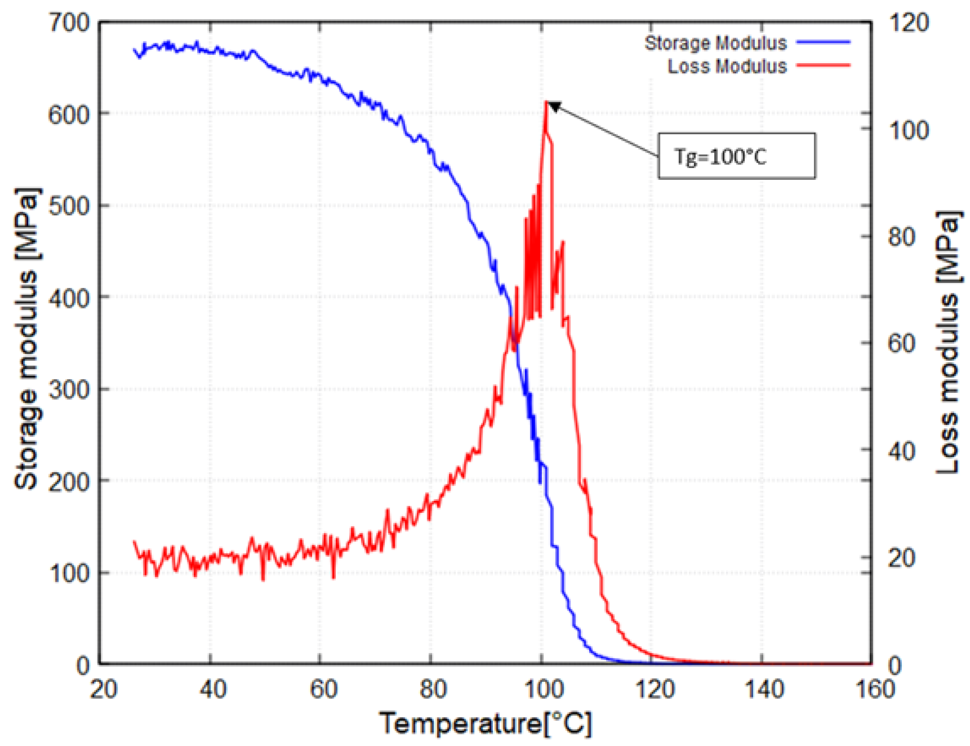
Figure 2 shows the storage and loss moduli curves versus temperature. The loss modulus increases with the decrease of the storage modulus until reaching a maximum point, and then both curves decrease. The Tg temperature value is equal to 100 °C. This value is obtained using the peak of the loss modulus curve, as illustrated in Figure 2.

3.2. Tensile Tests

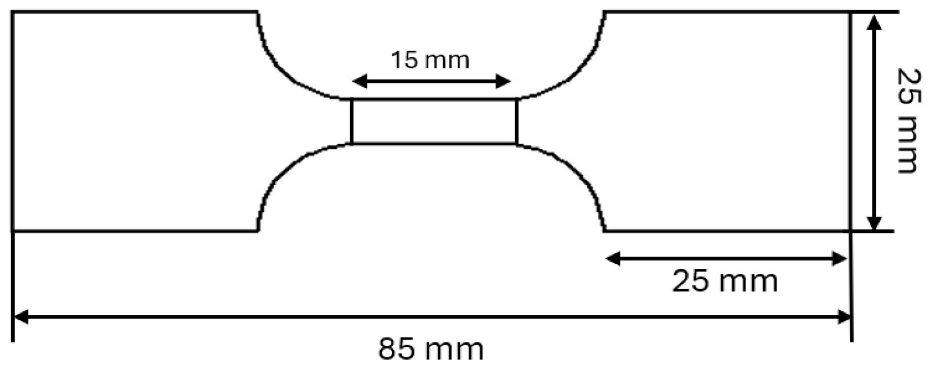
Tensile tests were conducted using the electromechanical testing machine of type INSTRON 5960 equipped with a 30 kN load cell. Displacement measurements were carried out using image correlation techniques (VIC 3D). The tensile experiments were performed at various temperatures and loading speeds. For each uniaxial tensile test, three dumbbell-shaped specimens were selected. The dimensions of the specimen are specified in Figure 3.
The diverse testing conditions and parameters employed are summarized in Table 1.
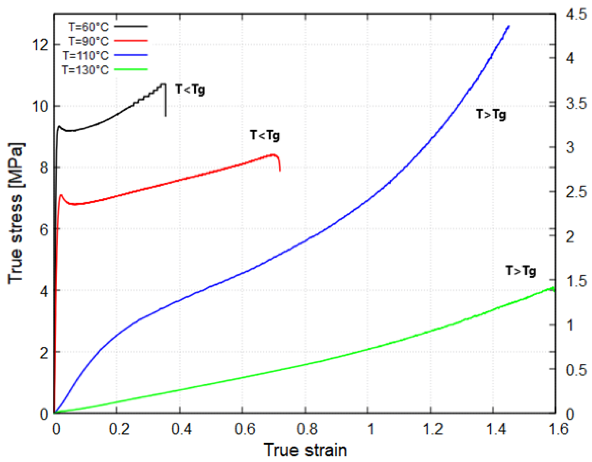
Figure 4 shows true stress–true strain curves obtained at different temperatures; these curves illustrate the temperature effect on the HIPS behavior. For temperatures below Tg, the material has a glassy behavior and deforms until failure. For temperatures above Tg, the material presents a rubbery behavior.
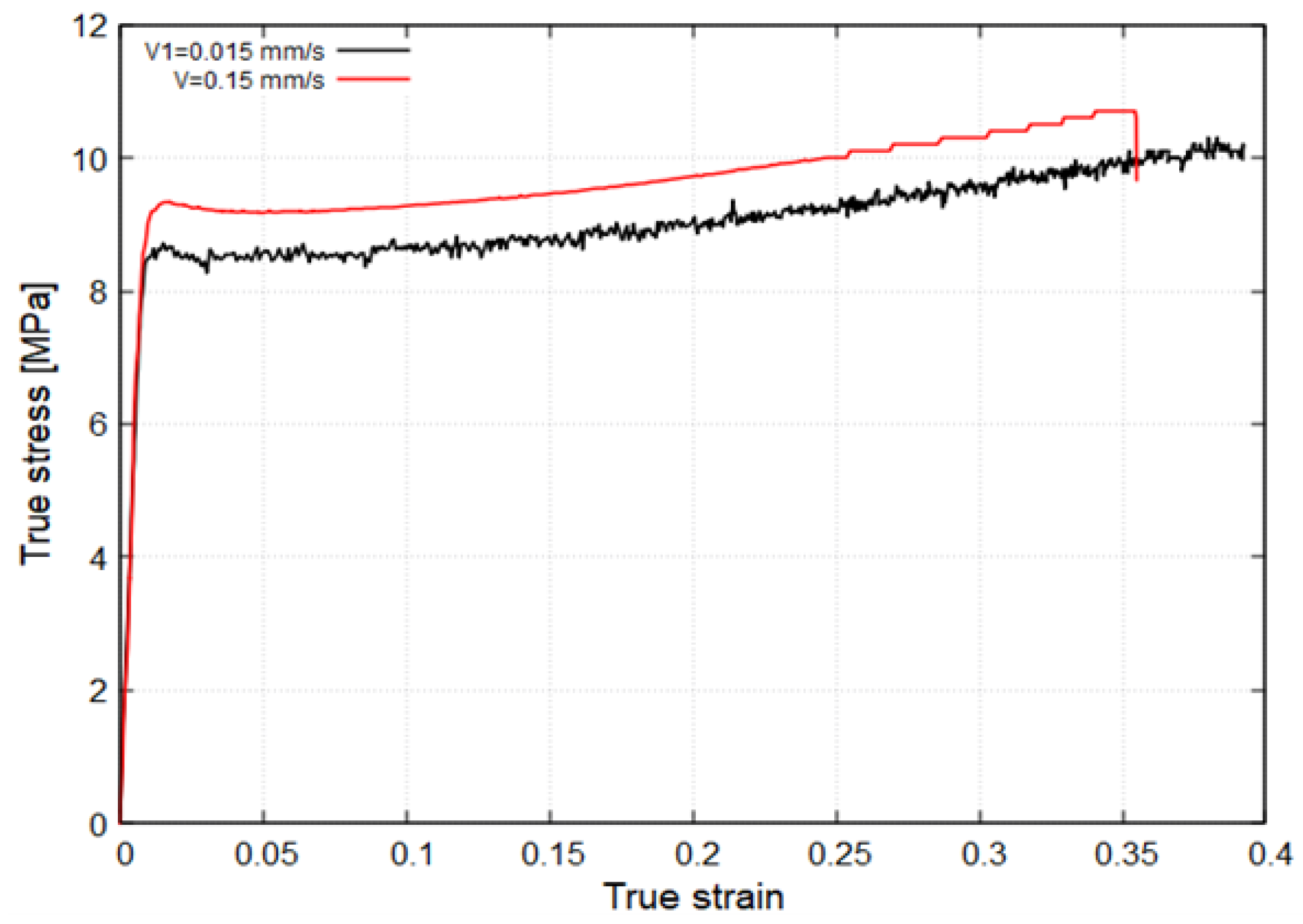
Figure 5 illustrates the effect of strain rate for a temperature test of 60 °C. It should be noted that the stress level increases with the velocity of the load.

3.3. The Constitutive Model Used in ABAQUS

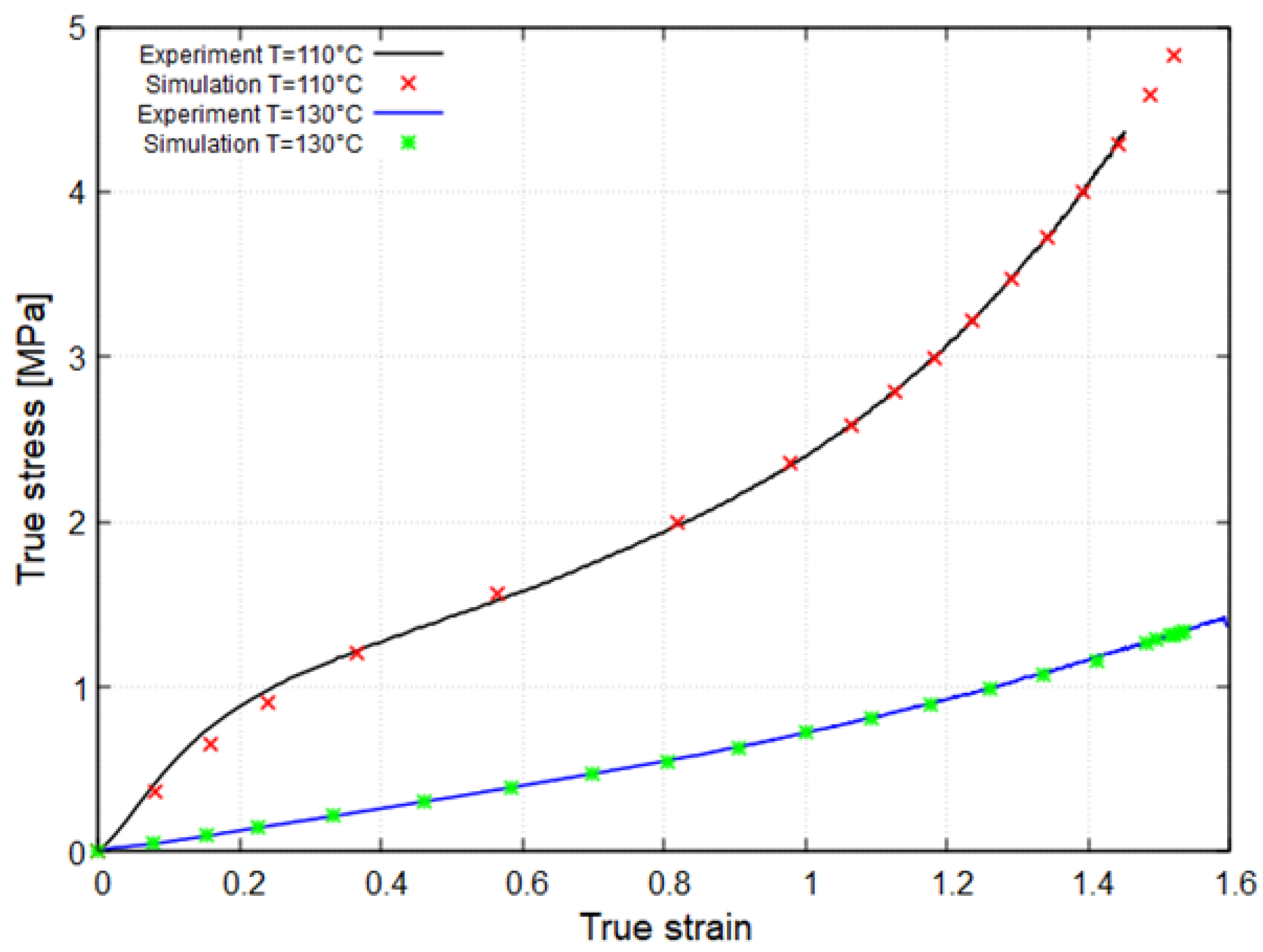
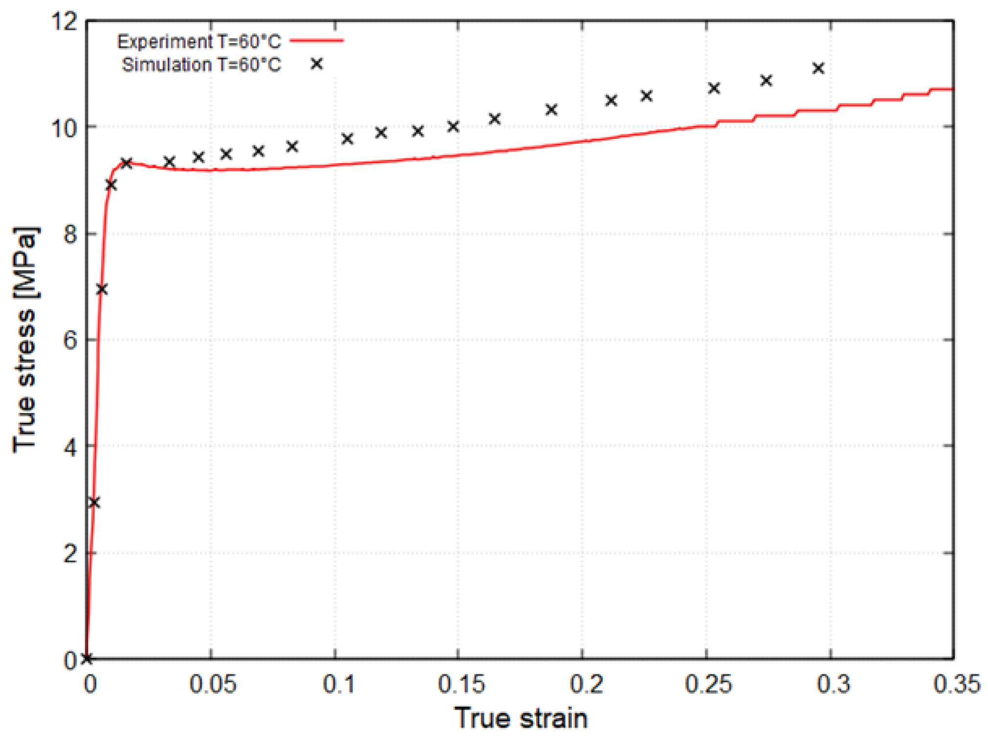
To replicate the thermo-hyperelastic behavior of the HIPS material in ABAQUS, several models are available, including the Mooney–Rivlin, Ogden, and Marlow models. The selection between these models involved simulating the uniaxial tensile test on ABAQUS using different models. A correlation was established between the experimental and numerical tests to compare the stress–strain evolution. After testing several hyperelastic models, the Marlow model was selected due to its ability to accurately predict the material behavior at temperatures both below and above Tg (the glass transition temperature). The Marlow model assumes that the strain energy potential is independent of the second deviatoric invariant I 2 . This model is defined by providing test data that characterize the deviatoric behavior. In ABAQUS, a strain energy potential is constructed based on the provided test data to precisely reproduce the material’s behavior, as shown in Figure 6 and Figure 7. The input data used to reproduce the material’s behavior as a function of temperature are shown in Table 2.
As previously mentioned, hyperelastic models do not consider the effect of the deformation rate. In this simulation, a hyper-viscoelastic coupling is used to implement the deformation rate effect.
In Abaqus, viscoelasticity can be modeled for large-strain applications as a function of reduced time for time-dependent analyses [24,25]. The viscoelastic model is defined in Abaqus using the Prony series, where the relaxation moduli are given as follows [26,27]:
G ( t ) = G + i = 1 N G i e x p ( t τ i )
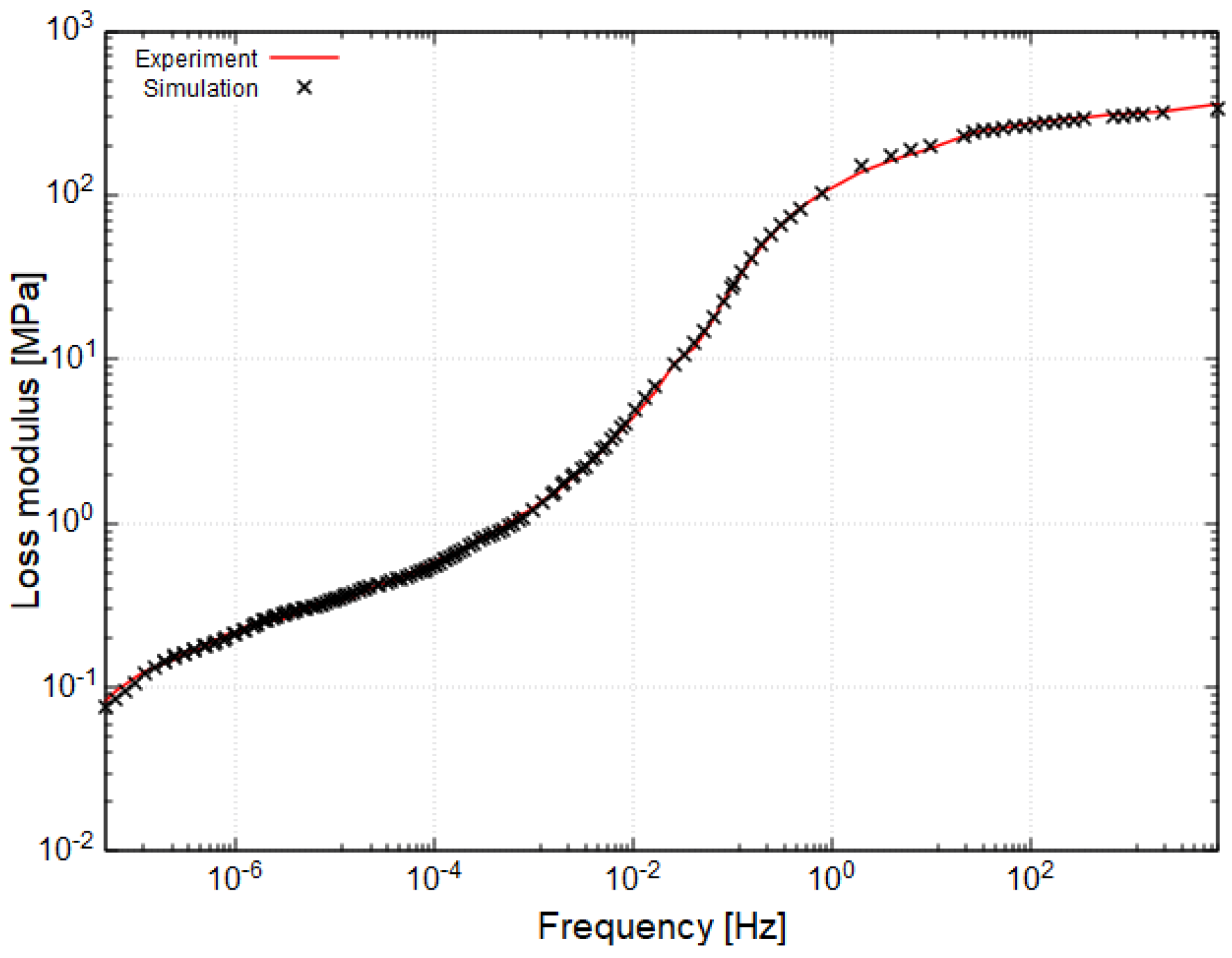
where G is the long-term modulus once the material is relaxed and τ i are the relaxation times. The parameters G , G i , and τ i have been determined through inverse identification using experimental data from DMA tests. Figure 8 and Figure 9 demonstrate a good correlation with the experimental and numerical data for loss modulus and storage modulus.
The Prony series parameters, identified as a result of this correlation, are provided in Table 3. These parameters will subsequently be utilized as input data for the FEM model.

4. Experimental–Numerical Modeling of the Industrial Demonstrator of the Thermoforming Process

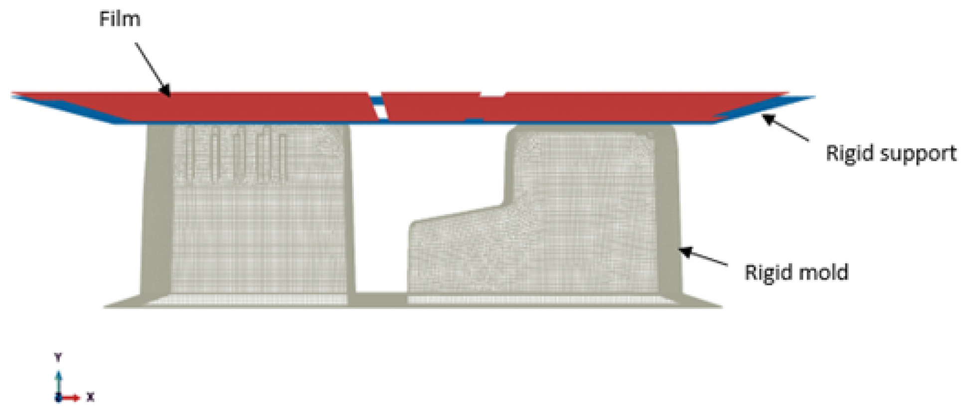
The thermoforming process of the HIPS sheet of 1.4 mm thickness was simulated numerically using the thermo-visco-hyperelastic model. As shown in Figure 10, the numerical model is made of three parts: a mold, a HIPS sheet, and a support to hold the sheet. The mold and the support were modeled as isothermal rigid bodies, incapable of deformation but capable of contact and thermal interaction with the sheet, allowing conduction in the presence of contact and even a small gap [27]. The HIPS sheet is meshed with shell elements (S4RT).
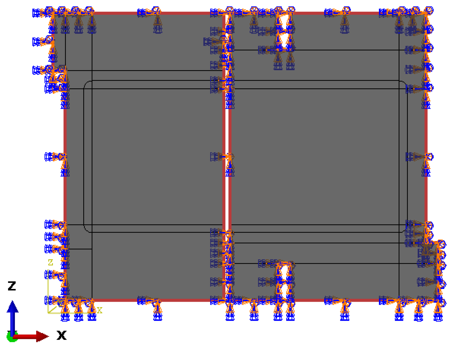
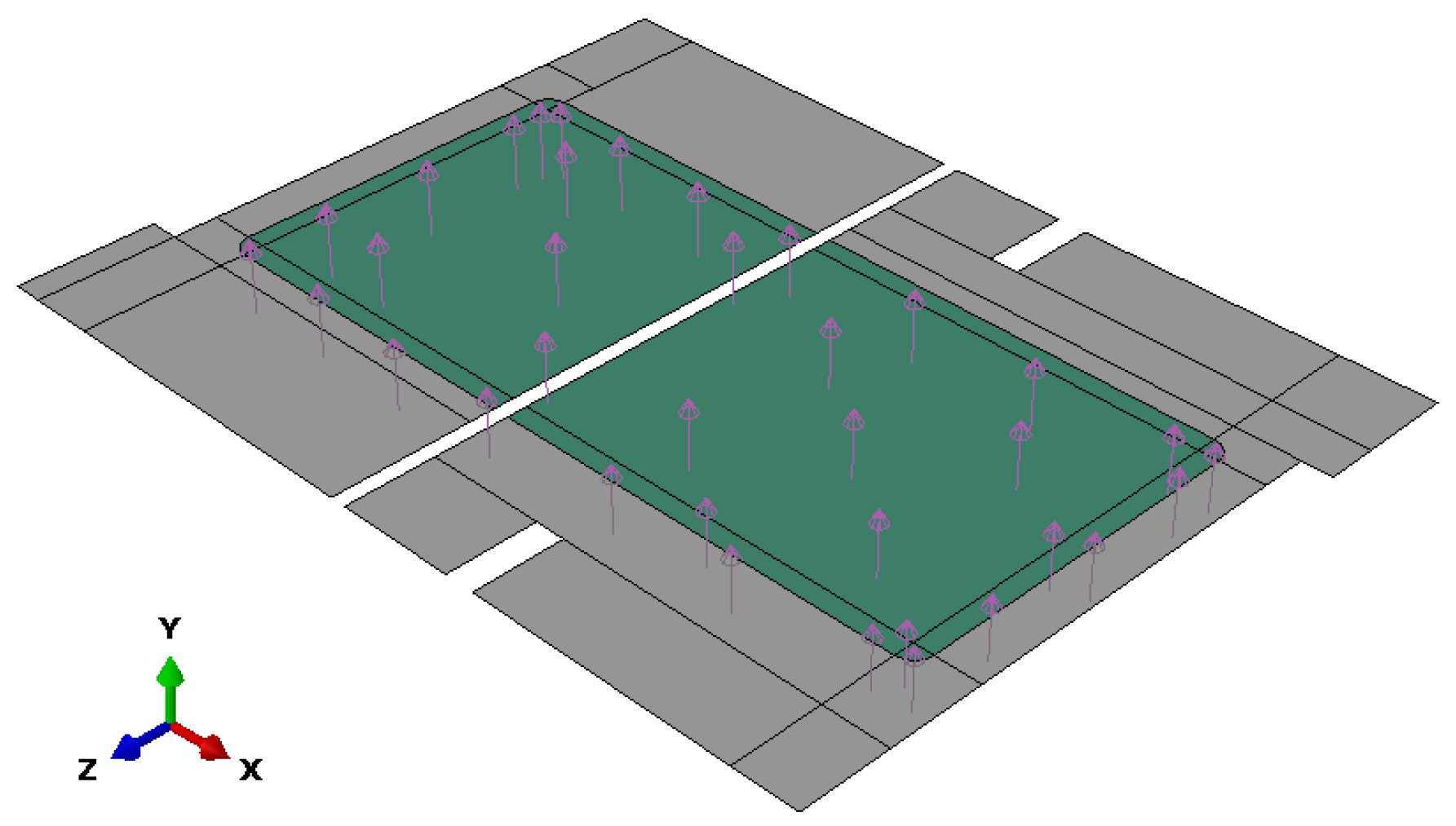
The rectangular sheet was blocked on its outboard edges, as shown in Figure 11, and a very low pressure (0.1 bar) was applied on its surface, as shown in Figure 12, for the pre-stretching step. Then, a displacement was imposed on the mold and, finally, a negative pressure was applied to the sheet so that it took the shape of the mold. The Table 4 and Table 5 provide a summary of all the boundary conditions and loads.
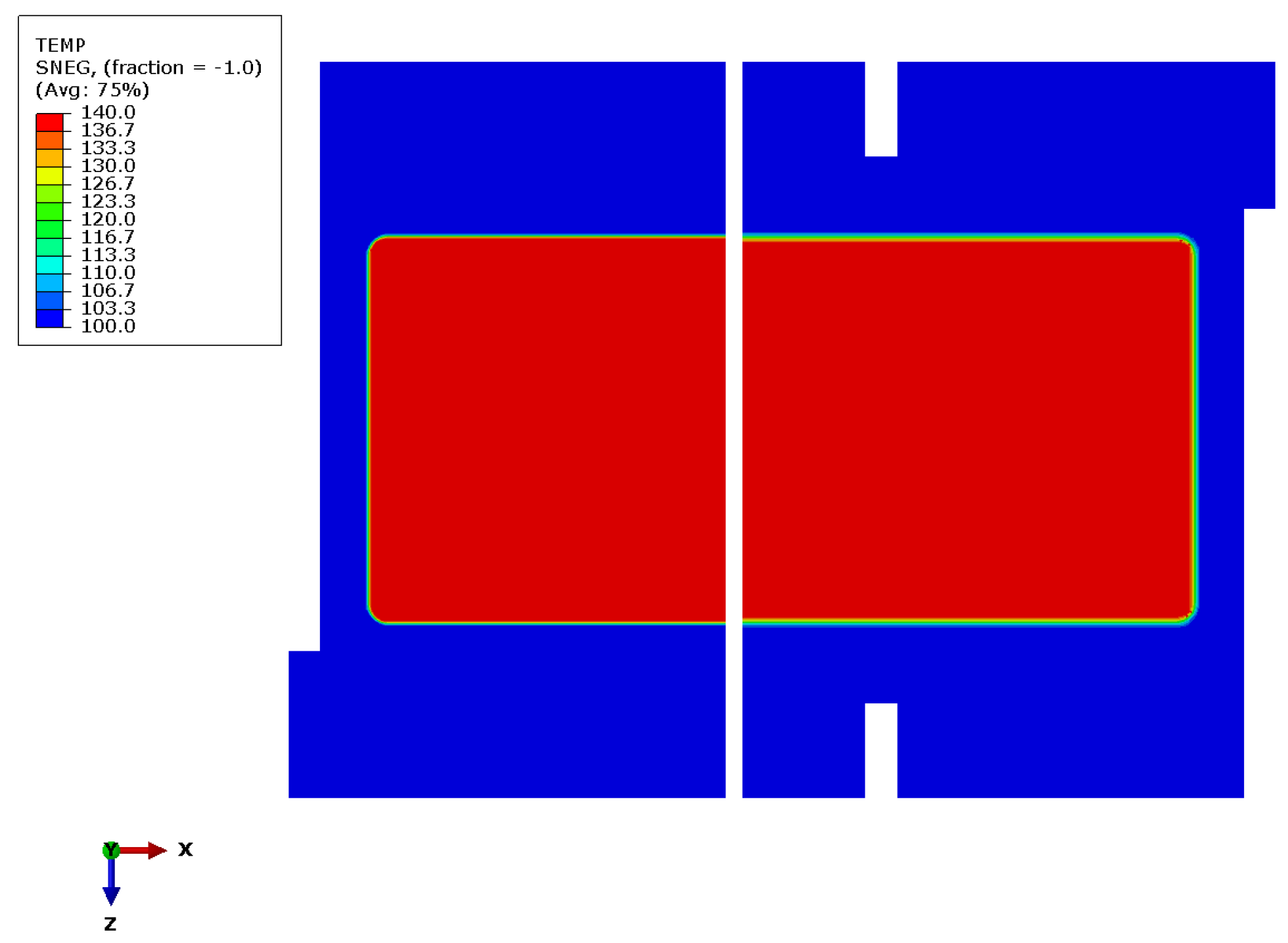
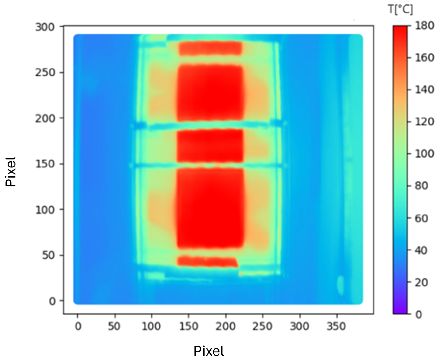
The initial temperature of the sheet was defined using the experimental values obtained using a thermal camera during the experimental test, as shown in Figure 13. Considering the real conditions of the film temperature (Figure 14), a maximum temperature was applied on the red zone of 140 °C and an average minimum temperature of 100 °C was applied on the green zone. The temperature of the mold was also imposed; it was assumed that the temperature would remain constant ( T m o l d = 50 °C). In addition, a mechanical contact was applied using a friction coefficient as well as a thermal contact using a gap conductance as mentioned in the Table 6.

5. Results and Discussion

5.1. Baseline Simulation

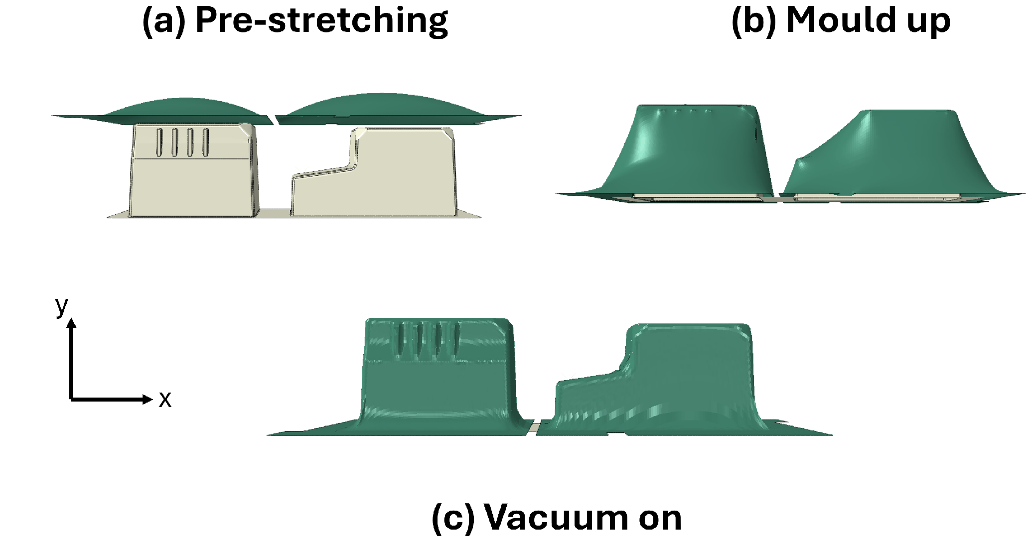
Figure 15 shows the different baseline simulations of the thermoforming process. Firstly, the HIPS sheet was formed into a bubble by applying uniform pressure (1-Pre-stretching) to improve the uniformity of thickness distribution. Then, the mold moved up until it attained its final position (two-mold moving). Finally, a negative pressure was applied on the surface of the HIPS sheet to push it against the mold (three-vacuum pressure) and to take its shape.

5.2. Temperature Distribution

Figure 16 shows the temperature distribution during the various stages of the simulation. During the pre-stretching step, the sheet is not in contact with the mold, and as a result, its temperature has not yet changed. It remains consistent with the initially imposed temperatures. For the second step, the mold comes into contact with the sheet. Due to the thermal contact, the temperature of the areas of the sheet in contact with the mold decreases. After the vacuum step is completed, all the surfaces of the sheet take on the shape of the mold, resulting in a decrease in temperature.

5.3. Stress Distribution

Figure 17 shows the von Mises stress distribution during the various stages of the simulation. The distribution of von Mises values shows a stress concentration in the first step due to boundary conditions with the fixed support. Then, for steps 2 and 3, there is a stress concentration in the areas that are most stretched by the rise of the mold.

5.4. Thickness Distribution

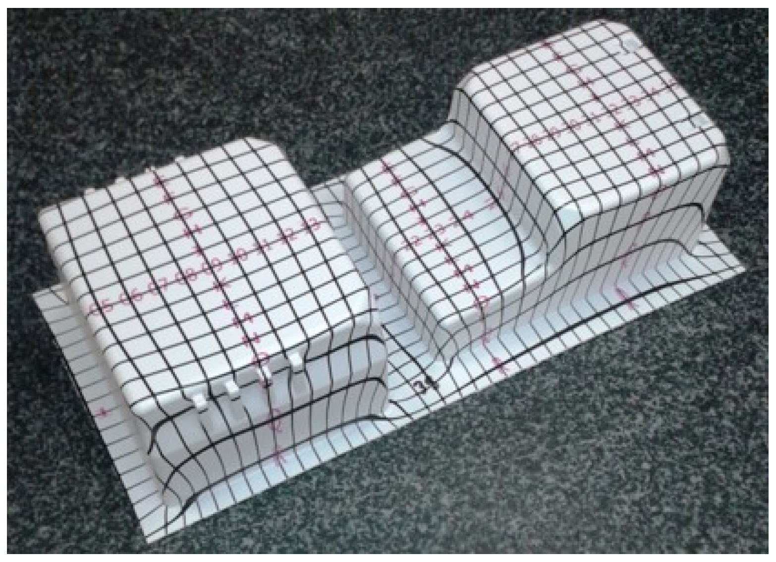
To validate the implemented numerical model, a comparison between the numerical and experimental results of the film thickness distribution was carried out. The thickness measurement points are presented below. Figure 18 shows the measurement points for the thickness of the study piece. A total of 125 pieces were used for measuring the thickness at various points. The measurement was carried out using a 3D imaging measurement machine, where a robotic measuring arm probed the piece to perform the measurement. Subsequently, an average measurement was considered for each point.
Figure 19 shows the variation of the numerical thickness on one of the lateral faces (Figure 19) of the shaped part compared to the experimental data. For the measurement points 8, 9, 10, and 11, the average percentage error was around 13%. For the rest of the points, the average relative error was 30%.
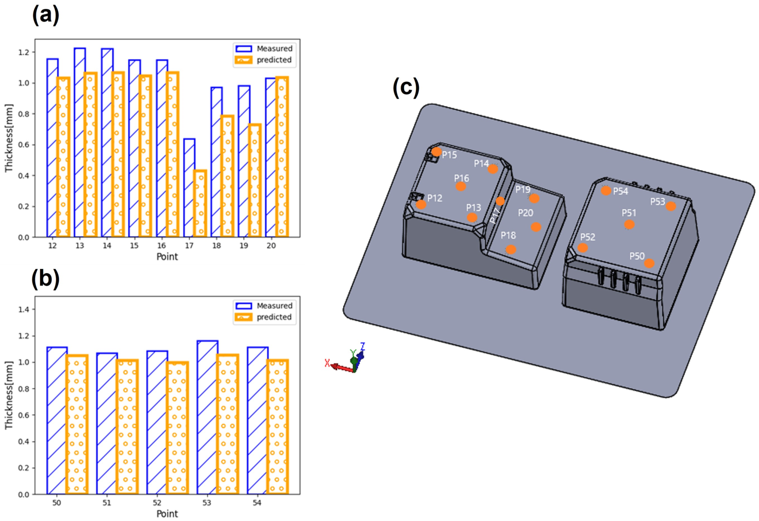
Figure 20 shows a comparison between the numerical and experimental results of the measurement points on the upper surfaces of the sheet, as shown in Figure 16c. From point 12 to 20, the average percentage error is about 14%. Figure 20 shows the evolution of the thickness for the rest of the points (50, 51, 52, 53, and 54) with an average relative error of 7%.
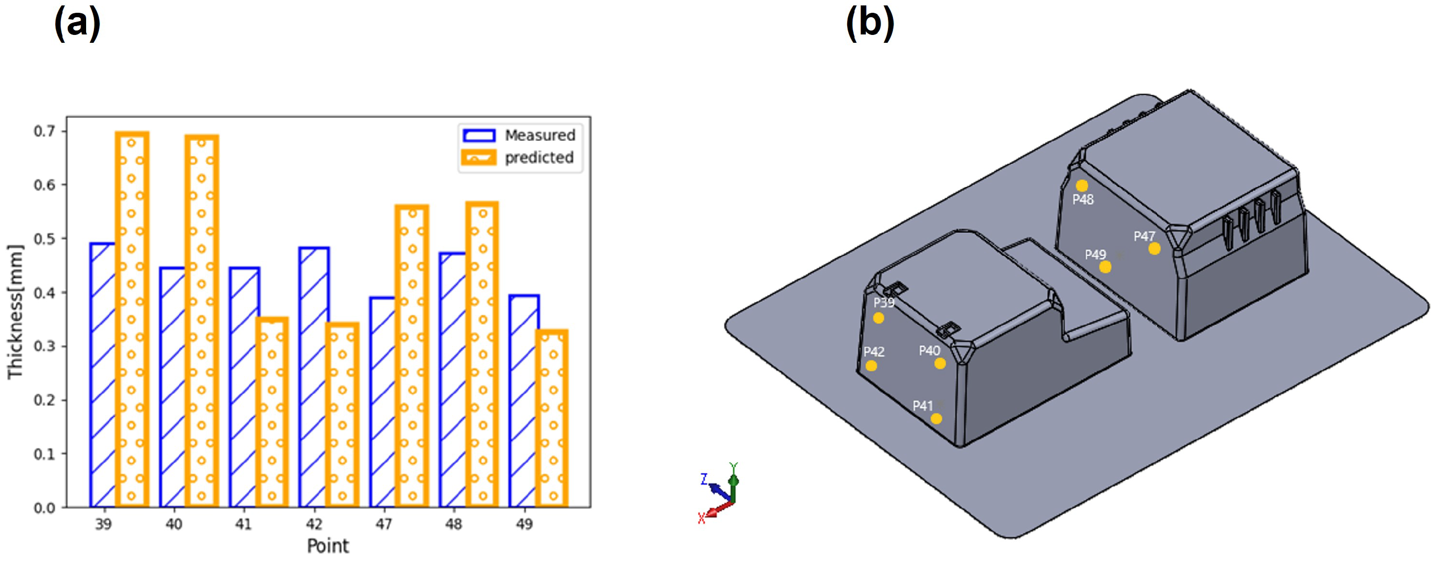
Figure 21 illustrates the evolution of the thickness for the other lateral faces of the deformed shape. In this part, the difference between the numerical and the experimental results is the highest, for an average percentage of 48%.
These results show that the error between the numerical and experimental results is lower (7%) at the upper surfaces of the deformed part. In this zone, the elements are less deformed and the temperature decreases faster compared to the evolution of the temperature in the lateral faces due to the heat transfer between the mold and the sheet. The elements at the lateral faces show a large deformation at a very high temperature, which makes the simulation more difficult and causes some stability problems. The results of our simulation are in agreement with those reported in the literature. In reference [12], a comparison was made between the numerical and experimental results for the thickness distribution of a PC sheet. A maximum error of 45% was mentioned.

6. Conclusions

In this paper, a finite element model was used to simulate the thermoforming process of an industrial demonstrator made of HIPS polymer. The HIPS behavior was evaluated by experimental uniaxial tensile tests and DMA tests. To implement the behavior of HIPS in ABAQUS finite element software, a visco-hyperelastic model, which allows for taking into account the effect of the strain rate and the temperature, was chosen. The Abaqus/Explicit solver was employed to simulate the process, where the thermal contact between the mold and the polymer sheet was included. To validate the proposed numerical model, a comparison was also carried out regarding the thickness distribution for several sections of the sheet. It was noticed that the visco-hyperelastic constitutive model can be simulated successfully. However, the nature of analysis contains both material and geometric nonlinearity, which could lead to considerable instability problems. The discrepancy between the numerical and the experimental thickness values is due to the following limitations of the constitutive model that we recommended are addressed in future works:
  • The type of mesh used in this study does not allow for using automatic selective mesh refinement to improve the deformation of a complex shape.
  • The influence of the friction coefficient on the evolution of the thickness was not studied.
  • Another important factor that was not studied is the conduction coefficient.

Author Contributions

Conceptualization, A.R., G.D., A.A., P.D. and R.L.G.; methodology, A.R., G.D., A.A., P.D. and R.L.G.; investigation, writing—original draft preparation, A.R., G.D., A.A., P.D. and R.L.G.; writing—review and editing, A.R., G.D., A.A., P.D. and R.L.G.; supervision, A.A. and R.L.G.; All authors have read and agreed to the published version of the manuscript.

Funding

This research received no external funding.

Data Availability Statement

The specifics of the literature review data can be provided upon request.

Conflicts of Interest

Authors were employed by the company Centre Technique Industriel de la Plasturgie et des Composites. The authors declare that the research was conducted in the absence of any commercial or financial relationships that could be construed as a potential conflict of interest.

References

  1. Riley, A. Plastics Manufacturing Processes for Packaging Materials. In Packaging Technology; Elsevier: Amsterdam, The Netherlands, 2012; pp. 310–360. [Google Scholar]
  2. Cha, J.; Song, H.Y.; Hyun, K.; Go, J.S. Rheological Measurement of the Nonlinear Viscoelasticity of the ABS Polymer and Numerical Simulation of Thermoforming Process. Int. J. Adv. Manuf. Technol. 2020, 107, 2449–2464. [Google Scholar] [CrossRef]
  3. Bohdan, C. Analysis of plastics packaging domestic market. Polimery 2007, 52, 811–819. [Google Scholar]
  4. Thermoformage. Plastilex. Available online: http://thermoformage-iledefrance.fr/thermoformage/ (accessed on 28 January 2024).
  5. Leite, W.D.O.; Campos Rubio, J.C.; Mata Cabrera, F.; Carrasco, A.; Hanafi, I. Vacuum Thermoforming Process: An Approach to Modeling and Optimization Using Artificial Neural Networks. Polymers 2018, 10, 143. [Google Scholar] [CrossRef] [PubMed]
  6. McCool, R.; Martin, P.J. The Role of Process Parameters in Determining Wall Thickness Distribution in Plug-Assisted Thermoforming. Polym. Eng. Sci. 2010, 50, 1923–1934. [Google Scholar] [CrossRef]
  7. Collins, P.; Lappin, J.F.; Harkin-Jones, E.M.A.; Martin, P.J. Effects of Material Properties and Contact Conditions in Modelling of Plug Assisted Thermoforming. Plast. Rubber Compos. 2000, 29, 349–359. [Google Scholar] [CrossRef]
  8. Hosseini, H.; Berdyshev, B.V.; Mehrabani-Zeinabad, A. A Solution for Warpage in Polymeric Products by Plug-Assisted Thermoforming. Eur. Polym. J. 2006, 42, 1836–1843. [Google Scholar] [CrossRef]
  9. Makradi, A.; Ahzi, S.; Belouettar, S.; Ruch, D. Thermoforming Process of Semicrystalline Polymeric Sheets: Modeling and Finite Element Simulations. Polym. Sci. Ser. 2008, 50, 550–557. [Google Scholar] [CrossRef]
  10. Atmani, O.; Abbès, B.; Abbès, F.; Li, Y.M.; Batkam, S. Identification of a thermo-elasto-viscoplastic behavior law for the simulation of thermoforming of high impact polystyrene. AIP Conf. Proc. 2018, 1960, 120003. [Google Scholar] [CrossRef]
  11. Dong, Y.; Lin, R.J.T.; Bhattacharyya, D. Finite Element Simulation on Thermoforming Acrylic Sheets Using Dynamic Explicit Method. Polym. Polym. Compos. 2006, 14, 307–328. [Google Scholar] [CrossRef]
  12. Takaffoli, M.; Hangalur, G.; Bakker, R.; Chandrashekar, N. Thermo-Visco-Hyperelastic Behavior of Polycarbonate in Forming of a Complex Geometry. J. Manuf. Process. 2020, 57, 105–113. [Google Scholar] [CrossRef]
  13. Arruda, E.M.; Boyce, M.C. Three-Dimensional Constitutive Model for the Large Stretch Behavior of Rubber Elastic Materials. J. Mech. Phys. Solids 1993, 41, 389–412. [Google Scholar] [CrossRef]
  14. Atmani, O.; Abbès, B.; Abbès, F.; Lid, Y.M.; Batkam, S. Etude expérimentale et numérique de l’influence de la température et de la vitesse de déformation sur le thermoformage assisté par poinçon du polystyrène. In Proceedings of the 24th French Mechanics Congress, Aachen, Germany, 9–13 September 2019. [Google Scholar]
  15. Sánchez, E.; Nájera, A.; Sotomayor, O. Numerical Study of the Viscoelastic Mechanical Response of Polystyrene in the Process of Thermoforming through the Generalized Maxwell Model. Mater. Today Proc. 2022, 49, 107–114. [Google Scholar] [CrossRef]
  16. Erdogan, E.S.; Eksi, O. Prediction of Wall Thickness Distribution in Simple Thermoforming Moulds. J. Mech. Eng. 2014, 60, 195–202. [Google Scholar] [CrossRef]
  17. Fu, M.W.; Wang, J.L. Size Effects in Multi-Scale Materials Processing and Manufacturing. Int. J. Mach. Tools Manuf. 2021, 167, 103755. [Google Scholar] [CrossRef]
  18. Tao, F.; Cheng, J.; Qi, Q.; Zhang, M.; Zhang, H.; Sui, F. Digital Twin-Driven Product Design, Manufacturing and Service with Big Data. Int. J. Adv. Manuf. Technol. 2018, 94, 3563–3576. [Google Scholar] [CrossRef]
  19. Tobajas, R.; Elduque, D.; Javierre, C.; Ibarz, E.; Gracia, L. A Comparative Study of Hyperelastic Constitutive Models for an Automotive Shaft Seal Material. Int. J. Serv. Comput. Oriented Manuf. 2018, 3, 171–189. [Google Scholar] [CrossRef]
  20. Boukamel, A. Modélisation Mécaniques et Numériques des Matériaux et Structures en éLastomères. HDR Thesis, Universite De La Mediterranee (Aix-Marseille II), Marseille, France, 2010. [Google Scholar]
  21. Hyperelastic Behavior of Rubberlike Materials. Abaqus Documentation 2017. Available online: https://classes.engineering.wustl.edu/2009/spring/mase5513/abaqus/docs/v6.6/books/usb/default.htm?startat=pt05ch17s01abo16.html (accessed on 28 January 2024).
  22. Abaqus Documentation, Hyperelastic Material Models in Abaqus. Available online: https://classes.engineering.wustl.edu/2009/spring/mase5513/abaqus/docs/v6.6/books/key/default.htm?startat=ch20abk03.html (accessed on 28 January 2024).
  23. Bergström, J. Elasticity/Hyperelasticity. In Mechanics of Solid Polymers; William Andrew: Norwich, NY, USA, 2015. [Google Scholar]
  24. Time Domain Viscoelasticity. Abaqus Documentation 2017. Available online: https://classes.engineering.wustl.edu/2009/spring/mase5513/abaqus/docs/v6.6/books/usb/default.htm?startat=pt05ch17s07.html (accessed on 28 January 2024).
  25. Chae, S.-H.; Zhao, J.-H.; Edwards, D.R.; Ho, P.S. Characterization of the Viscoelasticity of Molding Compounds in the Time Domain. J. Electron. Mater. 2010, 39, 419–425. [Google Scholar] [CrossRef]
  26. Finite-Strain Viscoelasticity. Abaqus Documentation 2017. Available online: https://classes.engineering.wustl.edu/2009/spring/mase5513/abaqus/docs/v6.6/books/stm/default.htm?startat=ch04s08ath127.html (accessed on 28 January 2024).
  27. O’Connor, C.P.J.; Menary, G.; Martin, P.J.; McConville, E. Finite Element Analysis of the Thermoforming of Polypropylene. Int. J. Mater. Form. 2008, 1, 779–782. [Google Scholar] [CrossRef]
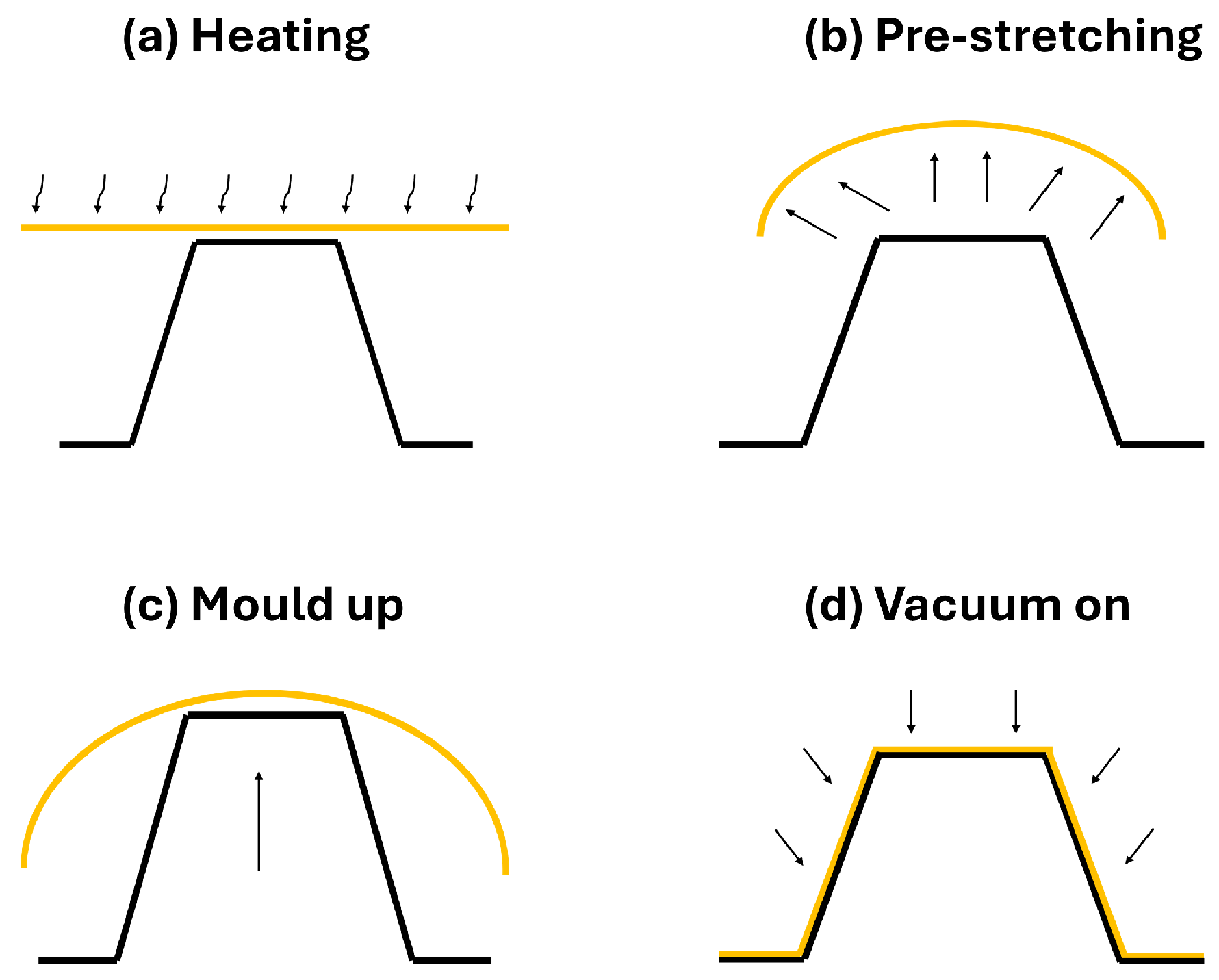
Figure 1. Thermoforming process: (a) heating: the sheet is heated using radiant heat until it reaches the optimal temperature for thermoforming; (b) pre-stretching: the sheet is mechanically stretched before molding, ensuring uniform thickness; (c) mold up: the mold goes up until it touches the film; (d) vacuum on: vacuum pressure is used to remove air from under the sheet and ensure close contact with the mold contours.
Jmmp 08 00033 g001
Figure 2. DMA test results for HIPS.
Jmmp 08 00033 g002
Figure 3. The dimensions of a dumbbell-shaped specimen for the tensile test.
Jmmp 08 00033 g003
Figure 4. Experimental tensile curves of HIPS at different temperatures and a velocity of 0.15 mm/s.
Jmmp 08 00033 g004
Figure 5. Experimental tensile curves of HIPS at different velocities and temperature tests of 60 °C.
Jmmp 08 00033 g005
Figure 6. Comparison of experimental and numerical tensile curves at different temperatures above Tg.
Jmmp 08 00033 g006
Figure 7. Comparison of experimental and numerical tensile curves at temperature test below Tg.
Jmmp 08 00033 g007
Figure 8. Correlation of experimental and numerical loss modulus curves.
Jmmp 08 00033 g008
Figure 9. Correlation of experimental and numerical storage modulus curves.
Jmmp 08 00033 g009
Figure 10. Different parts of assembly.
Jmmp 08 00033 g010
Figure 11. Boundary condition: blocking the film.
Jmmp 08 00033 g011
Figure 12. Pressure application area.
Jmmp 08 00033 g012
Figure 13. Initial temperature conditions.
Jmmp 08 00033 g013
Figure 14. Distribution of experimental temperature values of the plate obtained through an IR camera.
Jmmp 08 00033 g014
Figure 15. Steps of the numerical simulation. (a): the sheet is mechanically stretched before molding, ensuring uniform thickness. (b): the mold goes up until it touches the film. (c): vacuum pressure is used to remove air from under the sheet and ensure close contact with the mold contours.
Jmmp 08 00033 g015
Figure 16. (a) Distribution of sheet temperature during the pre-stretching step, (b) distribution of sheet temperature during the mold up step, and (c) distribution of sheet temperature during the vacuum on step.
Jmmp 08 00033 g016
Figure 17. (a) Distribution of von Mises stress during the pre-stretching step, (b) distribution of von Mises stress during the mold-up step, and (c) distribution of von Mises stress during the vacuum on the step.
Jmmp 08 00033 g017
Figure 18. Meshed demonstrator used for experimental thickness measurement.
Jmmp 08 00033 g018
Figure 19. (a) Thickness distribution on side 1. (b) Experimental measurement points of the thickness on side 1.
Jmmp 08 00033 g019
Figure 20. (a,b) Thickness distribution on side 2. (c) Experimental measurement points of the thickness on side 2.
Jmmp 08 00033 g020
Figure 21. (a) Thickness distribution on side 3. (b) Experimental measurement points of the thickness on side 3.
Jmmp 08 00033 g021
Table 1. Uniaxial tensile tests as a function of temperature and loading speed.
Temperature [°C]Test SpecimensLoading Speeds [mm/s]
6030.015–0.15
9030.015–0.15
11030.15–1.5–15
12030.15–1.5–15
13030.15–1.5–15
14030.15–1.5–15
Table 2. Material input data as a function of temperature used in FEM.
Temperature [°C]Input DataCurve Used
60Experimental test dataNominal stress–strain curve
90Experimental test dataNominal stress–strain curve
110Experimental test dataNominal stress–strain curve
120Experimental test dataNominal stress–strain curve
130Experimental test dataNominal stress–strain curve
140Experimental test dataNominal stress–strain curve
Table 3. Prony series parameters for FEM model.
Term Number g i τ i [s]
1 31 × 10 5 104 × 10 4
2 32 × 10 5 94 × 10 4
3 37 × 10 5 10 4
4 10 3 10 3
5 3 × 10 3 97
6 18 × 10 3 9.9
7 17 × 10 2 94 × 10 2
8 27 × 10 2 10 1
9 14 × 10 2 10 2
10 17 × 10 2 10 4
Table 4. Loading conditions.
StepPressure [Bar]Displacement [mm]Duration [s]
Pre-stretching0.01-0.5
Mould up-1022
Vacuum on1-2
Table 5. Contact conditions.
Contact TypePartsProperties
Mechanical contactSheet and moldHard contact and friction coefficient (f = 0.3)
Thermal contactSheet and moldGap conductance 1
1 The data are given below.
Table 6. Gap conductance parameters.
Conductance [ mW mm 2 · C ]Clearance [mm]
100
50.005
2.50.01
1.660.015
1.250.02
10.025
00.05
Disclaimer/Publisher’s Note: The statements, opinions and data contained in all publications are solely those of the individual author(s) and contributor(s) and not of MDPI and/or the editor(s). MDPI and/or the editor(s) disclaim responsibility for any injury to people or property resulting from any ideas, methods, instructions or products referred to in the content.