The Optimization of Machining Parameters for Milling Operations by Using the Nelder–Mead Simplex Method

Abstract

The purpose of machining operations is to make specific shapes or surface characteristics for a product. Conditions for machining operations were traditionally selected based on geometry and surface finish requirements. However, nowadays, many researchers are optimizing machining parameters since high-quality products can be produced using more expensive and advanced machines and tools. There are a few methods to optimize the machining process, such as minimizing unit production time or cost or maximizing profit. This research focused on maximizing the profit of computer numerical control (CNC) milling operations by optimizing machining parameters. Cutting speeds and feed are considered as the main process variables to maximize the profit of CNC milling operations as they have the greatest effect on machining operation. In this research, the Nelder–Mead simplex method was used to maximize the profit of CNC milling processes by optimizing machining parameters. The Nelder–Mead simplex method was used to calculate best, worst, and second-worst value based on an initial guess. The possible range of machining parameters was limited by several constraints. The Nelder–Mead simplex method yielded a profit of 3.45 ($/min) when applied to a commonly used case study model.

1. Introduction

Machining operations are used to produce shapes or surface characteristics for a product. Some common conventional machining operations are turning, boring, drilling, reaming, milling, and tapping. Conditions for machining operations were chosen based on geometry and surface finish requirements rather than profit when costs were comparatively low on labor, resource, machines, and tools. However, nowadays, many researchers proposed optimizing machining parameters to maximize profit when using expensive modern machine tools.

Milling processes have rotating cutters to make specific shapes or surface characteristics by eliminating material from the workpiece. There are two basic milling operations, as shown in Figure 1, namely peripheral (end) milling and face milling. Peripheral milling is usually used for profiling or slotting works, and face milling is required for making flat surfaces of a workpiece [1]. Milling processes were used to test an optimization method in this study.

There are many ways to optimize the machining process, such as minimizing production unit time, minimizing production cost, or maximizing profit.

Karandikar and Kurfess [2] used machining costs to optimize milling operations based on tool life. They described an approach for experimental design for tool life testing and machining cost optimization using surrogate modeling and the value of information method. They found that the proposed approach can be utilized in an industrial setting without explicitly modeling tool life, and it is better in predicting tool life than the traditional statistical design of experiments such as factorial designs and central composite design.

Li et al. [3] examined energy saving for multi-objective machining with consideration of the energy consumption by optimizing machining parameters for the cutting process. They defined a relationship between cutting parameters and energy consumption in the machining process. They analyzed the energy consumption and production rate with sets of optimized and unoptimized cutting parameters for different objectives. They found that the objectives of low consumed energy and high production rate can be obtained simultaneously by optimizing cutting parameters.

Chen et al. [4] were able to optimize machining parameters with a reduction in energy consumption and production time for the face milling process. They presented an integrated approach for minimizing the energy footprint and production time by optimizing cutting tools and cutting parameters. Three energy footprint-aware optimization models were used to demonstrate the necessity of the integrated approach. In model 1, the cutting tool-related parameters were preset according to the machining handbook. In model 2, the cutting tool-related parameters were optimized through the Cuckoo algorithm with feasible cutting parameters. In model 3, the integrated optimization of the cutting tool and parameters was used. When the energy footprint of each model was compared, the integrated approach achieved the most energy-efficient footprint. Therefore, they found that it is necessary to optimize the cutting tool and cutting parameters in an integrated manner.

Faisal and Kumar [5] researched the optimization of machining process parameters in Electric Discharge Machining (EDM) by using the Particle Swarm Optimization (PSO) and Biogeography-Based Optimization (BBO) techniques. The PSO technique took initialization with a population of random solutions and then updating the generations to achieve an optimal solution. The BBO technique optimizes a function stochastically and iteratively. They found that the BBO method improved the material removal rate and reduced surface roughness.

Abbas et al. [6] researched surface roughness optimization of AZ61 magnesium alloy finish turning by using a novel Edgeworth–Pareto optimization of an Artificial Neural Network (ANN). Cutting parameters were optimized for minimum surface roughness. When they compared the theoretical and experimental results, the reliability of ±1.35% was achieved.

An approach for maximizing the profit of CNC milling operations was proposed by Tolouei and Bidhendi [7] without exceeding constraints, such as maximum machine power and maximum cutting forces, for each milling operation. Tolouei and Bidhendi [7] suggested using empirical and mechanistic functions to estimate the profit of CNC milling operations.

The profit for CNC milling operations generally consists of production cost, production time, and the sale price of a product. The production cost per part is made up of several components, including raw material cost, overhead cost, tool changing cost, machining cost, and setup cost. Setup, material, and overhead costs are not dependent on the selection of machining parameters. Machining cost tends to decrease with increasing cutting speed, while tool changing cost tends to increase with higher cutting speeds. Even though low cutting speeds and feed tend to increase tool life, they will produce a rough surface finish [8].

Production time per part is made up of several components, including machining time, tool changing time, and setup time. Contrary to the production cost, machining time decreases with increasing cutting speeds and feed, but this results in increasing tool wear. However, gains in the material removal rate with increased cutting speeds, feed, and depth of cut are accompanied by decreasing tool life [9]. Kant and Sangwan [10] investigated the effect of cutting speeds and feed. They observed that cutting forces and vibrations decrease with high cutting speeds, but high feed causes vibration and heat generation. Therefore, determining the proper cutting speed and feed was the most crucial issue in this paper.

As shown in Figure 1, feed is the distance machined by a tool at each revolution of a tool during the machining operation. The depth of cut is defined as the thickness of metal removed from a workpiece through the radial or axial direction [11]. The rotational speed of the spindle determines the cutting speed, which can be expressed as the tangential speed of a cutting tool, regardless of machining operation. Since the optimum depth of cut is dependent on the interaction between the cutting tool, the geometry of the product, and workpiece material, it is usually a fixed value and not a candidate for optimization. Therefore, the cutting speed and feed were considered machining parameters in this study [1].

The optimization of CNC machining processes using machine learning and numerical algorithms is a key way to eliminate unnecessary testing, and it will result in saving time, material wastage, and effort. We expect that the Nelder–Mead Simplex method, when applied to optimize machining parameters of the CNC milling operation, will yield a higher profit accurately and rapidly.

2. Materials and Methods

2.1. State of the Art

Tolouei and Bidhendi [7] have established an objective function with penalty functions through a case study. They presented an optimization model that is non-linear with multiple variables and multiple constraints. Tolouei and Bidhendi [7] optimized the case study using the method of feasible direction, and feasible starting points were determined by the machining handbooks. The case study proposed by Tolouei and Bidhendi [7] was subsequently used by researchers such as Yildiz [12], Abhishek [13], Deepak [14], Gomez and Jurado [15], and Zhai et al. [16] utilizing different optimization methods.

Yildiz [12] used the Cuckoo search algorithm and Hybrid Differential Evolution Algorithm to optimize the machining processes. Abhishek [13] employed the Genetic Algorithm to optimize the machining parameters of milling operations. Deepak [14] used Particle Swarm Optimization (PSO) to optimize the machining process. Gomez and Jurado [15] utilized a modified Shuffled Frog-Leaping Algorithm to find the optimal machining parameters in milling processes. Zhai et al. [16] used a Novel Teaching–Learning-Based Optimization Algorithm with a dynamic assignment learning strategy (DATLBO) to select the optimum machining parameters in multi-tool milling operations. In this research, the Nelder–Mead simplex method [17] was utilized to optimize the milling process using the same case study in Tolouei and Bidhendi [7] to determine whether a better solution can be achieved.

2.2. Research Gap

It can be observed from the above literature review that optimization methods such as the Cuckoo search, the Hybrid Differential Evolution Algorithm, the Genetic Algorithm, Particle Swarm Optimization, and Shuffled Frog-Leaping have mostly been used for the optimization of machining parameters. However, these methods are restricted to find a solution rapidly and cheaply, and if these methods are applied to a more complex optimization problem, it will take more time and effort. The Nelder–Mead simplex method is more robust in comparison to other methods mentioned above because it uses feasible individuals instead of functional derivatives. In this research paper, the Nelder–Mead simplex method was adopted to optimize machining parameters such as the cutting speed (m/min) and feed (mm/tooth).

2.3. The Nelder–Mead Simplex Method

The Nelder–Mead simplex method [17] can be used to minimize a mathematical function by evaluating the result. This method is especially employed for non-linear problems for which the derivatives may not be known. The Nelder–Mead simplex method usually has effective and computational compact procedures. In n + 1 dimensional space, when x₁, …, x_n, x_n+1 are given, this space can be defined “simplex”, where f(x_i) is a function value at x_i. When i and j are different, each function value can be written by x_i and x_j, and the centroid point between these values can be defined by C. To find the optimum value when variables change, there are three operations. Reflection, contraction, and expansion were used to find an optimum value [16].

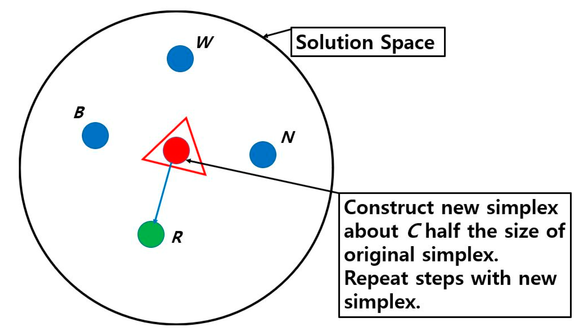
Starting from an initial value, results calculated in each reflection, contraction, and expansion algorithm are classified into best (B), worst (W), and next worst (N) values. Equation (4) was used to terminate the simplex loop as the stopping criteria when the calculated value was below the value of stopping criteria [18]. In the reflection process, as shown in Figure 2, a new higher point presented by R, and the reflection function can be represented by:

$$R=\left(1+\alpha \right)C-B$$

(1)

where α is the reflection coefficient and a positive constant. f(R) is a new value at point R. If the R variable exists between B and W, the reflection process would be started again with the new simplex, but if a new R is less than W, R is denoted by W, and f(R) can be replaced by f(W). If R obtained for reflection step does not meet the criteria, the expansion step is used with the expansion coefficient, γ. When f(R) is greater than f(W) and the expansion process fails, then N should be replaced by R before restarting the expansion process:

$$E=\left(1+\gamma \right)R-\gamma C$$

(2)

where f(R) is bigger than f(B) for all i ≠ B, R can be replaced by B as a new maximum value. According to the new maximum value, the contraction process can be represented by:

$$C_{con}=\beta R+\left(1+\beta \right)C$$

(3)

The contraction coefficient β should be a number between 0 and 1. In the contraction algorithm, results are classified into best (B), worst (W), and next worst (N) values. The contraction algorithm continues until the next best result is smaller than the previous best value. Before restarting the process, new x_i should be replaced by (x_i + W)/2. A failed contraction is much rarer but can occur when a valley is curved, and one point of the simplex is much farther from the valley bottom than the others [16]. The operations of reflection, contraction, and expansion are not significantly affected by the change in coefficient α, β, and γ. The Nelder–Mead simplex method in this study used the standard coefficients, α = 1, β = 2, γ = 0.5, and σ = 0.5. The operation is stopped when f(x_i) falls below the criteria value. The stopping criteria equation is defined by:

$$f\left(x_i\right)<\sqrt{\frac{1}{n+1}{\displaystyle \sum }_{i=1}^{n+1}{[f(x_i)-f\left(C\right)]}^2}$$

(4)

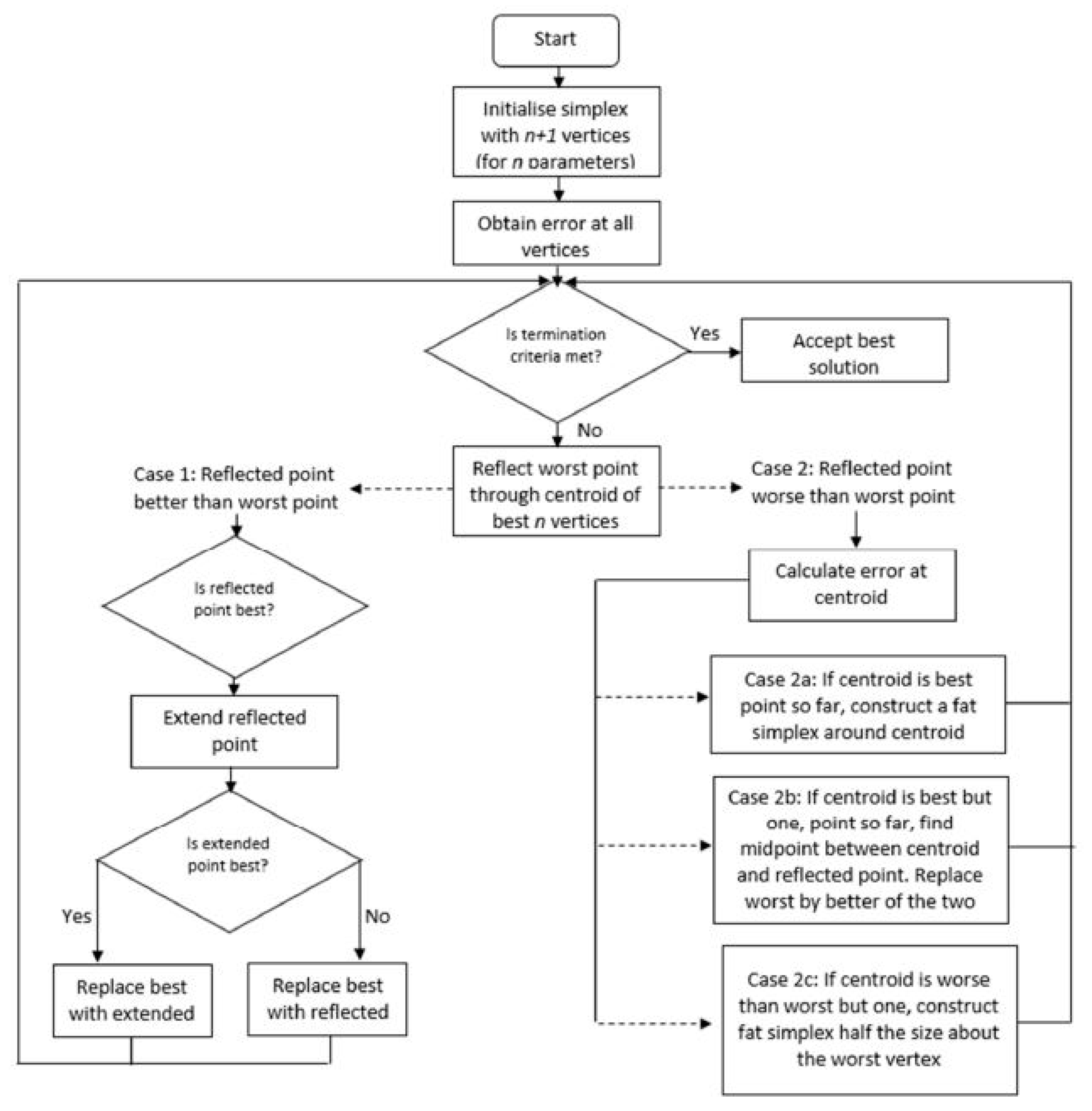
The Nelder–Mead simplex method is used to find the best, worst, and second-worst values through employing a large range of values; this process is illustrated in a flow chart shown in Figure 3. In practice, some variables need to be limited through the constraints. The Nelder–Mead simplex algorithm with constraints was programmed by MATLAB software. The hardware was a 2.80 GHz Intel Core i7 processor, with 8 GB of memory.

2.4. Adaptive Penalty Function

The penalty function method is commonly used for optimizing a constrained objective function. In this paper, a self-adaptive penalty function was used because (a) it allows us to employ infeasible individuals efficiently, (b) the method is simple to utilize, and (c) it does not need parameter tuning. Feasible individuals of the objective function are the values satisfying all of the constraints. If one of the individuals does not satisfy at least one of the constraints, that individual is called an infeasible individual [19].

$$F\left(x\right)=d\left(x\right)+p\left(x\right)$$

(5)

F(x), a new fitness value called distance value is calculated by the sum of the infeasible individuals, d(x) in the normalized fitness constraint violation space, and two penalized values, p(x). The best infeasible individuals in the current populations can be found in the algorithm.

2.4.1. d(x), Distance Value

The distance value of the objective function, d(x), is calculated by:

$$d\left(x\right)=\{\begin{array}{cc}\hfill v\left(x\right),& \mathrm{if} r_f=0\hfill \\ \hfill \sqrt{f^{″}\left(x^2\right)+v\left(x^2\right)},& \mathrm{otherwise}\hfill \end{array}$$

(6)

where

$$r_f=\frac{\mathrm{the}\mathrm{number}\mathrm{of}\mathrm{feasible}\mathrm{individuals}}{\mathrm{population}\mathrm{size}}$$

(7)

To calculate the distance value of the objective function, the smallest and the largest values represent f_min and f_max, respectively. Then $f^{\prime }\left(x\right)$, a new distance value, is updated by:

$$f^{\prime }\left(x\right)=f\left(x\right)-f_{\min }$$

(8)

where f(x) is a value of the objective function. Then the new distance value is normalized by:

$$f^{″}\left(x\right)=\frac{f^{\prime }\left(x\right)}{f_{\max }-f_{\min }}$$

(9)

Then v(x), the constraint violation of each infeasible individual, is calculated by:

$$v\left(x\right)=\frac{1}{m}{\displaystyle \sum }_{j=1}^m\frac{c_j\left(x\right)}{c {\max }_j}$$

(10)

where

$$c_j\left(x\right)=\{\begin{array}{cc}\hfill \max \left(0,g_j\left(x\right)\right),& j=1, \dots , k\hfill \\ \hfill \max \left(0,\left|h_j\left(x\right)\right|-\delta \right),& j=k+1, \dots , m\hfill \end{array}$$

$g_j$ is the type of inequality constraint and $h_j$ is the type of equality constraint. δ is a tolerance value, and m is the total number of constraints. In this paper, a tolerance of ${10}^{-12}$ and m of 3 were used.

2.4.2. p(x), Two Penalties

Two penalties are used to decrease the infeasible individuals in the population and identify the best feasible individuals in the population. p(x), the two penalties, are defined by:

$$p\left(x\right)=\left(1-r_f\right)X\left(x\right)+r_{f}Y\left(x\right)$$

(11)

where

$$\begin{gathered} X\left(x\right)=\{\begin{array}{cc}\hfill 0,& \mathrm{if} r_f=0\hfill \\ \hfill v\left(x\right),& \mathrm{otherwise}\hfill \end{array} \\ Y\left(x\right)=\{\begin{array}{cc}\hfill 0,& \mathrm{if} x \mathrm{is} \mathrm{a} \mathrm{feasible} \mathrm{individual}\hfill \\ \hfill f^{″}\left(x\right),& \mathrm{if} x \mathrm{is} \mathrm{an} \mathrm{infeasible} \mathrm{individual}\hfill \end{array} \end{gathered}$$

In two penalties, X(x) has more impact than Y(x), since X(x) is supposed to have a large value for individuals with a large number of constraint violations when there are few feasible individuals in the population.

2.5. Objective Models

Machining parameters, such as the depth of cut, feed, and the cutting speed, have significant effects on the machining operation. However, the depth of cut is generally predetermined by the geometry of a workpiece and operation sequence. Therefore, a proper cutting speed and feed combination will be determined to minimize unit cost and time. The fundamental model describing the profit of producing a workpiece through machining operation is described as follows [7]:

$$P_r=\frac{S_p-C_u}{T_u}$$

(12)

2.5.1. Unit Cost

Unit cost is the total cost of making a unit of the product, which can be broken into four separate groups: the cost of the raw material, setup cost, machining cost, and tool changing cost [7].

$$C_u=C_{mat}+\left(C_l+C_o\right)t_s+\left(C_l+C_o\right)t_m+\left(C_l{t}_{tc}+C_t+C_o{t}_{tc}\right)\frac{t_m}{T}$$

(13)

where

$$\{\begin{array}{c}{C}_{mat}=\mathrm{The} \mathrm{cost} \mathrm{of} \mathrm{the} \mathrm{raw} \mathrm{material}\\ C_l{t}_s=\mathrm{Setup} \mathrm{cost} \mathrm{for} \mathrm{preparing} \mathrm{a} \mathrm{workstation}\\ C_o{t}_s=\mathrm{Overhead} \mathrm{cost}\\ C_l{t}_{tc}=\mathrm{Labor} \mathrm{cost} \mathrm{for} \mathrm{changing} \mathrm{a} \mathrm{tool}\\ C_t=\mathrm{The} \mathrm{cost} \mathrm{of} \mathrm{a} \mathrm{cutting} \mathrm{tool}\\ C_o{t}_{tc}=\mathrm{Overhead} \mathrm{cost} \mathrm{for} \mathrm{changing} \mathrm{a} \mathrm{tool}\end{array}$$

There is some indirect cost that cannot be neglected in preparation for machining operations. These small costs are calculated by overhead cost, C_ot_s. Tool changing costs are calculated by the sum of corresponding labor, overhead, and tool cost. Roughly, the unit cost can be defined by the sum of all these costs. Equation (13) is for a single tool, and it can be extended to multiple tools.

2.5.2. Machining Time

The machining time equation used in Tolouei and Bidhendi [7] is:

$$t_m=\frac{k}{f_r}=\frac{k}{fN}=\frac{k}{f_{t}zN} with N=\frac{1000V}{\pi d}$$

(14)

However, overtravel distance should be considered to determine the total tool travel distance. The addition of the overtravel distance will likely decrease the profit, as the tool is spending more time moving in the machining envelope. The machining time equation, considering the overtravel distance, can be redefined as [20]:

$$t_m=\frac{k+\epsilon }{f_r}=\frac{k+\epsilon }{fN}=\frac{k+\epsilon }{f_{t}zN} with N=\frac{1000V}{\pi d}$$

(15)

where

$$\{\begin{array}{c}k=\mathrm{Travel} \mathrm{distance} \mathrm{of} \mathrm{each} \mathrm{tool}\\ \epsilon =\mathrm{Overtravel} \mathrm{distance} \mathrm{of} \mathrm{each} \mathrm{cutter}\\ f_r=\mathrm{Feed} \mathrm{per} \mathrm{minute} (\mathrm{mm}/\min )\\ f_t=\mathrm{Feed} (\mathrm{mm}/\mathrm{tooth})\\ N=\mathrm{Spindle} \mathrm{speed} (\mathrm{rev}/\min )\\ V=\mathrm{Cutting} \mathrm{speed} (\mathrm{m}/\min )\\ d=\mathrm{Cutter} \mathrm{diameter} \left(\mathrm{mm}\right)\end{array}$$

This equation is simplified to:

$$t_m=\frac{k+\epsilon }{f_{t}zN}=\frac{d\pi \left(k+\epsilon \right)}{1000z}{f_t}^{-1}{V}^{-1}=K_1{f}_t{}^{-1}{V}^{-1}$$

(16)

where a new constant K₁ is defined as:

$$K_1=\frac{d\pi \left(k+\epsilon \right)}{1000z}$$

(17)

2.5.3. Tool Life

Increasing the cutting speed and feed results in excessive heat generation that causes tool wear at both flank and rake face of a tool. Contrary to excessive process parameters, insufficient cutting speeds and feed will lead to low profit. Kronenberg [21] and Boothroyd [20] proposed the specific relationship between tool life and cutting parameters of a tool as:

$$T=\frac{60}{Q}{\left[\frac{c_s{\left(G/5\right)}^g}{A^{w}V}\right]}^{\frac{1}{n}}$$

(18)

where V, c_s, and A represent the cutting speed, the cutting speed constant, and chip cross-sectional area, respectively. G is the slenderness ratio, while g, n, and w are exponents of the slenderness ratio, tool life, and chip cross-sectional area, respectively. The quality of a tool and workpiece material determines the cutting speed constant and tool life exponent values. The high-quality tool and workpiece material usually have a higher value for c_s, g, and n. Tool life is negatively affected by the high level of workpiece hardness, the cutting speed, and feed. Iqbal et al. [8] noted that the workpiece hardness has more influence on tool life than the cutting speed and feed. In Equation (18), chip cross-sectional area, A, is af_tz, and slenderness ratio, G, is a/f_tz, respectively. Therefore, Equation (18) is redefined by:

$$T=\frac{60}{Q}{\left[\frac{c_s{\left(a/5f_{t}z\right)}^g}{{\left(a{f}_t\right)}^{w}V}\right]}^{\frac{1}{n}}$$

(19)

Similar to K₁, K₂ can be grouped in a constant as:

$$K_2=\frac{60}{Q}{\left[\frac{c_s{\left(a/5z\right)}^g}{{\left(az\right)}^w}\right]}^{\frac{1}{n}}$$

(20)

Then, the tool life equation is simplified to:

$$T=K_2{V}^{-\frac{1}{n}}{f}_t{}^{-\frac{\left(w+g\right)}{n}}$$

(21)

To calculate tool life correctly, an engaged cutting edge should be considered the proportion of tool contact with a workpiece per revolution. For the milling process used in this study, the proportion of tool contact with a workpiece per revolution, Q, can be determined by [20]:

for step milling,

$$Q_1=\frac{1}{\pi }\arcsin \frac{a_{rad}}{d}$$

(22)

for side milling,

$$Q_2=\frac{1}{4}+\frac{1}{2\pi }\arcsin (\frac{a_{rad}}{d}-1)$$

(23)

for slot milling,

$$Q_3=\frac{1}{2}$$

(24)

The ratio between machining time and tool life, t_m/T, can be defined as:

$$\frac{t_m}{T}=\frac{K_1{f}_t{}^{-1}{V}^{-1}}{K_2{V}^{-\frac{1}{n}}{f}_t{}^{-\frac{\left(w+g\right)}{n}}}$$

(25)

Defining K₃ = K₁/K₂, the ratio machining time per tool life equation, t_m/T is simplified to:

$$\frac{t_m}{T}=K_3{V}^{\left(\frac{1}{n}-1\right)}{f}_t{}^{\left(\frac{w+g}{n}-1\right)}$$

(26)

Equations (16) and (26) are plugged into the general cost per unit Equation (13).

$$\begin{array}{c}{C}_u=C_{mat}+\left(C_l+C_o\right)t_s+\left(C_l+C_o\right)K_1{f}_t{}^{-1}{V}^{-1}+(C_l{t}_{tc}+C_t\\ +C_o{t}_{tc})K_3{V}^{\left(\frac{1}{n}-1\right)}{f}_t{}^{\left(\frac{w+g}{n}-1\right)}\end{array}$$

(27)

Equation (27) is the unit cost equation for a machining process that only involves a single tool, and it is represented as a function of machining parameters, such as the cutting speed and feed. As regards multi-tool operations, tool changing time should be considered as multi-machining operations are needed. Equation (27) can be transformed to the i-th term up to m operations, where t_tci is the tool changing time, and C_ti is the cost of each cutting tool.

$$\begin{gathered} C_u=C_{mat}+\left(C_l+C_o\right)t_s+{\displaystyle \sum }_{i=1}^m\left(C_l+C_o\right)K_{1i}{f}_{ti}{}^{-1}{V}_i{}^{-1} \\ +{\displaystyle \sum }_{i=1}^m{C}_{ti}{K}_{3i}{V}_i{}^{\left(\frac{1}{n}-1\right)}{f}_{ti}{}^{\left(\frac{w+g}{n}-1\right)}+{\displaystyle \sum }_{i=1}^m\left(C_l+C_o\right)t_{tci} \end{gathered}$$

(28)

Unit cost equation for multi-tool operations can be simplified to:

$$C_u=C_{mat}+\left(C_l+C_o\right)t_s+{\displaystyle \sum }_{i=1}^m{c}_{1i}{f}_{ti}{}^{-1}{V}_i{}^{-1}+{\displaystyle \sum }_{i=1}^m{c}_{2i}{V}_i{}^{\left(\frac{1}{n}-1\right)}{f}_{ti}{}^{\left(\frac{w+g}{n}-1\right)}+{\displaystyle \sum }_{i=1}^m{c}_{3i}$$

(29)

where C_mat, C_l, C_o, and t_s represent the cost of the raw material per part, the cost of setting up the tool, overhead cost, and setup time, respectively. In the production unit cost equation, several constant parameters can be grouped by c_1i, c_2i, and c_3i.

$$c_{1i}=\left(C_l+C_o\right)K_{1i}$$

(30)

$$c_{2i}=C_{ti}{K}_{3i}$$

(31)

$$c_{3i}=\left(C_l+C_o\right)t_{tci}$$

(32)

C_mi, the minimum production cost during multi-milling operations, can be optimized by considering raw material, setup, and tool changing costs, which were not considered during the optimization of the multi-tool machining process.

$$C_{mi}={\displaystyle \sum }_{i=1}^m{c}_{1i}{f}_{ti}{}^{-1}{V}_i{}^{-1}+{\displaystyle \sum }_{i=1}^m{c}_{2i}{V}_i{}^{\left(\frac{1}{n}-1\right)}{f}_{ti}{}^{\left(\frac{w+g}{n}-1\right)}$$

(33)

2.6. Unit Time

Unit time, T_u, is the time required to make a part. The unit time equation for a single tool proposed by Tolouei and Bidhendi [7] is:

$$T_u=t_s+t_m+t_{tc}\left(\frac{t_m}{T}\right)$$

(34)

The unit time equation is composed of setup time, t_s, machining time, t_m, and tool changing time, t_tc, respectively. The equation for t_m and t_m/T has been derived in the unit cost section. The equation t_tc(t_m/T) is used to calculate tool changing time, which could occur due to the tool wear during machining operation, substituting Equations (16) and (26) in Equation (34):

$$T_u=t_s+\frac{d\pi \left(k+\epsilon \right)}{1000z}{f}_t{}^{-1}{V}^{-1}+t_{tc}\left(K_3{V}^{\left(\frac{1}{n}-1\right)}{f}_t{}^{\left(\frac{w+g}{n}-1\right)}\right)$$

(35)

and for multiple tools, it becomes:

$$T_u=t_s+{\displaystyle \sum }_{i=1}^m{K}_{1i}{f}_{ti}{}^{-1}{V}_i{}^{-1}+{\displaystyle \sum }_{i=1}^m{t}_{tci}\left(K_3{V}_i{}^{\left(\frac{1}{n}-1\right)}{f}_{ti}{}^{\left(\frac{w+g}{n}-1\right)}\right)$$

(36)

2.7. Profit

$$P_r=\frac{S_p-C_u}{T_u}$$

(37)

In Equation (37), S_p, T_u, and C_u refer to the sale price of a component, unit time, and unit cost, respectively. If feed and the cutting speed increase, unit time decreases, due to increasing the metal removal rate. However, that results in increasing unit costs. Therefore, great balance between the cutting speed and feed is required within constraints, such as maximum machine power, surface finish requirements, and maximum cutting forces. Equation (38) was used as an objective function in this work. Equations (29) and (36) are plugged into Equation (37).

$$P_r=\frac{S_p-(C_{mat}+\left(C_l+C_o\right)t_s+{{\displaystyle \sum }}_{i=1}^m{c}_{1i}{f}_{ti}{}^{-1}{V}_i{}^{-1}-{{\displaystyle \sum }}_{i=1}^m{c}_{2i}{V}_i{}^{\left(\frac{1}{n}-1\right)}{f}_{ti}{}^{\left(\frac{w+g}{n}-1\right)}+{{\displaystyle \sum }}_{i=1}^m{c}_{3i})}{t_s+{{\displaystyle \sum }}_{i=1}^m{K}_{1i}{f}_{ti}{}^{-1}{V}_i{}^{-1}+{{\displaystyle \sum }}_{i=1}^m{t}_{tci}\left(K_3{V}_i{}^{\left(\frac{1}{n}-1\right)}{f}_{ti}{}^{\left(\frac{w+g}{n}-1\right)}\right)}$$

(38)

As the objective function varies significantly with the cutting speed and feed during its machining operation, the profit should be calculated for each operation:

$$P_{ri}=\frac{R_i-C_{mi}}{t_{mi}}$$

(39)

This model of optimization is very helpful in verifying the effects of input data. C_mi is the machining cost of the i-th operation, and t_mi is the machining time of the i-th operation. C_mi and t_mi, respectively, can be represented by:

$$C_{mi}=c_{1i}{f}_{ti}{}^{-1}{V}_i{}^{-1}+c_{2i}{V}_i{}^{\left(\frac{1}{n}-1\right)}{f}_{ti}{}^{\left(\frac{w+g}{n}-1\right)}$$

(40)

and

$$t_{mi}=K_{1i}{f}_{ti}{}^{-1}{V}_i{}^{-1}$$

(41)

R_i is the money earned by a workshop at each operation except raw material, setup, and tool changing costs. R_i can be defined by:

$$R_i=R\frac{t_{mi}}{t_m}$$

(42)

where

$$R=S_p-\left(C_{mat}+\left(C_l+C_o\right)t_s+{\displaystyle \sum }_{i=1}^m{c}_{3i}\right)$$

(43)

2.8. Constraints

The constraints are developed by using mechanical knowledge of milling operations, which is derived from published papers and empirical data. There are several constraints suggested by Rad [22] to limit machining parameters. For this study, the cutting speed and feed were limited by several constraints, such as

• Maximum machine power,
• Surface finish requirement,
• Maximum cutting force permitted by the rigidity of the tool,
• Available feed and spindle speed on the machine tool, and
• Heat generated by cutting.

The cutting fluid has significant effects that (a) reduce cutting temperature, (b) improve the accuracy of machining, and (c) reduce the tool–chip contact length. The coolants are used to achieve better accuracy of machining by reducing the temperature of the tool and workpiece because low temperatures contribute to lower thermal expansion of the workpiece and tool [23]. This study will assume that coolant is used all the time, so heat generation was neglected. Therefore, maximum machine power, surface finish requirements, and maximum cutting force were considered as the main constraints. In the following section, mathematical models of the constraint were defined, and these constraints were used to find the optimum value of the objective function as the boundary conditions.

2.8.1. Maximum Machine Power

Due to the advancement of CNC machine capacities, the available power of CNC machines has increased. Maximum machine power was used as a constraint to limit feed and the cutting speed. MDC [24] proposed the machining power equation, P, that can be calculated by:

$$P=\frac{P_c}{e}=\frac{k_c{Q}_v}{e}$$

(44)

where k_c, Q_v, and e represent specific cutting force depending on the workpiece material, metal removal rate, and machine tool efficiency factor, respectively.

Q_v, Metal Removal Rate

Q_v, the metal removal rate, was defined by MDC [24]:

$$Q_v=f_r{a}_{rad}a=\frac{1000z{a}_{rad}a{f}_{t}V}{\pi d} with N=\frac{1000V}{\pi d}$$

(45)

where f_t, z, a_rad, a, and V represent the feed, the tooth number of each tool, radial depth of each cut, axial depth of each cut, and the cutting speed of each operation, respectively. Equation (44) can be transformed into Equation (46) when Equation (45) is plugged into Equation (44).

$$P=\frac{1000k_c{a}_{rad}az{f}_{t}V}{\pi de}$$

(46)

The machining power of each operation should not exceed the available motor power, P_m. Therefore, the power constraint can be written as:

$$c_{4}V{f}_t\le 1$$

(47)

where

$$c_4=\frac{1000k_c{a}_{rad}az}{\pi de{P}_m}$$

(48)

e, Machine Tool Efficiency Factor

The machine tool efficiency factor was classified depending on the type of drive. The machine tool efficiency factor is listed in

Table 1. e, Machine tool efficiency factor [24].

Type of Drive	e	Type of Drive	e
Direct belt drive	0.90	Geared head drive	0.70–0.80
Back gear drive	0.75	Oil hydraulic drive	0.60–0.90

following the type of drive.

2.8.2. Surface Finish Requirement

The roughness average (R_a) is the arithmetic average of the roughness profile ordinates, and it can be used to quantify the quality of a machined surface, where surface quality is critical and needs a characterizing indicator. Wear, friction, lubrication, fatigue, etc., have been analyzed corresponding to R_a (μm), because it is a useful guideline of surface texture for describing the surface’s functional nature [25]. During machining operation, surface finish is affected by feed, the diameter of a cutter, type of milling operation, run out of cutter forces, tool conditions, and spindle run out. Among the variables, feed proved to have the highest effect on surface finish. Gains in the contact area between the workpiece and the cutting tool with increased feed and depth of cut are accompanied by increasing surface roughness [26]. In the case of a perpendicular tooth, the arithmetic average value of surface finish in plain milling and end milling can be represented by Equation (49) [27]:

$$R_a=318\frac{f_t{}^2}{4d}$$

(49)

and in face milling, by Equation (50) [27]:

$$R_a=318\frac{f_t}{\tan \left(la\right)+\cot \left(ca\right)}$$

(50)

where la and ca represent the lead angle of a tool and the clearance angle of a tool, respectively. Required surface finish, R_a, must not exceed the maximum attainable surface finish, R_a(at), under the conditions. Therefore, the surface finish for end milling becomes:

$$c_5{f}_t{}^2\le 1$$

(51)

where

$$c_5=\frac{318}{4d{R}_{a\left(at\right)}}$$

(52)

and for face milling

$$c_6{f}_t\le 1$$

(53)

where

$$c_6=\frac{318}{R_{a\left(at\right)}\left[\tan \left(la\right)+\cot \left(ca\right)\right]}$$

(54)

In the case of a round tooth, surface finish in milling is also affected by a lot of factors that do not present in turning, and these factors result mainly from differences in tooling and process kinematics. For face milling, surface finish depends on an insert radius and effective feed. In the feed direction, the average surface finish can be calculated approximately by using formulas. As regards a round tooth, the arithmetic value of surface finish in face milling can be represented by [1]:

$$R_a=\frac{0.0312f_t{}^2}{r_c}$$

(55)

Required roughness, R_a, must not surpass the maximum attainable surface finish, R_a(at), under the conditions. Therefore, the surface finish for the round tool becomes:

$$c_7{f}_t{}^2\le 1$$

(56)

where

$$c_7=\frac{0.0321}{R_{a\left(at\right)}{r}_c}$$

(57)

2.8.3. Cutting Forces

In the machining process, sufficient cutting forces should be applied to overcome the resistance of the material. Subramanian et al. [28] found that increasing a chip cross-sectional area by increasing feed and depth of cut is accompanied by increasing cutting forces. A high cutting speed has a minor effect on cutting forces when low feed and axial depth of cut are used. Cutting force is the most important criteria when examining machining performance. The total cutting force applied to a cutting tool is the result of tangential, feed, and radial forces. The total cutting force, F_c, resulting from machining operation must not exceed the permitted cutting force, F_c(per). Permitted values of cutting forces have been introduced by tool manufacturers for different tools. These force values are determined from Equation (58), due to calculating forces experimentally.

$$F_c={\left[{\left(F_T\right)}^2+{\left(F_F\right)}^2+{\left(F_R\right)}^2\right]}^{1/2}$$

(58)

where F_F, F_T, and F_R represent feeding, radial, and tangential forces, respectively [29]. Since the individual components of the cutting forces on the right-hand side of Equation (58) cannot be measured easily, cutting force is usually calculated by multiplying chip cross-sectional area and exponent values. Approximately, the total cutting force equation can be defined by:

$$F_c=k_{c}a{f}_{t}z$$

(59)

where k_c value is the specific cutting force of a workpiece. Total cutting force, F_C, resulting from machining operation must not exceed permitted cutting force, F_c(per). Therefore, the constraint of cutting force can be defined by:

$$k_{c}a{f}_{t}z\le F_{c \left(per\right)}$$

(60)

This equation can be simplified by:

$$c_8{f}_t\le 1$$

(61)

where

$$c_8=k_{c}az/F_{c \left(per\right)}$$

(62)

2.9. Case Study

A case study suggested by Tolouei and Bidhendi [7] was used to optimize machining processes with the Nelder–Mead simplex method. Machining operations are conducted with a type of machine and constant values listed in

Table 2. Parameters for case study [7].

Type	Vertical CNC Milling Machine (Pm = 8.5 kW)
e	95%
Workpiece material	10L50 leaded steel (225 BHN)
Cmat ($)	0.5
Sp ($)	25
Co ($/min)	1.45
Cl ($/min)	0.45
cs of HSS tool	33.98
cs of carbide tool	100.05
g (unitless)	0.14
n of HSS tool	0.15
n of carbide tool	0.3
ts (min)	2
ttc (min)	0.5
kc (MPa)	1800
Kp (W)	2240
W (unitless)	1.1
w (unitless)	0.28

,

Table 3. Required machining operation for case study [14].

Operation No	Operation Type	Tool No	a (mm)	k (mm)	ε (mm)	Ra (μm)	Fc(per) (kN)
1	Face milling	1	10	450	35	2	156.5
2	Corner milling	2	5	90	7	6	17.1
3	Pocket milling	2	10	450	7	5	17.1
4	Slot1 milling	3	10	32	8.4	-	14.3
5	Slot2 milling	3	5	84	8.4	1	14.3

and

Table 4. Tools data for case study [14].

Tool No	Tool Type	Quality	YTS (MPa)	d (mm)	CL	Z	Price ($)	SD (mm)	Helix Angle	la	ca
1	Face	Carbide		50	2	6	49.5	25	15	45	5
2	Corner	HSS	1035	10	6	4	7.55	10	45	0	5
3	Pocket	HSS	1035	12	5	4	7.55	10	45	0	5

. Permitted machine power and machine tool efficiency factor were given by a CNC machine, and machining parameters were determined by the mechanical properties of a workpiece and cutting tools. The machined product geometry is shown in Figure 4.

3. Results

To illustrate how profit, unit cost, and unit time are affected by the cutting speed, we verified the model using a feed of 0.3 (mm/tooth). The objective function was considered for face milling, corner milling, pocket, and two slot millings suggested by the case study. Specific constant values suggested by the case study, such as travel length, cutting tool type, and labor cost, were utilized.

Figure 5 shows the relationship between unit cost, profit, and unit time as a function of the cutting speed for all five milling operations assuming a constant feed was used. It was observed that the maximum profit and corresponding minimum unit cost was obtained at a cutting speed of approximately 26 m/min, whereas unit production time seems to plateau at approximately 9 min, corresponding to a cutting speed of 15 m/min.

Optimum Parameters by the Nelder–Mead Simplex Method

To determine the efficiency of the Nelder–Mead method in solving the range of possible cutting speeds and feed, we examined each operation of the case study separately. As shown in Figure 6, optimum machining parameters of the step milling listed in

Table 5. Initial and optimum parameters of step milling.

Initial Value		Output Value
Cutting Speed (m/min)	Feed (mm/tooth)	Cutting Speed (m/min)	Feed (mm/tooth)
60	0.03	156.44	0.078

were found at iteration 52, when the initial cutting speed and feed listed in Table 5 were used.

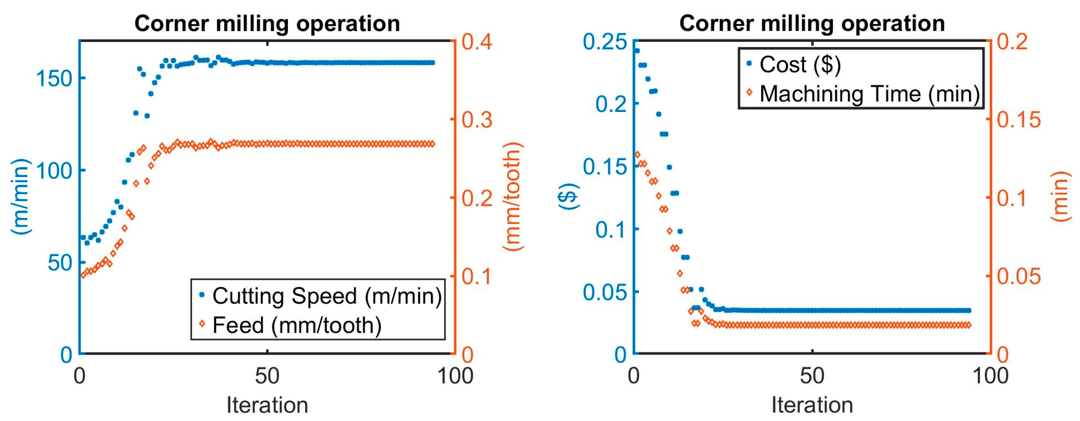
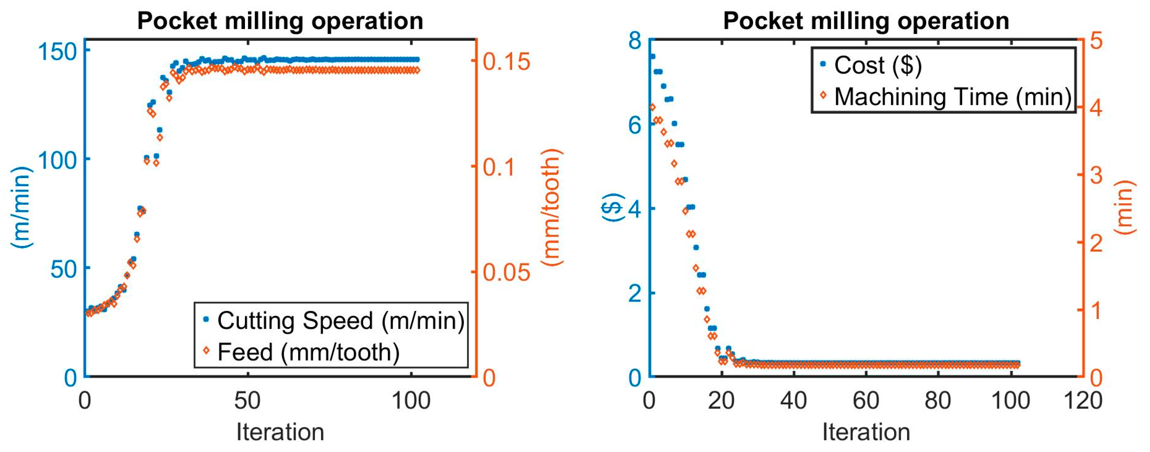
As shown in Figure 7, optimum machining parameters of the corner milling listed in

Table 6. Initial and optimum parameters of corner milling.

Initial Value		Output Value
Cutting Speed (m/min)	Feed (mm/tooth)	Cutting Speed (m/min)	Feed (mm/tooth)
60	0.1	157.85	0.268

were found at iteration 54, when the initial cutting speed and feed listed in Table 6 were used. Figure 8 shows the optimum machining parameters of the pocket milling parameters using the initial condition as listed in

Table 7. Initial and optimum parameters of pocket milling.

Initial Value		Output Value
Cutting Speed (m/min)	Feed (mm/tooth)	Cutting Speed (m/min)	Feed (mm/tooth)
30	0.03	145.57	0.145

.

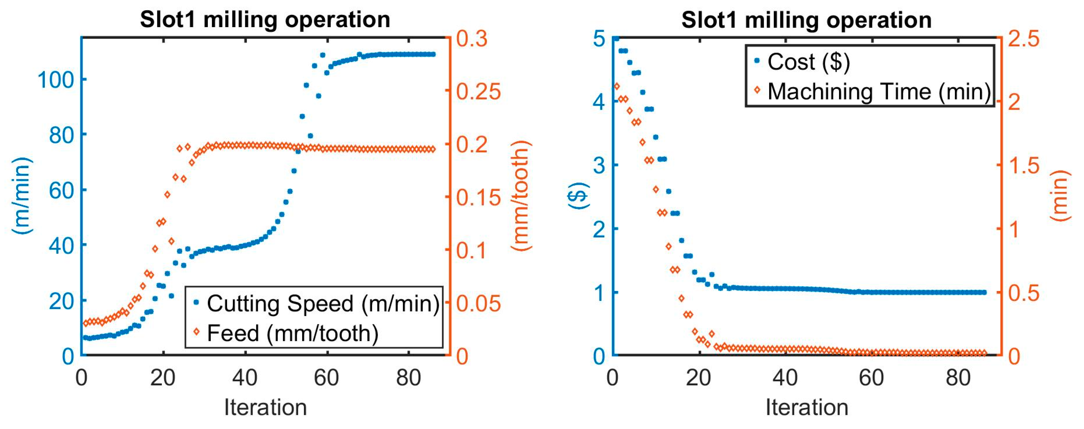
Figure 9 and Figure 10 show the optimum machining parameters of the slot1 milling and slot2 milling, whereas

Table 8. Initial and optimum parameters of slot1 milling.

Initial Value		Output Value
Cutting Speed (m/min)	Feed (mm/tooth)	Cutting Speed (m/min)	Feed (mm/tooth)
6	0.03	108.76	0.194

and

Table 9. Initial and optimum parameters of slot2 milling.

Initial Value		Output Value
Cutting Speed (m/min)	Feed (mm/tooth)	Cutting Speed (m/min)	Feed (mm/tooth)
6	0.03	111.78	0.378

list the optimized parameters with the initial cutting speed and feed. In general, we observed that the convergence of a solution is possible with less than sixty iterations.

4. Discussion

Table 10. Results by using optimum parameters.

Operation No	Operation Type	Tool No	Machining Cost ($)	Initial Cost ($)	Machining Time (min)	Tool Changing Time (min)	Setup Time (min)
1	Face	1	2.93	4.3	1.04	0.5	2
2	Corner	2	0.03		0.018	0.5	0
3	Pocket	2	0.31		0.164	0	0
4	Slot1	3	0.98		0.018	0.5	0
5	Slot2	3	0.04		0.021	0	0

summarizes the optimized machining cost and time for the operations used to produce the model part. Using the results in Table 10, we determined the final unit production time, unit cost, and profit as shown in

Table 11. Unit cost, time, and profit.

Unit Time (min)	Unit Cost ($)	Profit ($/min)
4.76	8.6	3.45

.

Constraint values of the maximum machine power are listed in Table 2. Power consumption for all machining operations should not exceed 8.5 kW to meet maximum machine power proposed by Tolouei and Bidhendi [7]. Constraint values of surface finish requirements are listed in Table 3, and surface finish requirements for all machining operations should be satisfied. Lastly, the cutting forces should not exceed the permitted cutting forces listed in Table 3. Optimized power consumption, surface finish, and cutting forces using Nelder–Mead methods are listed in

Table 12. Constraint values of optimum parameters.

Operation Type	Vo (m/min)	fo (mm/tooth)	Machining Power (kW)	Surface Finish (μm)	Cutting Force (kN)
Face milling	156.44	0.078	3.68	1.9	8.42
Corner milling	157.85	0.268	8.5	0.57	9.64
Pocket milling	145.57	0.145	8.5	0.17	10.4
Slot1 milling	108.76	0.194	8.47	0.25	13.96
Slot2 milling	111.78	0.378	8.48	0.95	13.61

. It should be noted that the optimum process parameters met specific constraint values by Tolouei and Bidhendi [7].

In this paper, the Nelder–Mead simplex method was used to find the maximum profit of milling operations by identifying optimum process parameters without violating any constraints. We compared the profit derived in this study with previous studies, as shown in

Table 13. Profit of each method.

Method	Profit ($/min)
Handbook Recommendation [7]	0.72
Tolouei and Bidhendi Feasible Direction [7]	2.64
Cuckoo Search [12]	2.82
PSO Algorithm [14]	2.88
Hybrid Differential Evolution [30]	2.82
Genetic Algorithm [13]	3.84
Modified Shuffled Frog-Leaping [15]	2.82
DATLBO Algorithm [16]	3.31
The Nelder–Mead Simplex Method	3.45

, and we found that the Nelder–Mead Method was able to produce a higher profit.

Even though the profit found by Abhishek [13], using the Genetic Algorithm, is higher than the Nelder–Mead simplex method, it should be noted that Abhishek arrived at an optimum feed of 0.264 (mm/tooth) for face milling. However, the surface finish requirement of 2 (μm) would limit the feed to be less than 0.079 (mm/tooth). Therefore, we arrived at a better solution while meeting the constraints and objective function suggested by Tolouei and Bidhendi. Finally, the Nelder–Mead simplex method not only improves production profit, but it will also increase productivity by eliminating unnecessary testing.

5. Conclusions

From the optimum parameters obtained by using the Nelder–Mead simplex method, the following can be concluded:

• Optimization methods that utilize the gradient of an objective function, which are composed of a non-linear system with constraint functions, have difficulty in arriving at an optimum solution efficiently.
• A profit improvement of 30% in the Nelder–Mead simplex method is observed when compared to Tolouei and Bidhendi feasible direction [7] because (a) it allows us to employ infeasible individuals efficiently, (b) the method is simple to utilize, and (c) it does not need parameter tuning.
• Even though overtravel was considered in this study, which was excluded from Tolouei and Bidhendi [7], a more profitable solution was found by using the Nelder–Mead simplex method while satisfying the suggested constraints.
• The Nelder–Mead simplex method used in optimizing the cutting parameters in CNC milling processes produced a better result than referenced studies.

In conclusion, when the Nelder–Mead simplex method was employed, the profit achieved was higher than the maximum profit obtained by Tolouei and Bidhendi [7]; this method is also more effective in predicting a solution. We expect that the Nelder–Mead simplex method will help industries achieve a higher profit in milling process optimization.

References

1. Stephenson, D.A.; Agapiou, J.S. Metal Cutting Theory and Practice; Dekker: New York, NY, USA, 2016; pp. 27–43. [Google Scholar]
2. Karandikar, J.; Kurfess, T. Cost optimization and experimental design in milling using surrogate models and value of information. J. Manuf. Syst. 2015, 37, 479–486. [Google Scholar] [CrossRef]
3. Li, J.; Lu, Y.; Zhao, H.; Li, P.; Yao, Y. Optimization of cutting parameters for energy saving. Int. J. Adv. Manuf. Technol. 2013, 70, 117–124. [Google Scholar] [CrossRef]
4. Chen, X.; Li, C.; Tang, Y.; Li, L.; Du, Y.; Li, L. Integrated optimization of cutting tool and cutting parameters in face milling for minimizing energy footprint and production time. Energy 2019, 175, 1021–1037. [Google Scholar] [CrossRef]
5. Faisal, N.; Kumar, K. Optimization of machine process parameters in EDM for EN 31 using evolutionary optimization techniques. Technologies 2018, 6, 54. [Google Scholar] [CrossRef] [Green Version]
6. Abbas, A.; Pimenov, D.; Erdakov, I.; Taha, M.; Soliman, M.; Rayes, M.E. ANN surface roughness optimization of AZ61 magnesium alloy finish turning: Minimum machining times at prime machining costs. Materials 2018, 11, 808. [Google Scholar] [CrossRef] [PubMed] [Green Version]
7. Tolouei-Rad, M.; Bidhendi, I. On the optimization of machining parameters for milling operations. Int. J. Mach. Tools Manuf. 1997, 37, 1–16. [Google Scholar] [CrossRef]
8. Iqbal, A.; Al-Ghamdi, K.A.; Hussain, G. Effects of tool life criterion on sustainability of milling. J. Clean. Prod. 2016, 139, 1105–1117. [Google Scholar] [CrossRef]
9. Anderberg, S.E.; Kara, S.; Beno, T. Impact of energy efficiency on computer numerically controlled machining. Proc. Inst. Mech. Eng. Part B J. Eng. Manuf. 2009, 224, 531–541. [Google Scholar] [CrossRef]
10. Kant, G.; Sangwan, K.S. Prediction and optimization of machining parameters for minimizing power consumption and surface roughness in machining. J. Clean. Prod. 2014, 83, 151–164. [Google Scholar] [CrossRef]
11. Wang, J. Multiple-objective optimisation of machining operations based on neural networks. Int. J. Adv. Manuf. Technol. 1993, 8, 235–243. [Google Scholar] [CrossRef]
12. Yildiz, A.R. Cuckoo search algorithm for the selection of optimal machining parameters in milling operations. Int. J. Adv. Manuf. Technol. 2012, 64, 55–61. [Google Scholar] [CrossRef]
13. Abhishek, A. Optimization of machining parameters for milling operations using a genetic algorithm approach. Int. J. Eng. Technol. Res. 2015, 3, 38–43. [Google Scholar]
14. Deepak, U. Optimization of milling operation using genetic and PSO algorithm. Bonfring Int. J. Softw. Eng. Soft Comput. 2011, 1, 8–14. [Google Scholar] [CrossRef] [Green Version]
15. Gomez, M.; Jurado, F. Machining parameters selection for milling operations using shuffled frog-leaping algorithm. Int. J. Emerg. Technol. Adv. Eng. 2015, 5, 50–59. [Google Scholar]
16. Zhai, Z.; Li, S.; Liu, Y. Parameter determination of milling process using a novel teaching-learning-based optimization algorithm. Math. Probl. Eng. 2015, 2015, 425689. [Google Scholar] [CrossRef]
17. Nelder, J.A.; Mead, R. A simplex method for function minimization. Comput. J. 1965, 7, 308–313. [Google Scholar] [CrossRef]
18. Kshirsagar, R.; Jones, S.; Lawrence, J.; Tabor, J. Optimization of TIG welding parameters using a hybrid nelder mead-evolutionary algorithms method. J. Manuf. Mater. Process. 2020, 4, 10. [Google Scholar] [CrossRef] [Green Version]
19. Tessema, B.; Yen, G. A self adaptive penalty function based algorithm for constrained optimization. In Proceedings of the IEEE International Conference on Evolutionary Computation, Vancouver, BC, Canada, 16–21 July 2006. [Google Scholar] [CrossRef]
20. Boothroyd, G.; Knight, W.A. Fundamentals of Machining and Machine Tools; CRC: Boca Raton, FL, USA, 2006; pp. 129–153. [Google Scholar]
21. Kronenberg, M. Machining Science and Application: Theory and Practice for Operation and Development of Machining Processes; Pergamon Press: Oxford, UK, 1966; pp. 99–143. [Google Scholar]
22. Rad, M.T. Studies on CAD/CAM Integration for Milling Operations Using Optimum Machining Parameters. Ph.D. Thesis, University of South Australia, Adelaide, Australia, 1997. [Google Scholar]
23. Singh, R.; Bajpai, V. Coolant and lubrication in machining. In Handbook of Manufacturing Engineering and Technology; Springer: London, UK, 2014; pp. 1–34. [Google Scholar] [CrossRef]
24. MDC. Machining Data Handbook, 3rd ed.; Machinability Data Center: Cincinnati, OH, USA, 1992; Volume 1, pp. 17–27. [Google Scholar]
25. Sahay, C.; Ghosh, S. Understanding Surface Quality: Beyond Average Roughness (Ra). Available online: https://peer.asee.org/understanding-surface-quality-beyond-average-roughness-ra (accessed on 2 July 2018).
26. Nguyen, T. Prediction and optimization of machining energy, surface roughness, and production rate in SKD61 milling. Measurement 2019, 136, 525–544. [Google Scholar] [CrossRef]
27. Bakerjian, R.; Mitchell, P. Tool and Manufacturing Engineers Handbook: A Reference Book for Manufacturing Engineers, Managers, and Technicians; Society of Manufacturing Engineers: Dearborn, MI, USA, 1993. [Google Scholar]
28. Subramanian, M.; Sakthivel, M.; Sooryaprakash, K.; Sudhakaran, R. Optimization of cutting parameters for cutting force in shoulder milling of Al7075-T6 using response surface methodology and genetic algorithm. Procedia Eng. 2013, 64, 690–700. [Google Scholar] [CrossRef] [Green Version]
29. Kaczmarek, J. Principles of Machining by Cutting, Abrasion and Erosion; Peter Peregrinus Limited: Stevenage, UK, 1976. [Google Scholar]
30. Yildiz, A.R. A new hybrid differential evolution algorithm for the selection of optimal machining parameters in milling operations. Appl. Soft Comput. 2013, 13, 1561–1566. [Google Scholar] [CrossRef]
Figure 1. Milling operations.
Jmmp 04 00066 g001
Figure 2. The Nelder–Mead simplex method process [18].
Jmmp 04 00066 g002
Figure 3. Flowchart for the Nelder–Mead optimization algorithm [18].
Jmmp 04 00066 g003
Figure 4. Case study drawing [7].
Jmmp 04 00066 g004
Figure 5. Plot showing profit, unit cost, and unit time for all operations examined in the case study assuming a constant feed of 0.8 mm/tooth.
Jmmp 04 00066 g005
Figure 6. Machining parameters (left) and results (right) for step operation of the case study.
Jmmp 04 00066 g006
Figure 7. Machining parameters (left) and results (right) for corner operation of the case study.
Jmmp 04 00066 g007
Figure 8. Machining parameters (left) and results (right) for the pocket operation of the case study.
Jmmp 04 00066 g008
Figure 9. Machining parameters (left) and results (right) for slot1 operation of the case study.
Jmmp 04 00066 g009
Figure 10. Machining parameters (left) and results (right) for slot2 operation of the case study.
Jmmp 04 00066 g010