Article

Evaluation of Prediction Accuracy for Anisotropic Yield Functions Using Cruciform Hole Expansion Test

1
Department of Mechanical Engineering, Daido University, 10-3 Takiharu-cho, Minami-ku, Naogoya 457-8530, Japan
2
JSOL Corporation, Tosabori Daibiru Building, 2-2-4 Tosabori, Nishi-ku, Osaka 550-0001, Japan
3
Chair of Metal Forming and Casting, Technical University of Munich, Walther-Meissner-Strasse 4, 85748 Garching, Germany
*
Author to whom correspondence should be addressed.
J. Manuf. Mater. Process. 2020, 4(2), 43; https://doi.org/10.3390/jmmp4020043
Submission received: 8 April 2020 / Revised: 28 April 2020 / Accepted: 29 April 2020 / Published: 3 May 2020

Abstract

:
To evaluate the prediction accuracy of the anisotropic yield function, we propose an original cruciform hole expansion test. Displacements on two axes were applied to the cruciform specimens with a hole in the center. The thickness strain in the region near the hole was compared to the simulation results. Because this forming test is free of friction and bending, it is an appropriate method to assess the anisotropic yield function without the influences of friction or the Bauschinger effect, or the need to consider the stress-strain curve in high-strain region. Hill1948, YLD2000-2D, and spline yield function which is an improved version of the Vegter model were selected, and 6000 series aluminum alloy sheets (A6116-T4) were used in this study. The parameter identification method of the spline yield function also proposed in this paper using the pseudo plane strain tensile test and optimization software. As a result, the spline yield function has better predictive accuracy than the conventional anisotropic yield functions Hill1948 and YLD2000-2D.

1. Introduction

High-tensile-strength steel sheets and aluminum alloy sheets are used for weight reduction of car bodies. Because of the difficulty in forming these materials, preliminary evaluations by numerical simulation are necessary. Hence, the requirements for the prediction accuracy of simulations of sheet metal forming are high, and further improvement is essential. An anisotropic yield function is indispensable for highly accurate simulation. Within this paper, we evaluate the prediction accuracy of anisotropic yield functions Hill1948 [1], YLD2000-2D [2], and the spline yield function [3].
To evaluate the prediction accuracy of the anisotropic yield function, a hole-expansion test has been carried out in many studies. For examples in [4,5,6,7], the thickness strain distributions along the hole edge and its surroundings were compared with the simulation results. This approach is convenient and effective for assessing the validity of anisotropic modeling, because the anisotropy of the material affects the thickness strain distribution near the edge of the hole. However, the results rarely agree well with the experimental results. It is difficult to validate anisotropic modeling by only considering the change in thickness distribution. In general, this hole-expansion test is relatively simple, but includes contacts between the material and the dies, as well as bending and back-bending deformation. Thus, it is necessary to consider not only the anisotropy of the material, but also friction, the stress-strain relation in the high-strain region, and the Bauschinger effect. However, it is not possible to separate these effects within the calculations. The Coulomb friction model is a simple and popular friction model; however, friction during the forming process is affected by surface pressure, sliding speed, and distance. There are friction models that consider these additional variables [8,9,10]; however, none take anisotropy into account. In [11], the influence of anisotropic hardening was investigated using a hole-expansion test. In addition to the anisotropic hardening, Suzuki et al. [12] considered the Bauschinger effect using the Yoshida-Uemori model [13] and the stress-strain curve in the high-strain region, which was obtained from a plane bending test using a biaxial tensile machine. However, because no advanced friction model was considered only qualitative comparisons could be conducted.
In this study, we calibrate and validate the spline yield function, and compare the results with those of other widely used yield functions for the sheet material A6116 aluminum alloy. To validate the yield function, biaxial tensile tests were conducted using cruciform specimens with a hole in the center. Because this forming test does not include friction and bending, it is possible to a quantitatively compare the experimental and simulation results.

2. Anisotropic Yield Functions

Several important anisotropic yield functions have been proposed. The input variables of these functions differ; hence, the types of material tests required also differ among functions. To minimize simulation costs, simple functions with relatively high precision are most desirable. However, for functions with high complexity, it is often desirable to increase the predictive accuracy, despite additional costs and material tests. The features of the important anisotropic yield functions are described below.
  • Hill 1948 [1]: this is the most popular anisotropic yield function especially in the car manufacturing industry because of its simplicity. For calibration of this yield function, the results of uniaxial tensile tests in three directions are required. Usually, parameters are identified from the flow stress in the rolling direction (RD) and Lankford coefficients (r-values) in three directions.
  • YLD2000-2D [2]: this is a widely used yield function and is implemented in the several commercial finite element (FE) simulation software tools. In the case of face-centered cubic lattice metal, such as aluminum alloy, it is recommended that the order is set to 8 [14]. To calibrate this yield function, the flow stresses and r-values at 0°, 45°, and 90° with respect to the RD, the equi-biaxial stress value, and the strain increment direction at the equi-biaxial stress state are used.
  • Vegter [15]: this yield function is defined in the principal stress space. In addition to the uniaxial tensile tests in five or more directions and a material test of the equi-biaxial stress state, plane-strain tensile tests are required in five or more directions. The Vegter model can consider the results of many material tests, but it requires substantial effort to determine all input variables, and it is difficult to conduct pure plane-strain tensile test.
Considering the feasibility of material testing and of industrial application, Hill 1948, YLD2000-2D, and the spline yield function, which is an improved version of the Vegter model and described in the next section, are compared in this paper.

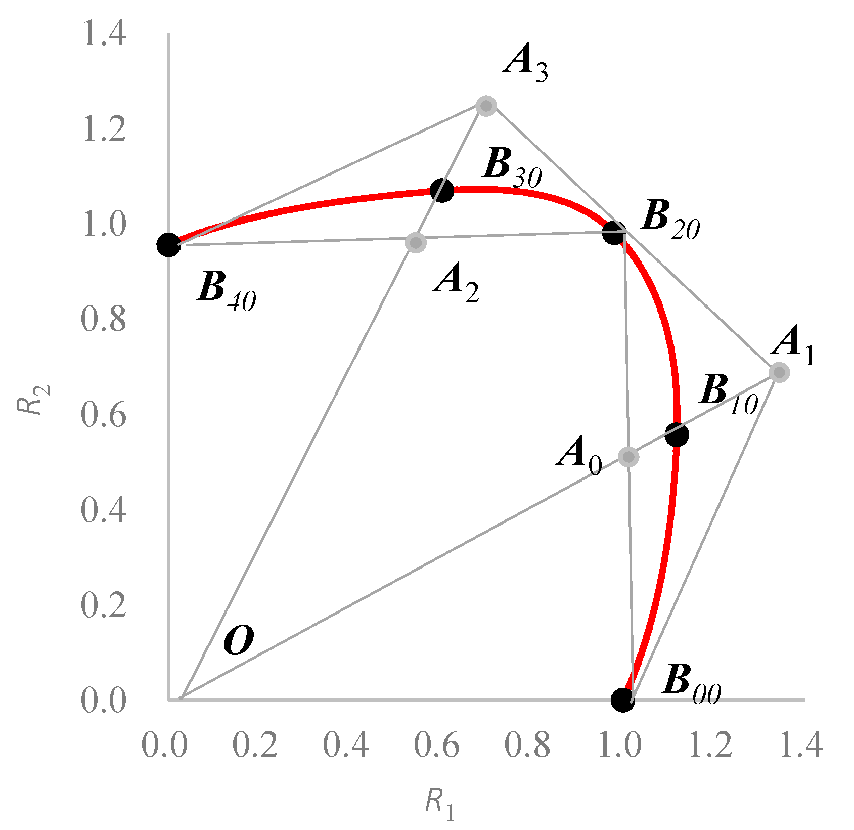
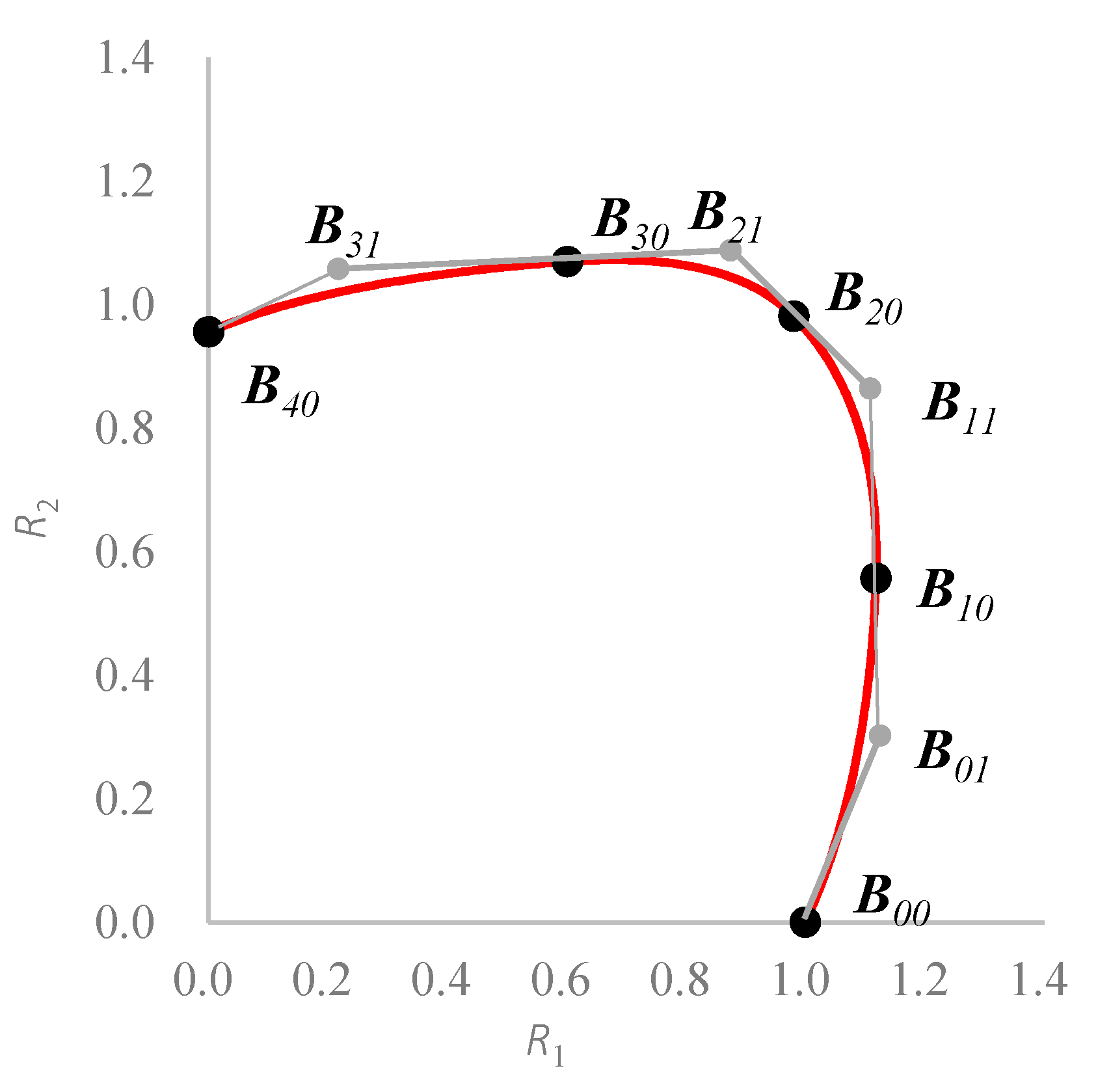
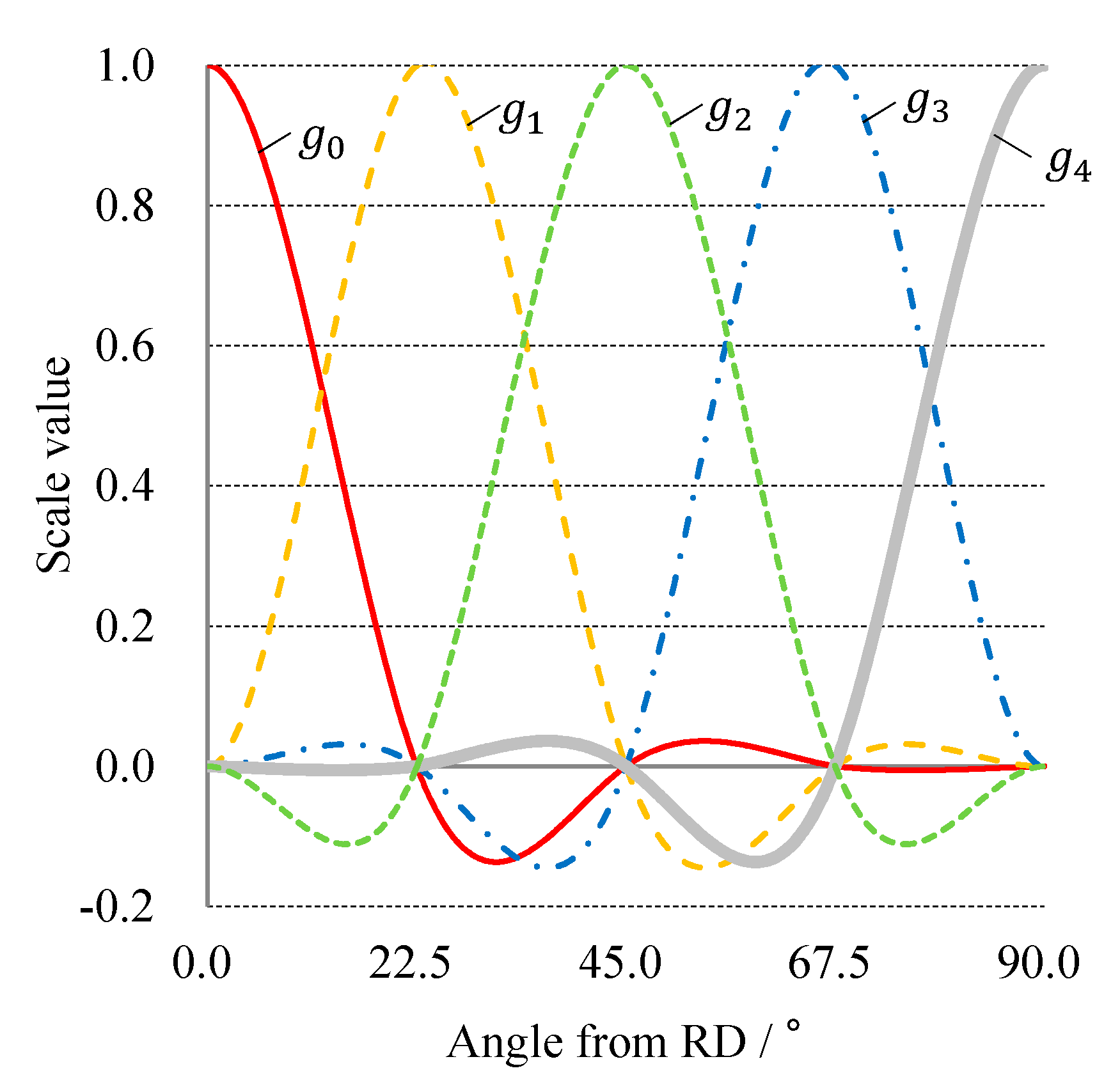
3. Spline Yield Function

The spline yield function is based on the Vegter model, and is defined in the principal stress space and enhanced by making its structure flexible. For interpolation function, spline functions are used instead of Fourier functions of the Vegter model. In previous studies [16,17], higher ordered or multi segmented yield loci than the Vegter model were used. The structure of a spline yield function is mathematically identical to a spline surface used in a computer aided design (CAD) system. In contrast with the Vegter model, the spline yield function does not require a pure plane strain stress state. This is one of its important advantages over the Vegter model. In the next section, we describe the calibration method of the spline yield function’s parameters using a pseudo plane strain tensile test and inverse analysis.
We consider the yield function with rotational symmetry with respect to the origin. We consider five points on the yield function, including the uniaxial stresses and the equi-biaxial stress in the first quadrant, as shown in Figure 1. This is a spline curve composed of four quadratic Bézier curve segments. B i 0 is the reference point on the curve ( i = 0 ,   1 ,   2 ,   3 ), B i 1 is the hinge point, and B i j is also the control point ( j = 0 ,   1 ). B i 1 is determined as an intersection of two tangent lines of B i 0   and B i j B 10 and B 30 do not need to be the exact plane-strain stress state. R ( u ) = ( R 1 , R 2 ) which is stress point on the normalized yield locus in the principal stress space of σ 1 and σ 2 is described as follows:
R ( u ) = ( 1 u ) 2 B i 0 + 2 ( 1 u ) u B i 1 + u 2 B ( i + 1 ) 0
where, u is the parameter of the Bézier curve ( 0     u     1 ). The direction of the principal stress, σ 1 and σ 2 are orthogonal to each other, and the smaller angle from RD is set to θ, and the other one is set to θ + 90°. To describe all the stress states, the angle θ between the direction of principal stress σ 1 and the RD must be continuously defined in the range of 0° to 90° in consideration of the symmetry condition due to the orthotropic anisotropy. In this study, five directions of σ 1 are defined discretely at 22.5° intervals, and R ( θ , u ) is defined continuously by interpolation using a spline basis function as follow:
R ( θ , u ) = k = 0 4 g k ( θ ) R k ( u )         ( k = 0 ,   1 ,   2 ,   3 ,   4 )
where R k ( u ) means the “k”th R ( u ) , if k = 1, the angle of σ 1 respect to the rolling direction is 22.5°. g k ( θ ) is a one-dimensional cubic spline basis function and is given by the following boundary conditions ( l = 0 ,   1 ,   2 ,   3 , 4 ).
g k ( l 4 · 90 ° ) = δ k l
g k θ | θ = 0 ° = g k θ | θ = 90 ° = 0
g k ( θ ) is drawn in Figure 2.
The convexity condition of the yield function and a relationship between the principal stress and the stress components in the global coordinate system is described in the Appendix A. B 00 , B 20 , and B 40 and their normal vectors determined from the uniaxial tensile tests and bulge test, and the parameters pk and qk were introduced to identify B 10 , B 30 and their normal vectors in Figure 1.
In Figure 3, A 1 is the intersection point of the tangent lines at B 00 and B 20 , A 0 is the intersection point of the lines from O to A 1 and B 00 to B 20 . The parameters p0, p4 and q0, q4 are defined as follows:
B 10 = ( 1 p 0 ) A 0 + p 0 A 1
B 30 = ( 1 p 4 ) A 2 + p 4 A 3
n 10 = ( 1 q 0 ) n 00 + q 0 n 20 | ( 1 q 0 ) n 00 + q 0 n 20 |
n 30 = ( 1 q 4 ) n 40 + q 4 n 20 | ( 1 q 4 ) n 40 + q 4 n 20 |
where, n i 0 is the normal vector at B i 0 . In Figure 3, R 1 is in the RD and R 2 is 90° to the RD. The parameters p1, p3, q1, and q3, as well as p0, p4, q0 and q4 are determined for R 1 at 22.5° to the RD and R 2 at 112.5° to the RD which is the same as at 67.5° to the RD because of symmetry. The parameters p2 and q2 are also determined for R 1 at 45° to the RD in the same way. The spline yield function was implemented using a user subroutine of LS-DYNA, which is a commercial code with dynamic explicit method. These parameters are identified by inverse analysis described in the next section.

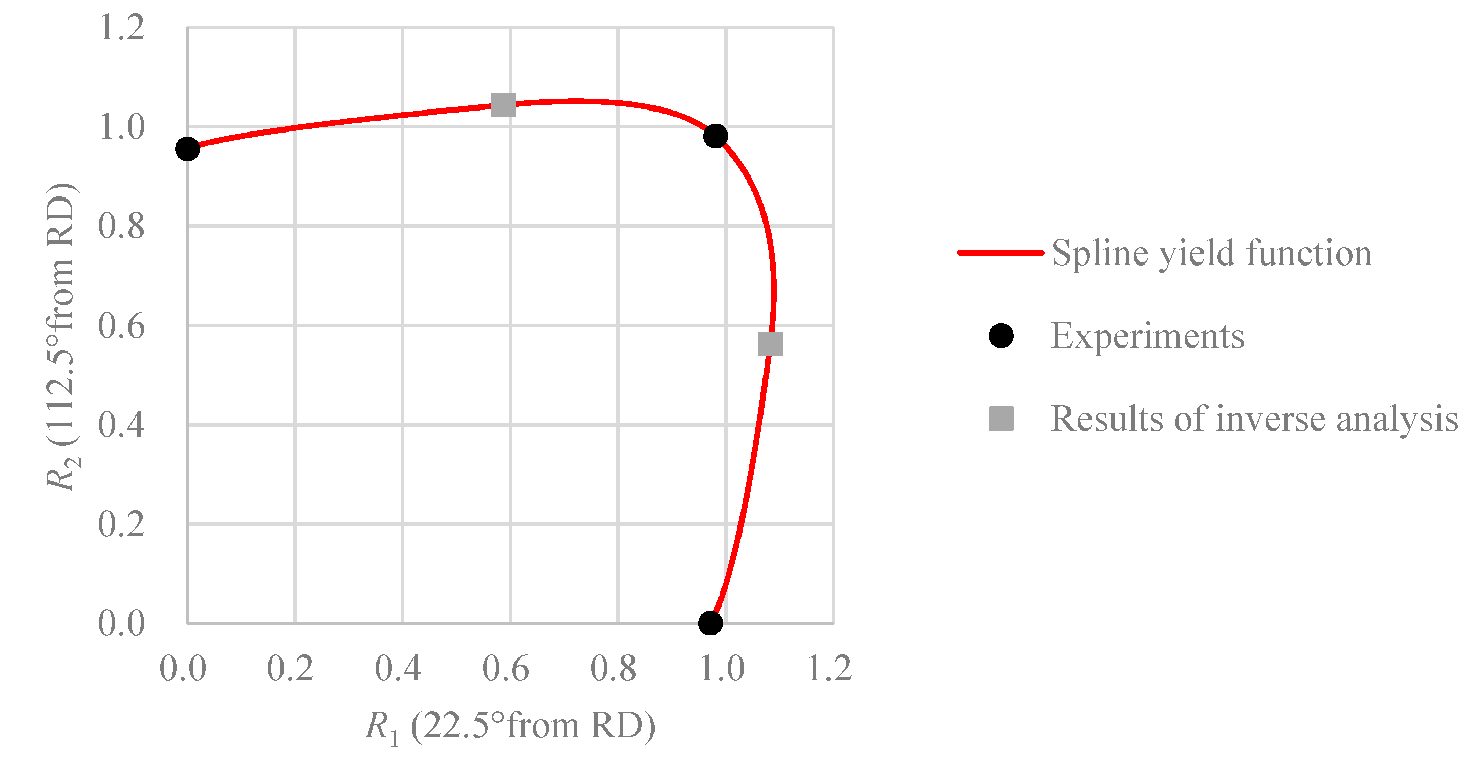
4. Calibration of Spline Yield Function

To identify the material parameters for three yield functions, three different types of material experiments were carried out. The thickness of the A6116 specimen was 0.93 mm and T4 solution heat treatment was conducted. The specimens for the uniaxial tensile tests and the pseudo plane-strain tensile tests were processed by wire cutting.

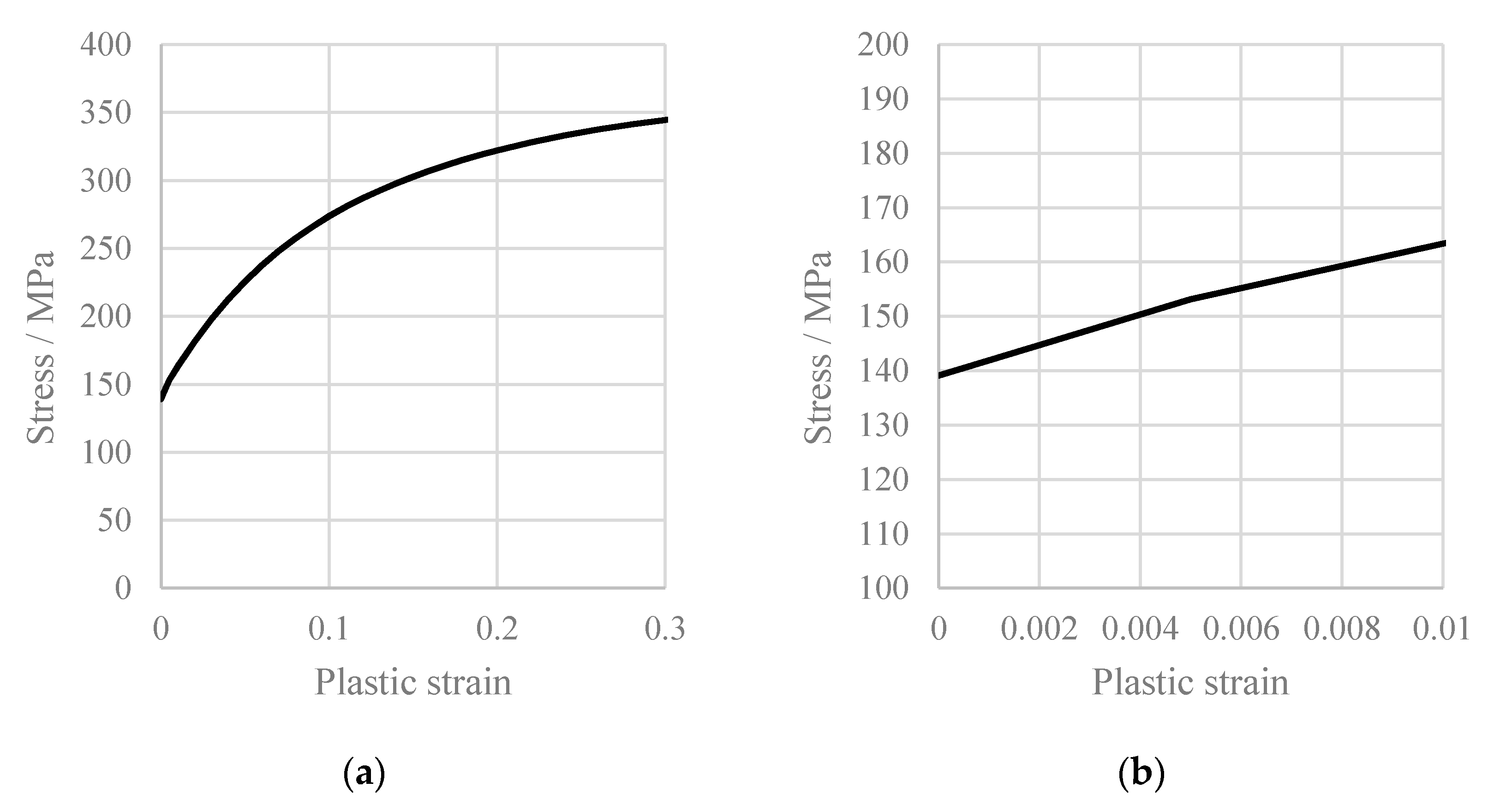
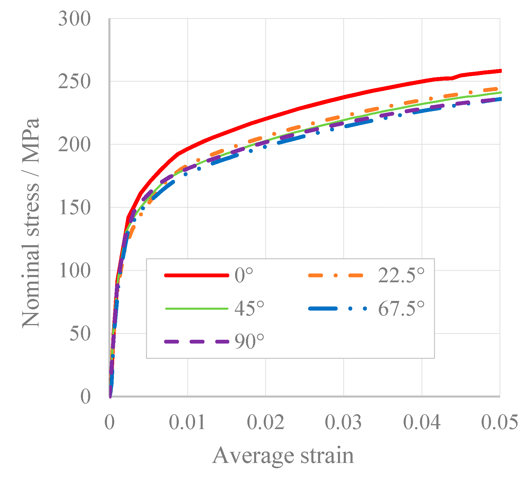
4.1. Uniaxial Tensile Tests

Uniaxial tensile tests are conducted for 5 specimens with tensile directions of 0°, 22.5°, 45°, 67.5° and 90° from the RD. Three valid repetitions were carried out for each experiment. The material properties obtained from these tests are summarized in Table 1. The normalized stress was determined when the plastic work in each direction was equal to the reference plastic work in the 0° tensile direction. The effective plastic strain was set to 0.05. The stress-strain curve in the 0° direction, which was extended from 0.2 by the Voce approximation, is shown in Figure 4. The anisotropy of the sheet metal is characterized by r-value, and the distribution of the anisotropic behavior of the material can be seen in Figure 5. Within this study, the r-value was calculated as width plastic strain divided by thickness plastic strain, the r ˜ -value was defined as the ratio of the width plastic strain increment to the plastic thickness strain increment. An accurate calculation was undertaken for the tangential direction of the equi-plastic work surface in the uniaxial stress state by using the r ˜ -values.

4.2. Bulge Tests

To measure the equi-biaxial stress and its strain increment ratio corresponding to the plastic strain of the uniaxial tensile test, hydraulic bulge tests were conducted. The diameter of the die was 123 mm. Three repetitions were carried out for each of experiment. The digital image correlation (DIC) system GOM ARAMIS was used to measure the curvature radius, ρ , and the strain, ε x or ε y , at the apex of the bulge specimen. The equi-biaxial stress state at the apex of the specimen was assumed to be σ b = σ x = σ y . For the determination of σ b , the following equation was used.
σ b = p ρ 2 t
where p is the oil pressure during the bulge test, and t is the sheet thickness at the apex of the specimen, which is calculated assuming constant volume during plastic deformation, and using the strain, ε x and ε y . In Table 2, the normalized stress and strain increment ratio are shown for a reference effective plastic strain of 0.05.

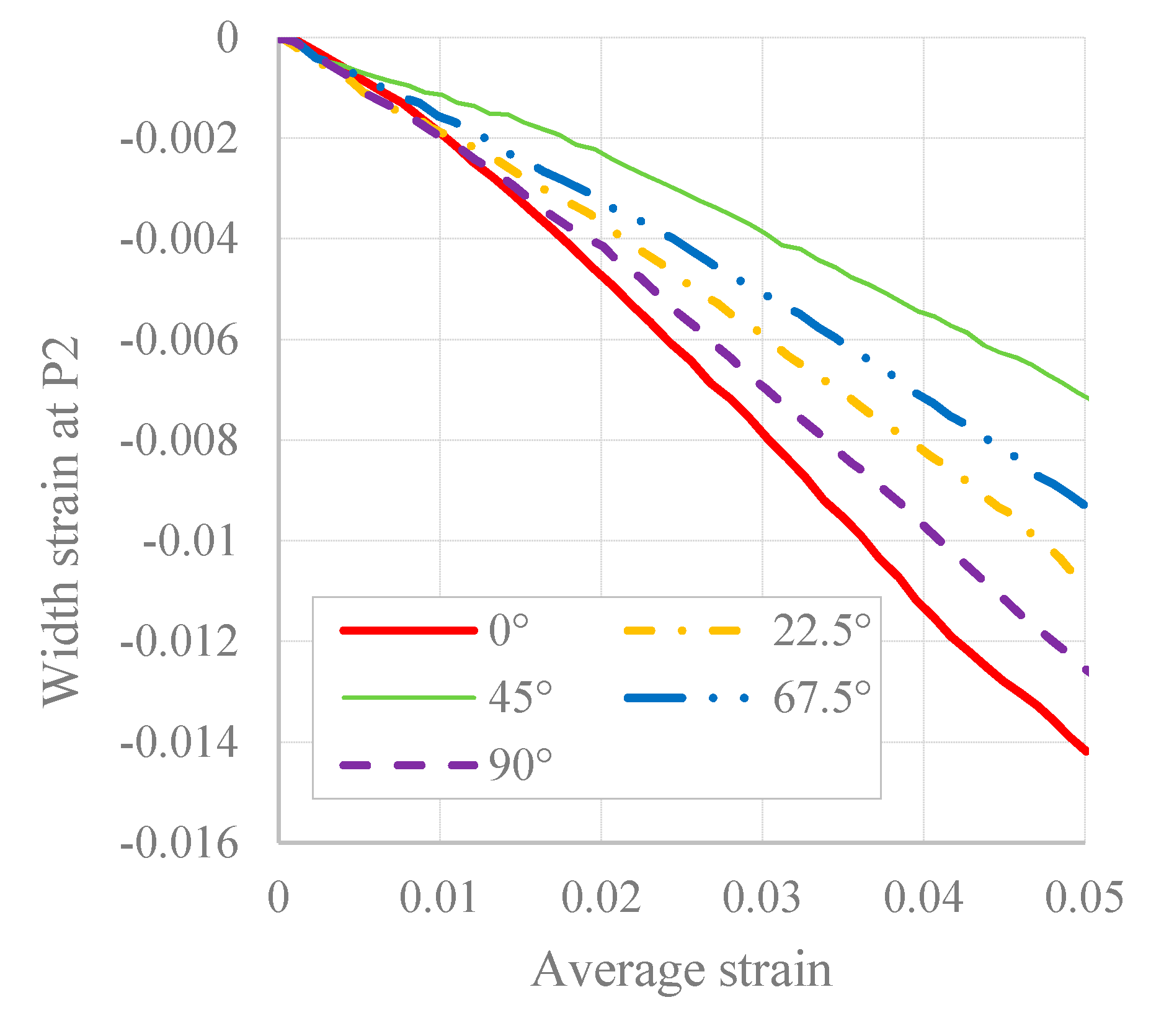
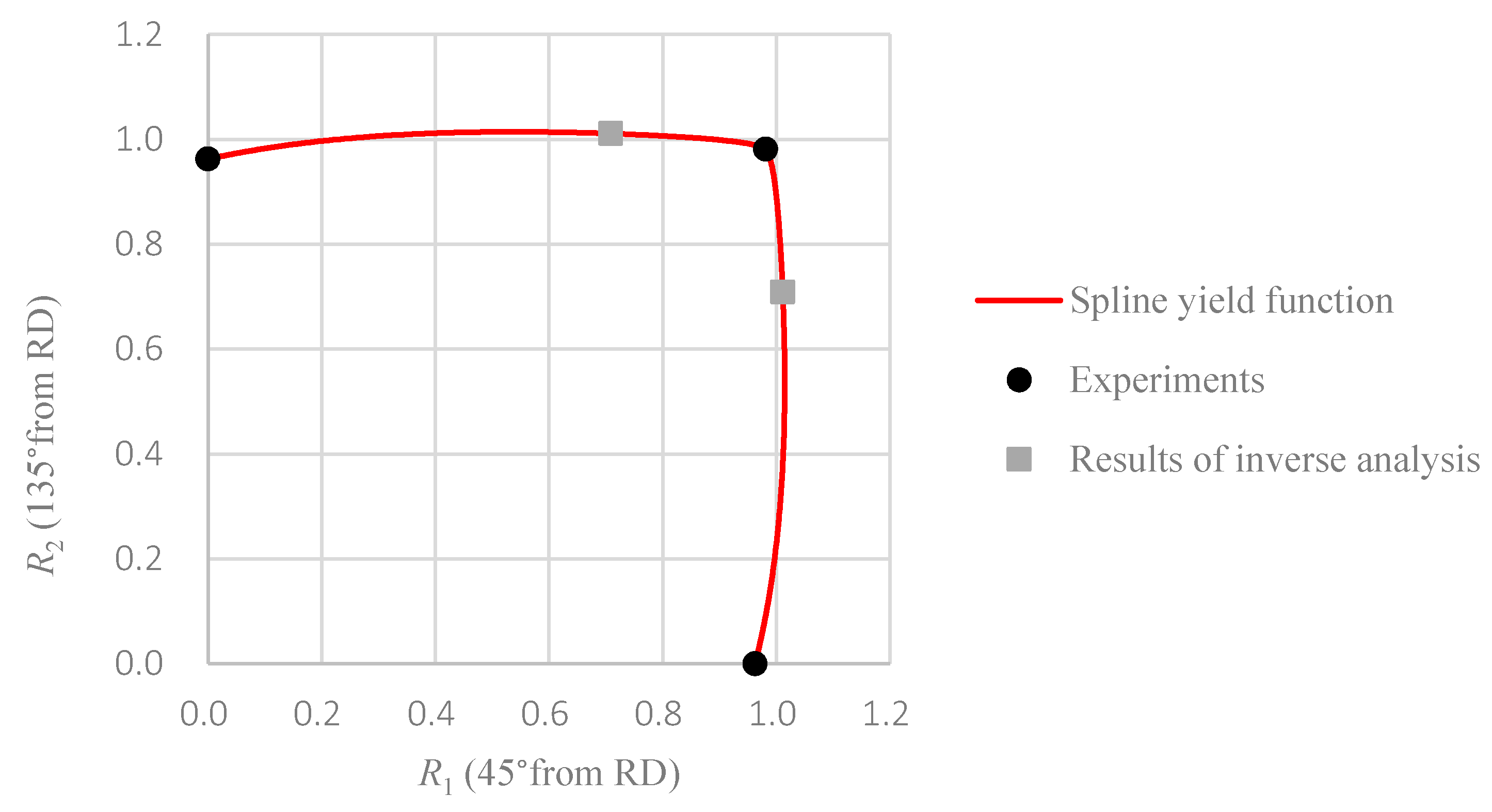
4.3. Pseudo Plane Strain Tensile Tests

Pseudo plane-strain tensile tests were carried out to determine the parameters for the spline yield function, which are described in Section 4.4. The specimen geometry, which is shown in Figure 6, with a width of 30 mm and length of 60 mm allows the same clamping system to be used for the uniaxial tensile tests. This geometry creates an approximately plan-strain stress state in the center of specimen; however, the strain is not homogenous over the width of the specimen. Similar to the uniaxial tensile test, three valid repetitions in the five tensile directions were carried out, and the load and strain were measured. ARAMIS was used to measure the strain at the center point, P 1 , of the specimen and the position P 2 , which is 5 mm in the tensile direction from the center (Figure 7). Figure 7 shows the maximum principal strain distribution of the specimen at 0° to RD. In order to compare with the simulation results later, the average strain was introduced as an axial representative strain. The average strain, ε a , was defined as ε a = { ε x ( P 1 ) + 2 ε x ( P 2 ) } / 3 , where the tensile direction is x and the specimen width direction is y. Post processing parameters of DIC are used 0.2 mm as distance of points, 10 mm as facet size. Figure 8 shows the relationship between the nominal stress and the average strain, and Figure 9 shows the relationship between the strain in the width direction at P 2 and the average strain. These results were applied for inverse analysis using the FE analysis software LS-DYNA.
Inverse analysis using FE simulation was applied to determine pk and qk from the results of the pseudo plane strain tensile test. The optimization software LS-OPT was used for this inverse analysis, and a mean square error method was adopted, which had two variables and two objective functions. The input variables were pk and qk and a relationship between a tensile force and the average strain (defined in Section 3) was used for one of the objective functions. The other objective function was the relationship between the strain at P2 in the width direction and the average strain. A FE model for the pseudo plane strain tensile test was determined, as shown in Figure 10. The mesh size was investigated as far as necessary strain, which maximum average strain is 5.0%. The 1 mm mesh size and 0.5 mm mesh size were compared, and the difference of the load force was less than 3% when the average strain was 5.0%. The 1mm mesh was adopted in consideration of simulation cost. The solutions of this optimization, which are parameters of spline yield function, are shown in Table 3. Furthermore, comparisons of the experimental results in 0° direction and the results of the FE simulation after an optimization of the objective functions are shown in Figure 11.
The following conditions are fully satisfied in the spline yield function: The flow stresses and r-values in 5 directions; the equi-biaxial stress and its strain increment direction; and the stresses near the plane strain in the five directions and their normal vectors. By contrast, the Vegter model could not be used, because this requires the pure plane-strain tensile test, so it is difficult to determine in the same material test.

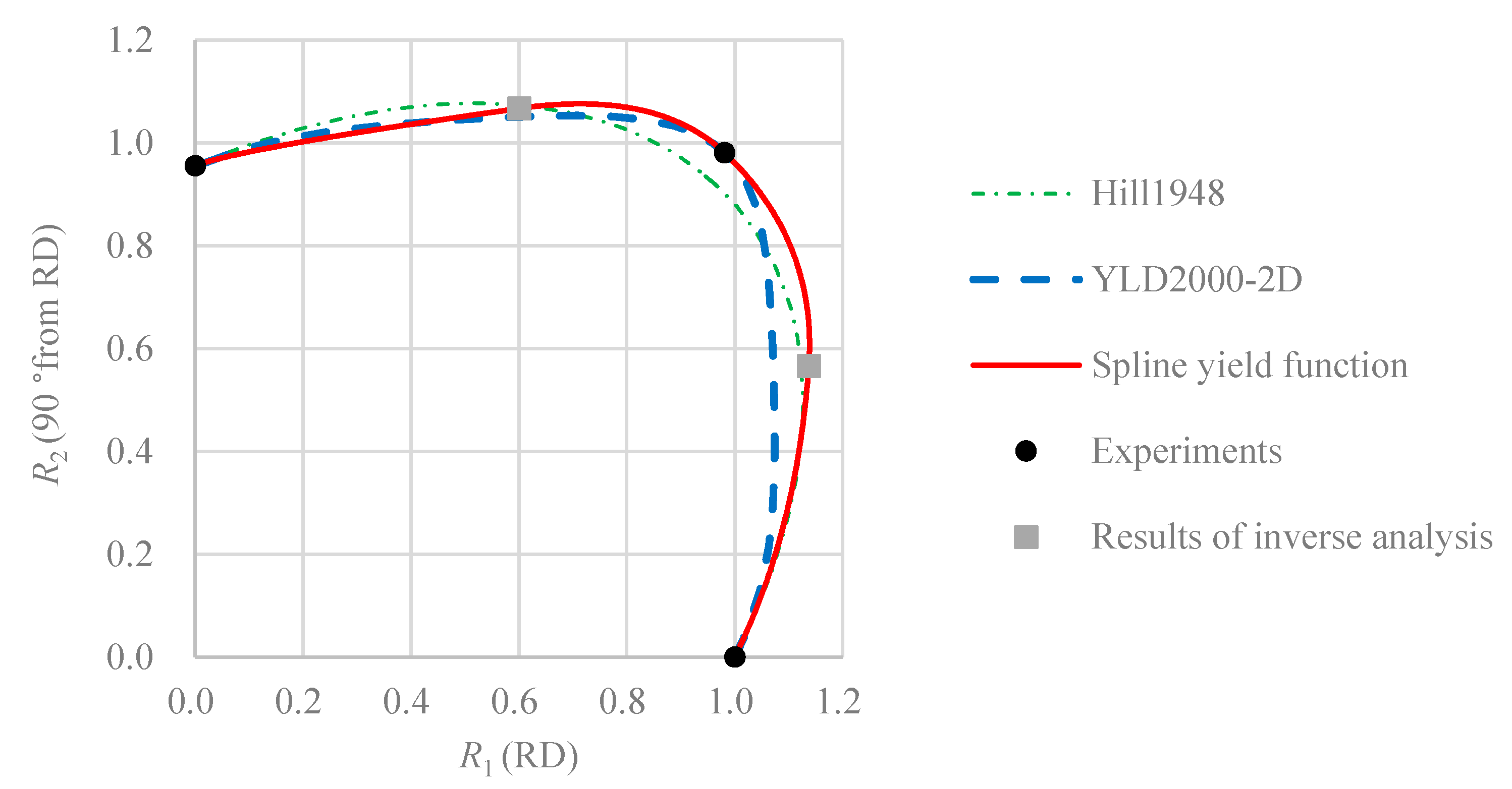
4.4. Comparison of the Equi-Plastic Work Surface Shape

The normalized equi-plastic work surfaces of the three yield functions, identified by aforementioned material tests, are shown in Figure 12, Figure 13 and Figure 14. Figure 12 also shows the results obtain using Hill 1948 and YLD2000-2D for comparison. A description of the parameter identification is given in the next section. The horizontal axis of Figure 12 corresponds to the RD and the vertical axis is 90° from the RD. The horizontal axis of Figure 13 is 22.5° with respect to the RD and the vertical axis is 112.5° (equal to 67.5° because of symmetry). The horizontal axis of Figure 14 is 45°, the vertical axis is 135° (equal to 45° because of symmetry). In Figure 13 and Figure 14, only the spline yield function is shown. because other yield functions are difficult to show in the principal stress space except when the horizontal axis is the RD. The above-mentioned equi-plastic work surfaces were normalized with respect to the plastic work of the uniaxial tensile test for the 0° tensile direction. The reference plastic strain was 0.05. Depending on angle of the axis in the principal stress space, the shape of spline yield function changes substantially for this material.

5. Evaluation of Anisotropic Yield Functions
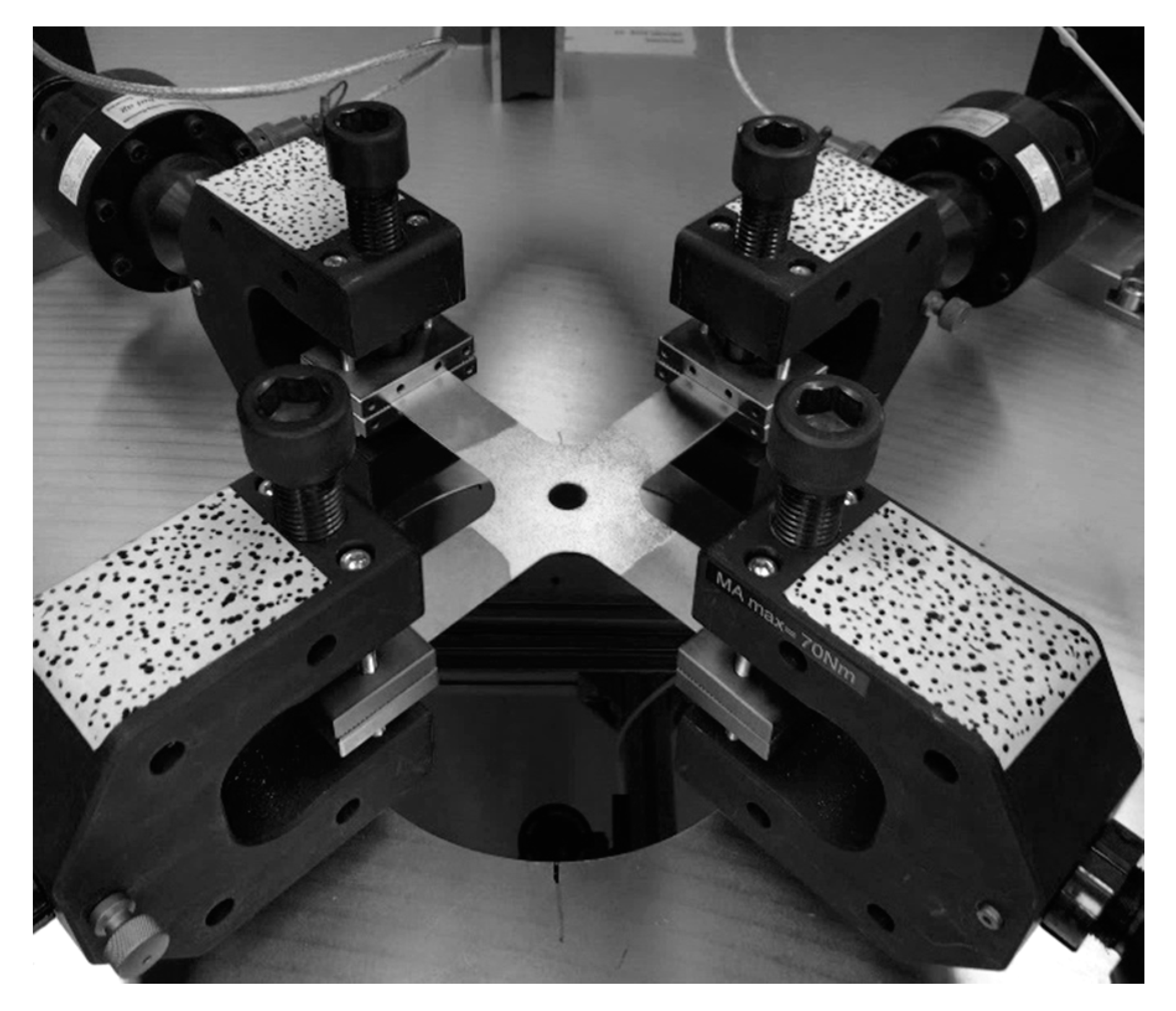
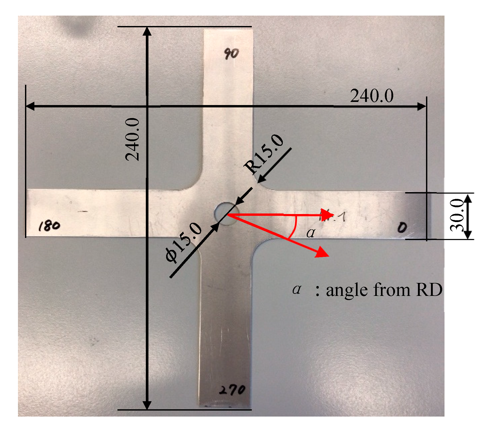
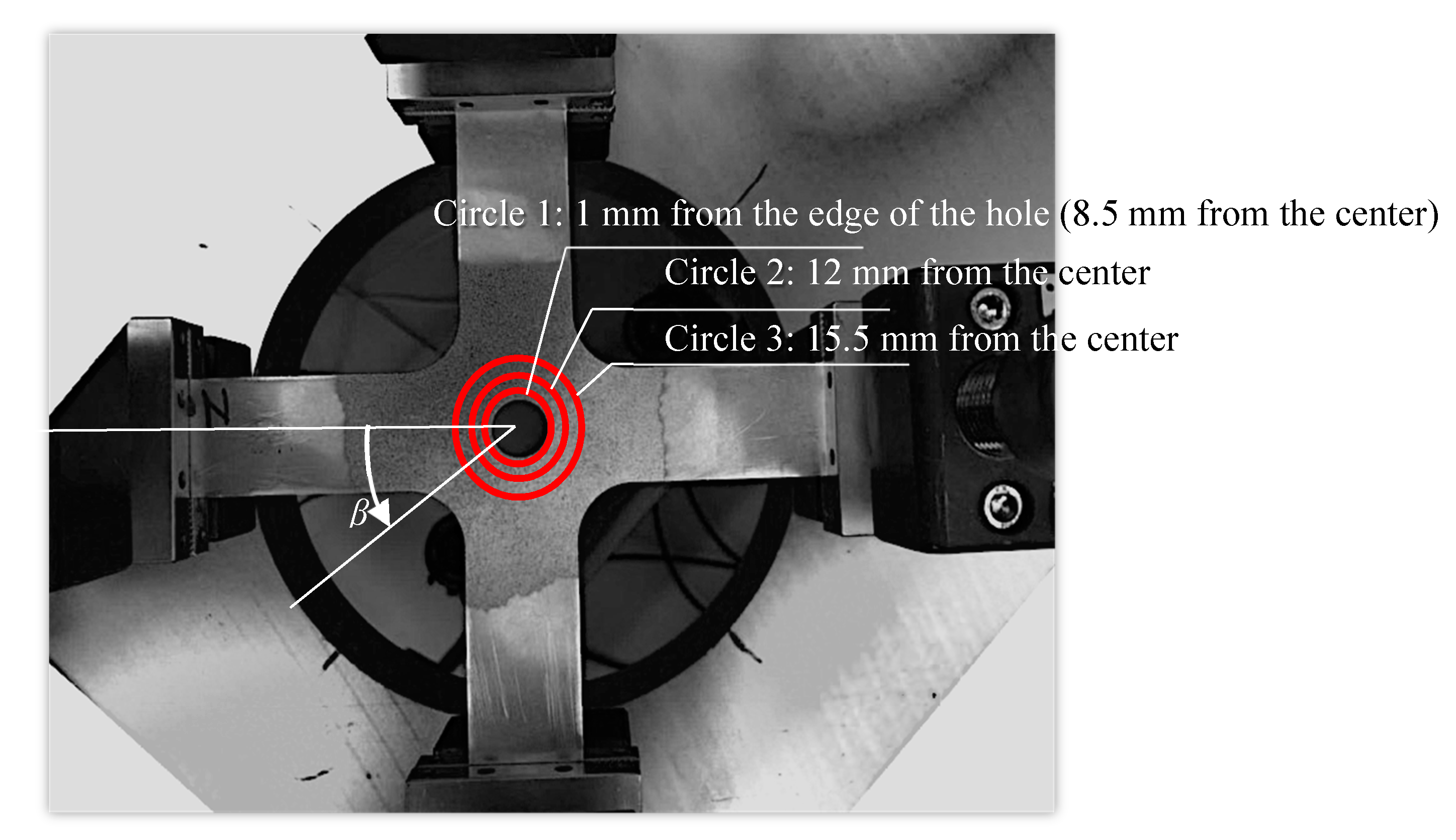
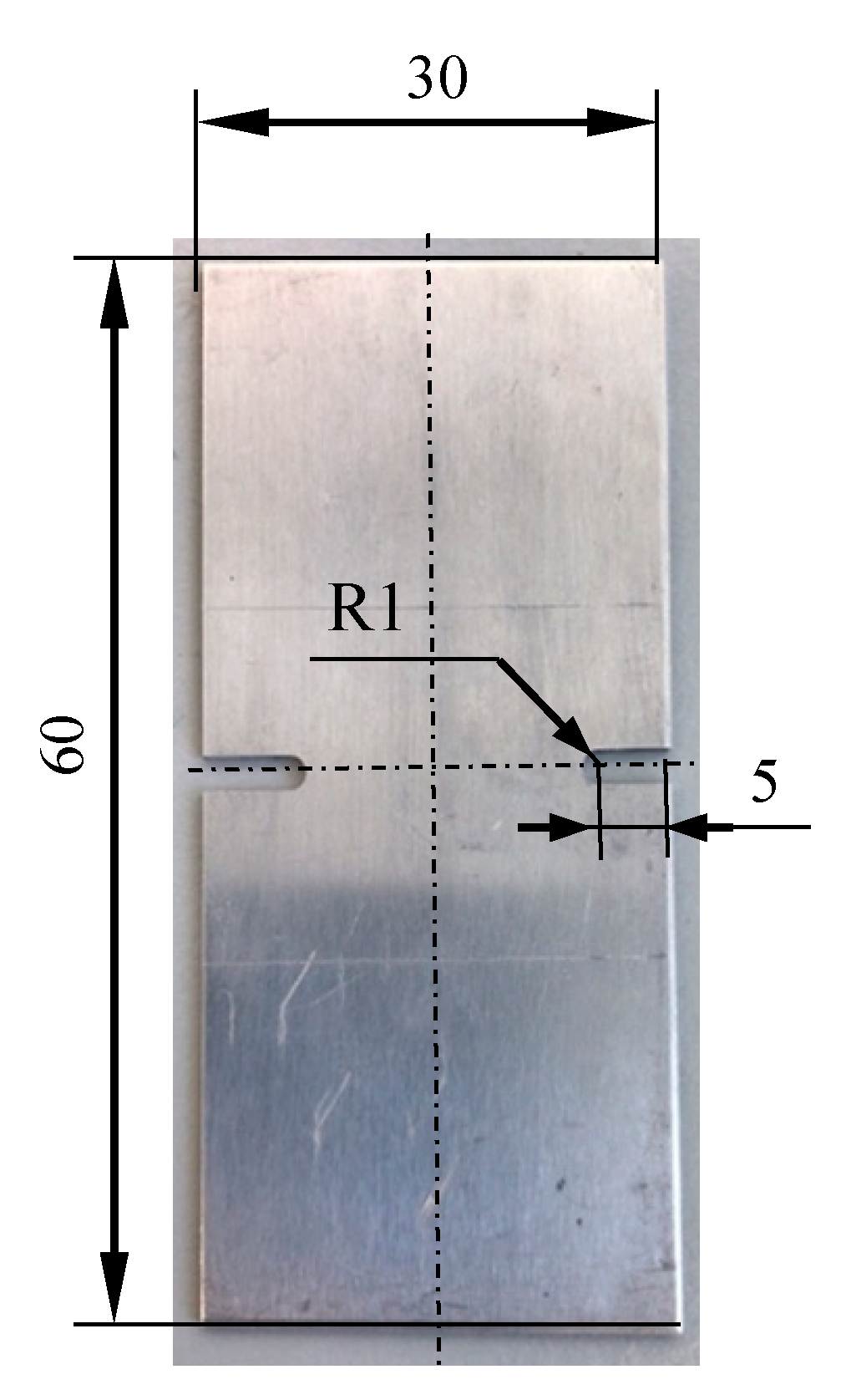
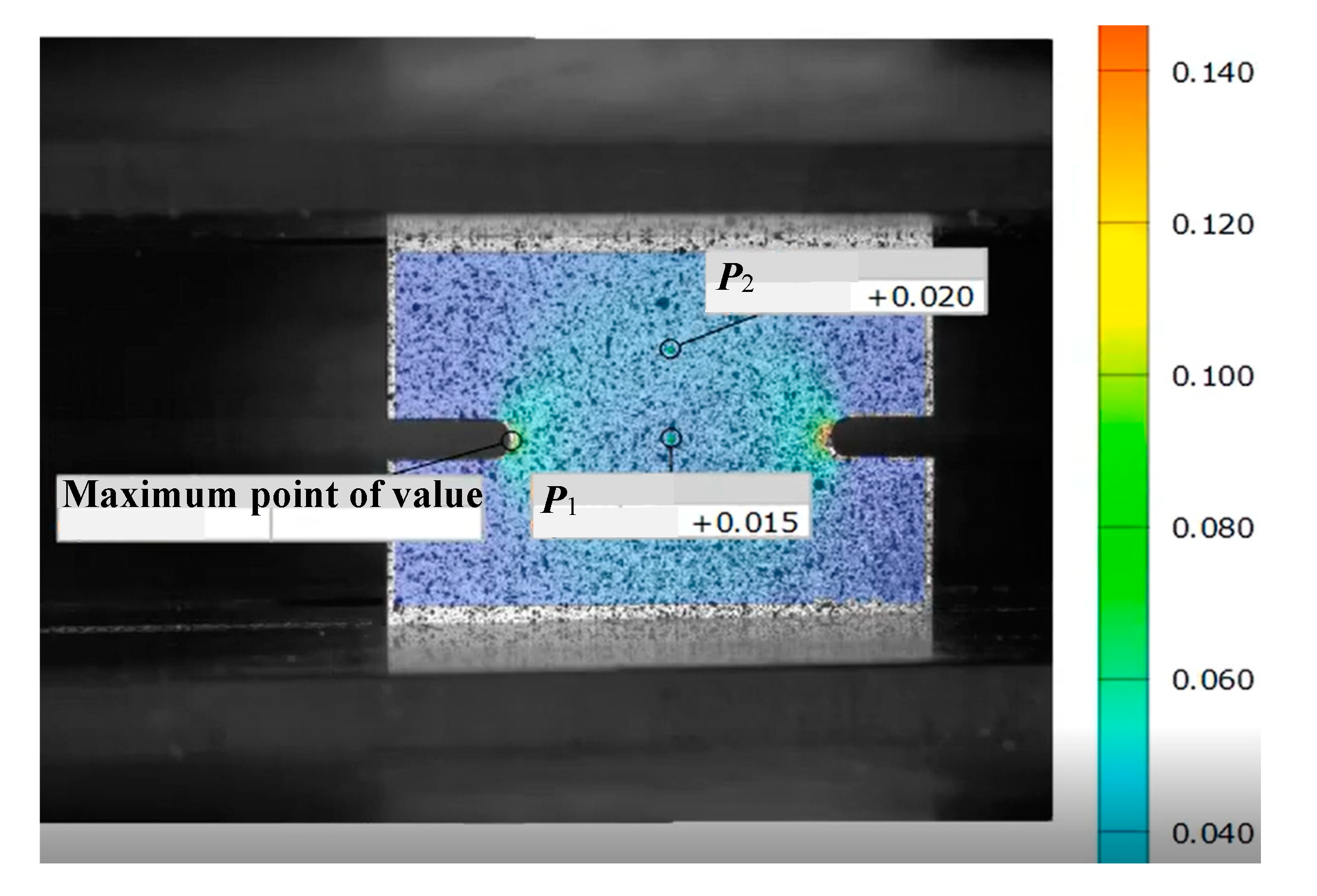
5.1. Experiment

To evaluate the prediction accuracy of the spline yield function, we carried out in-plane cruciform tests, which are free of friction and bending using the biaxial tensile test machine [18], as shown in Figure 15. The cylinders of both axes can be controlled by load or displacement. The strain was measured by the LIMESS DIC system, using four cameras installed above the specimen. The cruciform specimens were manufactured by milling and the face of the cross section was fine-grained. To allow the best comparison of experimental and simulation data, the tests were carried out by displacement control because the displacement can be directly used as a boundary condition in the simulation model.
In total, six sets of experiments with three values of α and two displacement ratios were conducted (Table 4). Thereby, the angle between the horizontal arm of the specimen and the RD is α (Figure 16). Three valid repetitions were carried out. For a displacement ratio of 2:1, velocities of 4 and 2 mm min−1 were used. For the ratio 1:1, the velocity was set to 2 mm min−1 in both axes. The frequency of DIC system was 5 frames s−1. The maximum and minimum principal true strain were determined using the software istra4D along the specified circle, Subsequently, the thickness strain was calculated assuming constant volume during plastic deformation. Post processing parameters of DIC are used 0.1 mm as distance of points, 10 mm as facet size.

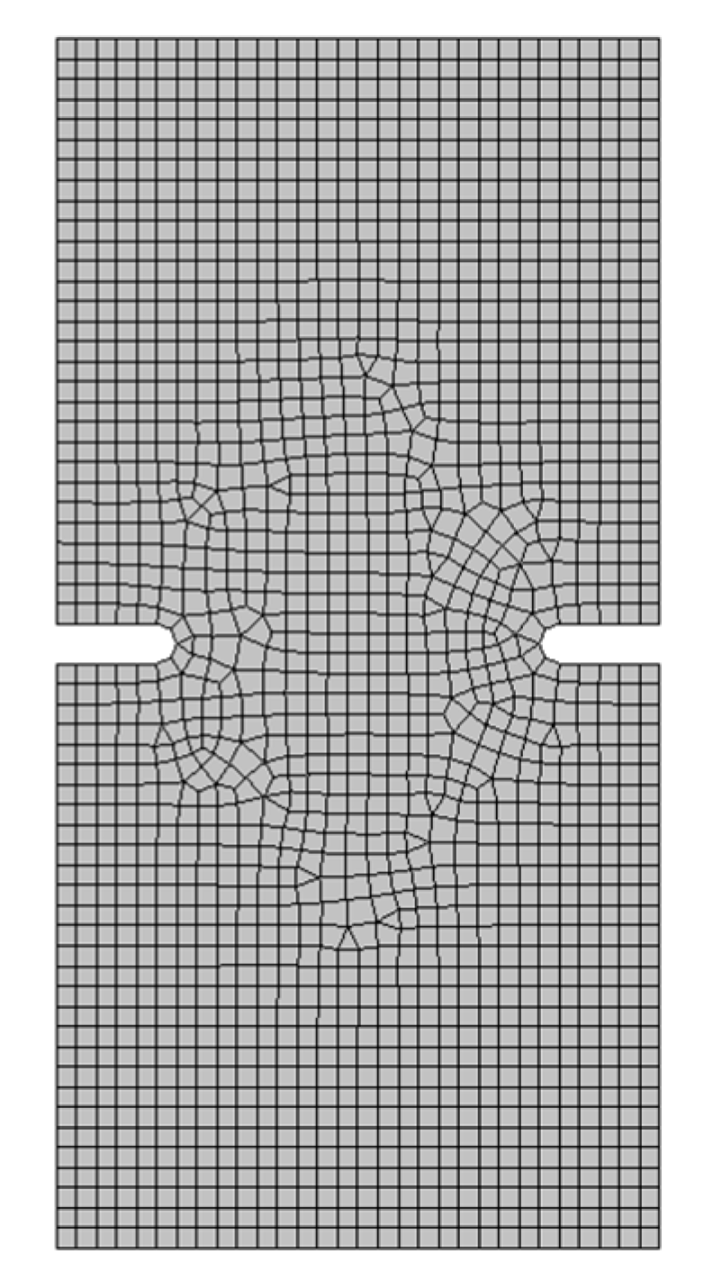
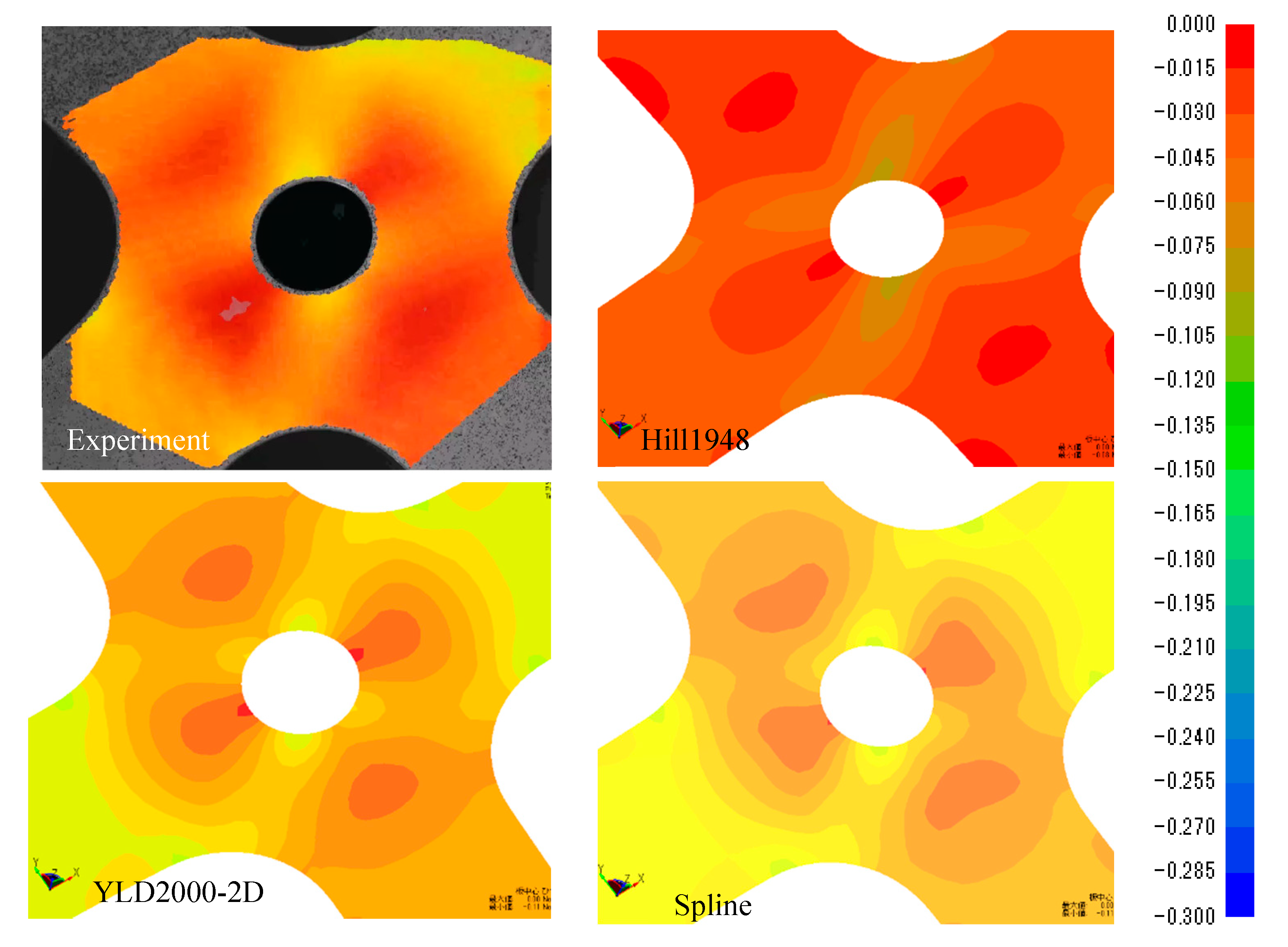
5.2. Numerical Analysis

LS-DYNA was used for this FE analysis. In FE model, a fine mesh size of less than 1 mm was used along the center hole. The displacement constraints were given as boundary condition, and the assumed strain shell elements [19] were used. To determine the anisotropic parameters for Hill1948 yield function, three r-values at 0°, 45°, and 90° direction relative to the RD in Table 1 were used. The order m of YLD2000-2D was set to 8, the anisotropic parameters α1 to α8 [2] were numerically determined using the following experimental results: the flow stresses and the r-values at 0°, 45°, 90°, equi-biaxial stress and strain increment ratio rb in Table 2. Anisotropic parameters α1 to α8 and m are shown in Table 5.

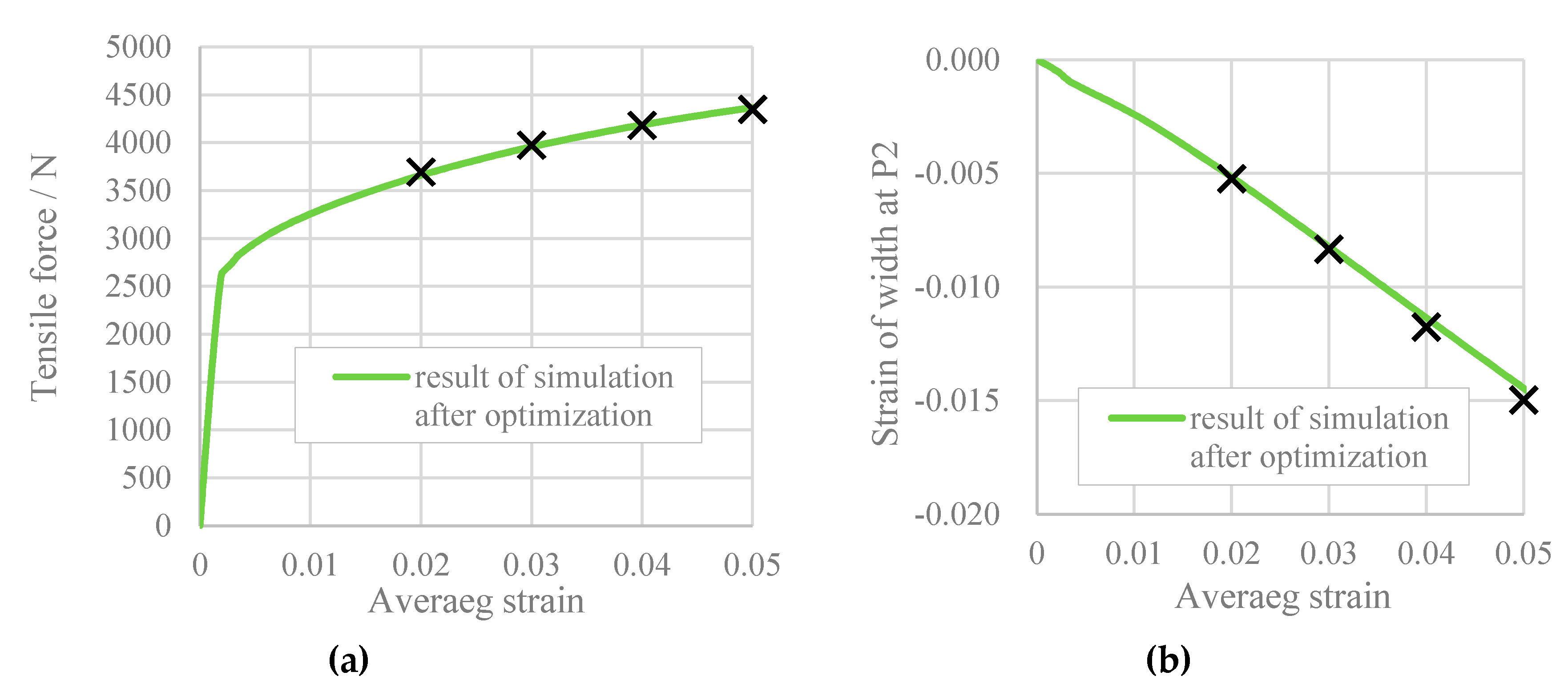
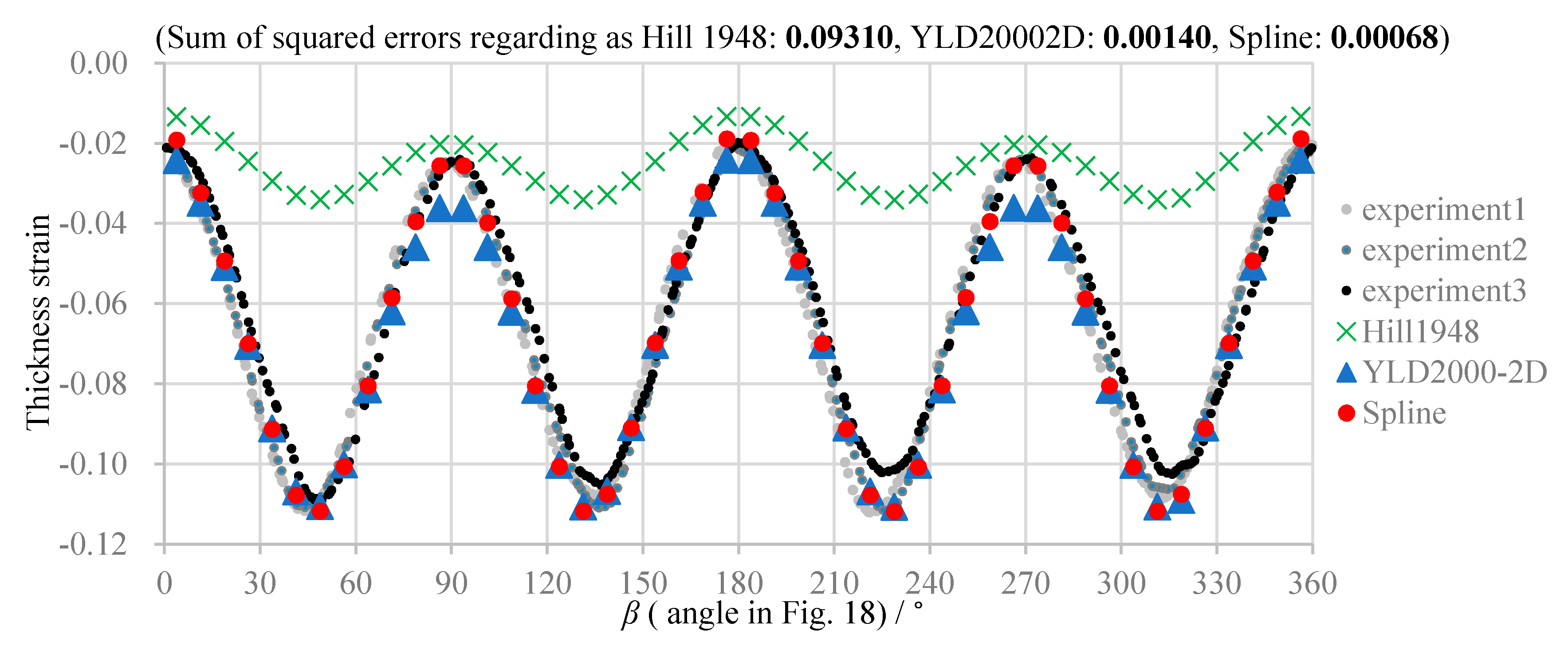
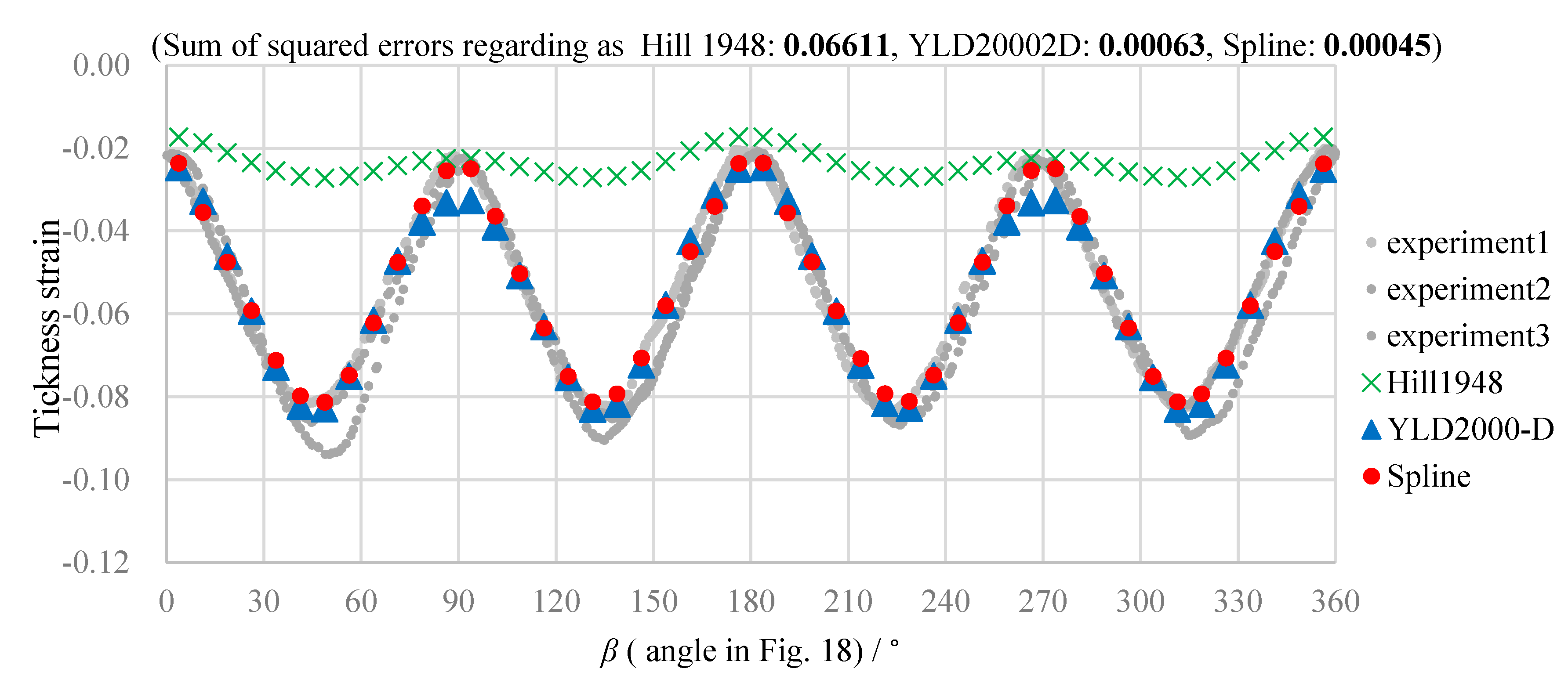
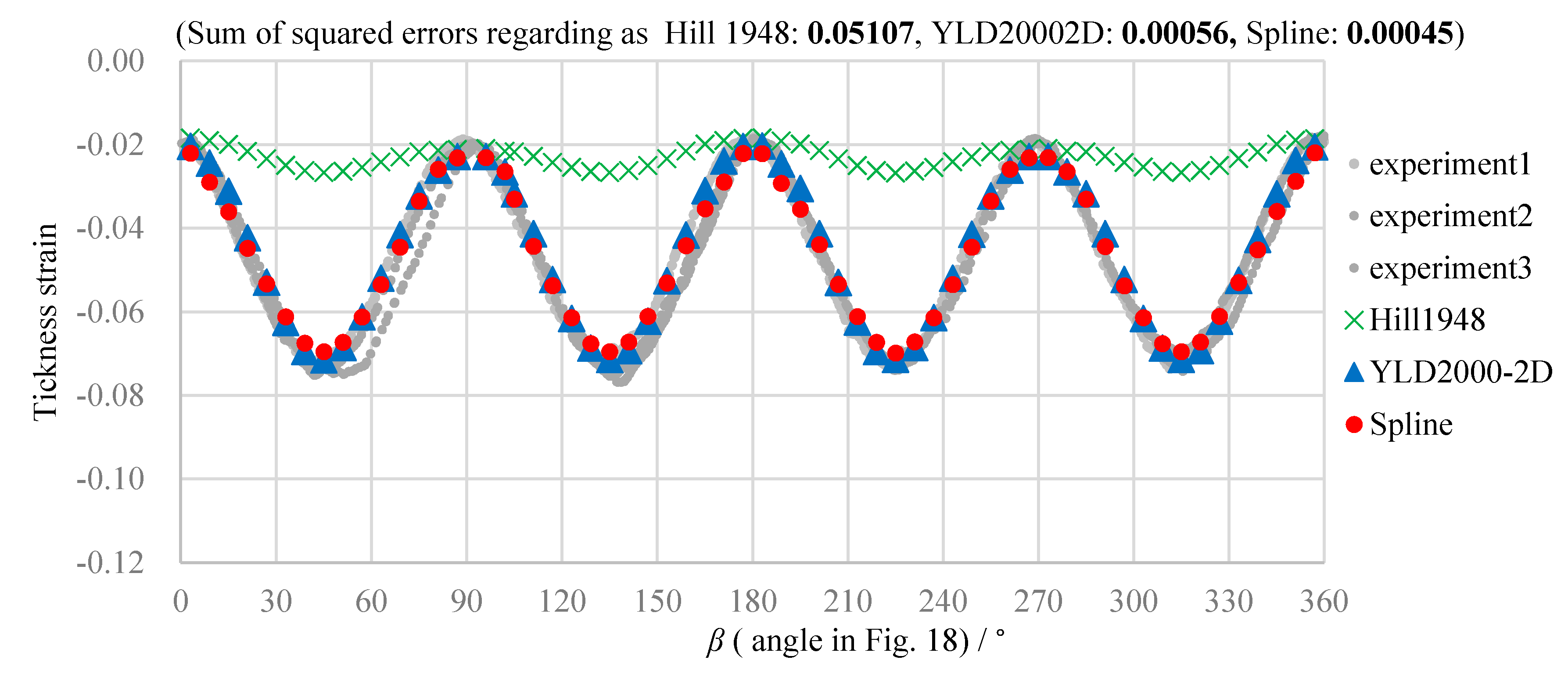
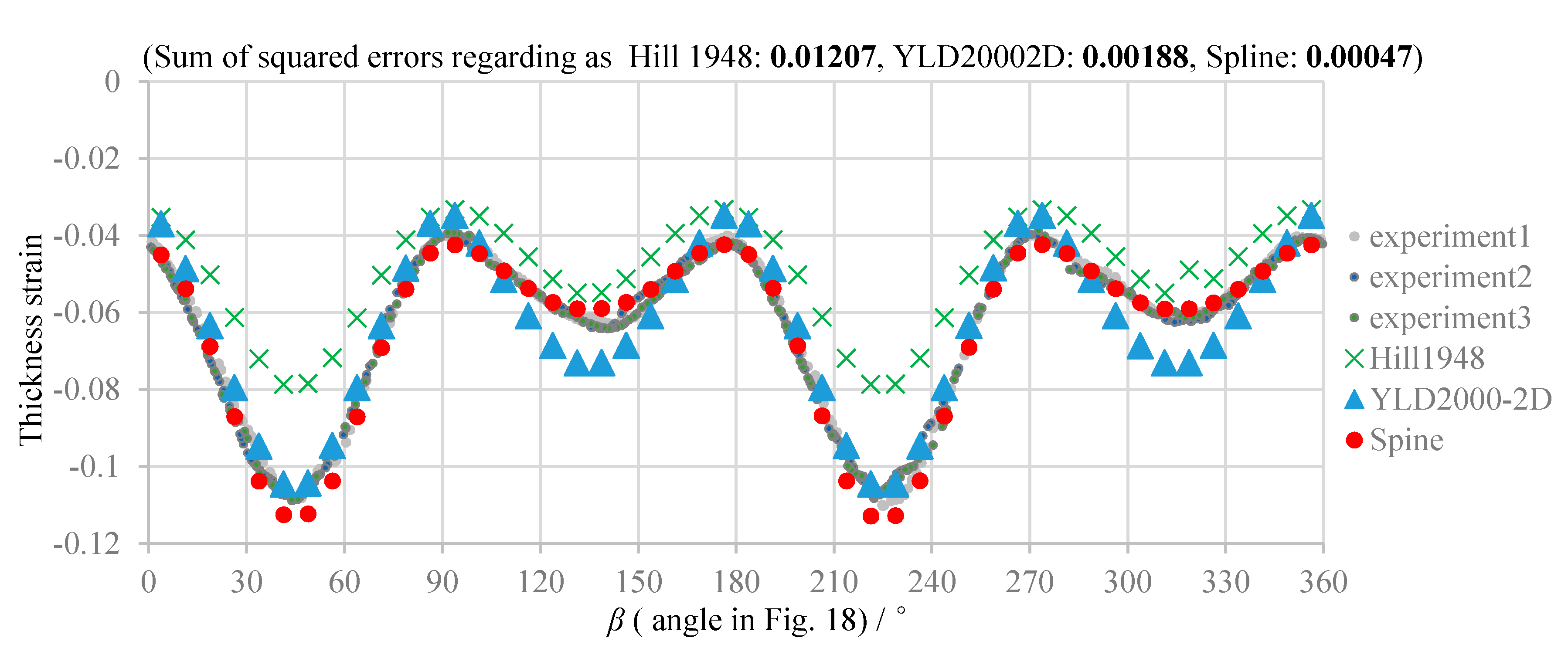
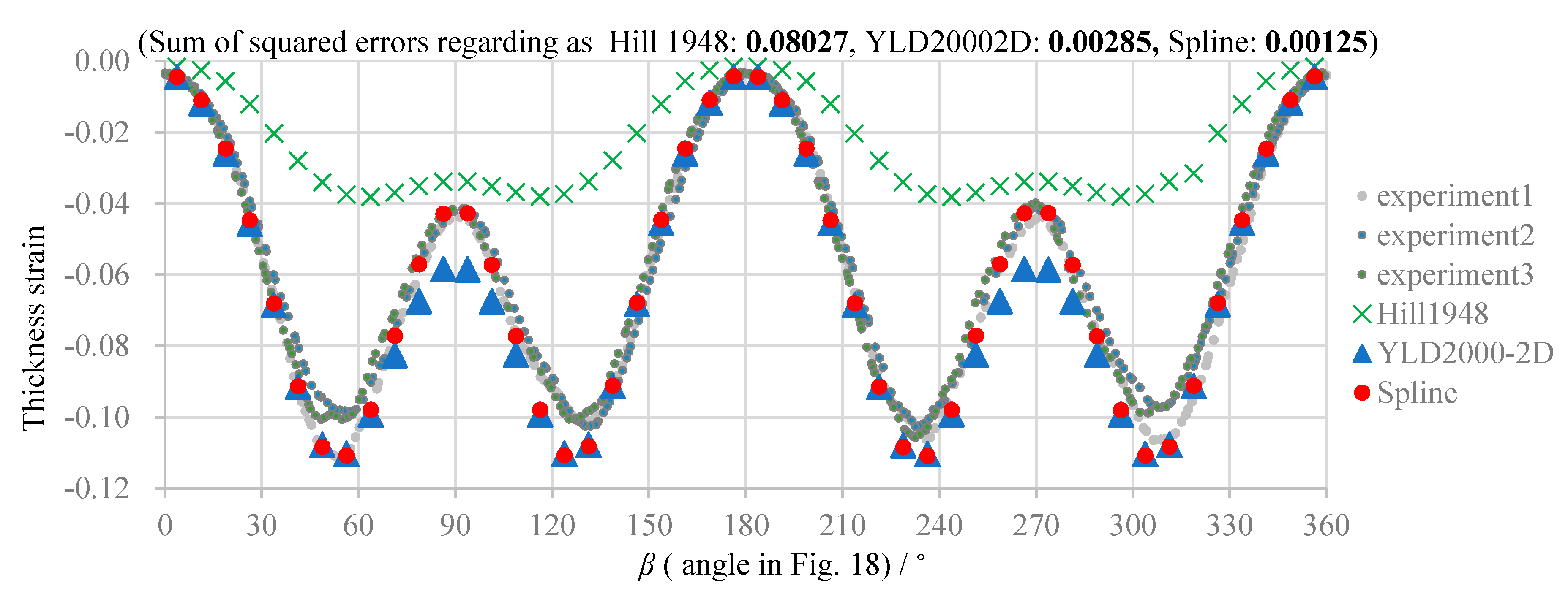
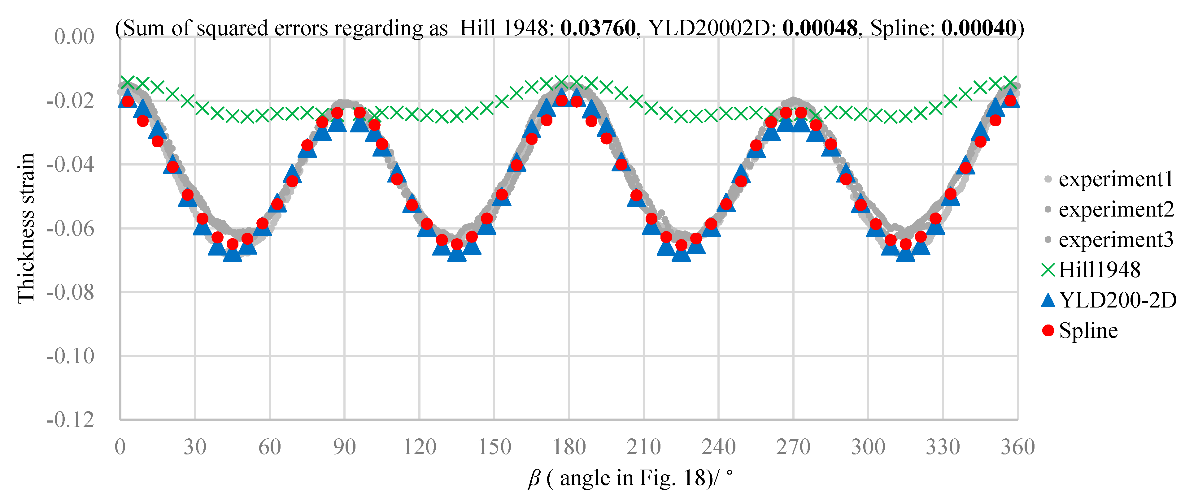
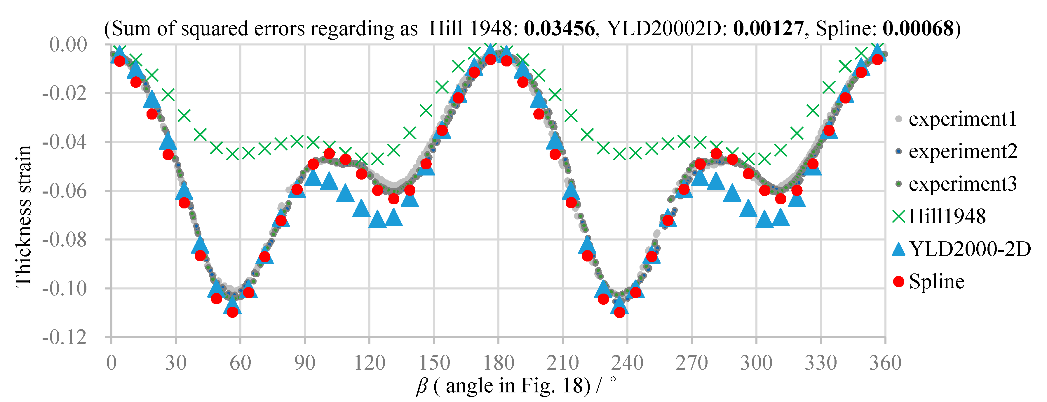
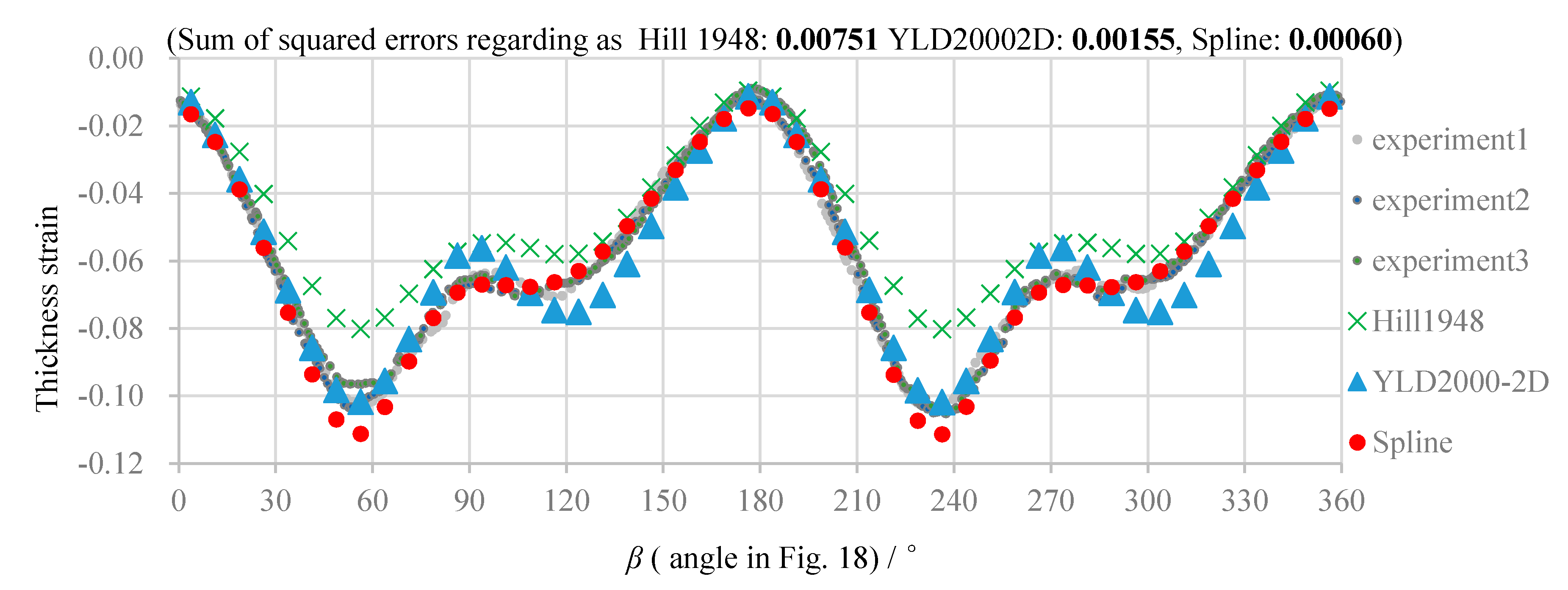
5.3. Comparison of Numerical and Experimental Results

The total force of the step, where the maximum effective plastic strain of the simulation results of the spline yield function was 0.15, was taken as a reference load force to match the conditions of the simulation and experiment. The step corresponding to this load force was selected from the experiment and the simulation results of the other models. The effective plastic strain of 0.15 was taken as the reference effective plastic strain, because the stress-strain curve does not include the Voce approximation. The thickness strain contours of the experiment and the simulation results of the considered yield functions are shown in Figure 17. For numerical comparison, circles are defined for evaluation as shown in Figure 18. These positions were determined in the initial state before applying the displacement. The horizontal axis of the graph for numerical comparison (Figure 18) is β, which is in the range from 0° to 360°. Comparisons of numerical and experimental results of thickness distributions are shown in Figure 19, Figure 20, Figure 21, Figure 22, Figure 23, Figure 24, Figure 25, Figure 26 and Figure 27. The sum of the squared errors between experimental averages and simulation results for each case are also shown to quantify the predictive accuracy; The smaller sum of squared errors means better prediction.
Comparisons of the thickness strain distributions in Figure 19, Figure 20, Figure 21, Figure 22, Figure 23, Figure 24, Figure 25, Figure 26 and Figure 27 reveal that the spline yield function are the most accurate yield function among the three. Moreover, not only qualitative trends but also quantitative values of the simulation results are approximately equal to the experimental results in all conditions. The average of the sum of squared errors between the experimental averages and simulation results for three circles under six different conditions are shown in Table 6, which support the above conclusion. The YLD2000-2D function generally has high accuracy, but this is reduced in circles 1 and 2, close to the hole edge, in experiments A and B. The maximum predicted values of the thickness strain at approximately 90° or 270° deviate from the experimental values. Furthermore, the positions of the predicted maximum strain at approximately 90° and 270° in experiment D deviate from those in the experiment. There were no peaks at 90° and 270° of circle 1 in experiment F; however, the calculation result of YLD2000-2D had different upper and lower peaks from the experiments. The prediction accuracy of the Hill 1948 yield function is poor in the experiment A, B, and D. However, the results at 45° are in good agreement, which we attribute to the equal load on both axes, which is caused by symmetry of orthotropic anisotropy for the rolled material.

6. Concluding Remarks

The prediction accuracy of anisotropic yield functions was evaluated using an in plane biaxial forming tensile test. For the investigation of our proposed yield function proposed and conventional models, we used the aluminum alloy sheets of A6116-T4. The key messages of this work are summarized as follows:
  • A method for determining the parameters of the spline yield function has been developed, which includes a pseudo plane strain stress test by using inverse analysis.
  • For the evaluation of the prediction accuracy of the yield function, an in-plane cruciform tensile test was conducted. This kind of test is appropriate, because it is frictionless and free of bending.
  • The experimental and simulation results reveal high prediction accuracy of the spline yield function. Hence, the validity of the method for parameter determination is verified.
  • The spline yield function is the most accurate model for all considered conditions of the evaluation.
The good agreement of the spline yield function can be ascribed to the high number of input variables (i.e., the uniaxial stresses in five directions, the equi-biaxial stress, the stresses near the plane-strain stress state in five directions, and strain increment directions at all described stress points). There are some differences in the pseudo plane-strain tensile strength depending on the tensile directions. Only the spline yield function can consider these differences, which leads to the best accurate yield function for this material. The comparison of prediction accuracy does not simply determine the superiority or inferiority of the yield function. It should be recognized that each has different numbers of anisotropic parameters. The YLD2000-2D also shows high accuracy considering that the plane-strain tensile test is not needed. Thus, one fewer test yet high accuracy is a benefit of the YLD2000-2D. In further study, other anisotropic yield functions will be evaluated in this cruciform tensile test.

Author Contributions

Conceptualization, H.T.; Data curation, R.R.C.; Investigation, R.R.C., M.E. and S.V.; Software, T.A.; Supervision, W.V.; Writing—original draft, H.T.; Writing—review and editing, M.E. and S.V. All authors have read and agreed to the published version of the manuscript.

Funding

This research received no external funding.

Acknowledgments

This study became possible using the biaxial tensile test machine, which belongs to the institute of Brünig (Universität der Bundeswehr München). For the permission to use the machine, the authors would like to express their great thanks to Brünig, as well as Gerke and the PhD students who supported the realization of the experiments. Furthermore, the authors would like to express their sincere thanks to the PhD students and staff of the Chair of Metal Forming and Casting of the Technical University of Munich for their support and the manufacturing of the specimens, and to the UACJ corporation for supplying the materials. We thank Adam Brotchie, PhD, from Edanz Group (www.edanzediting.com/ac) for editing a draft of this manuscript.

Conflicts of Interest

The authors declare no conflict of interest.

Appendix A

The convexity of yield locus can be used to check following relationships using the control point B i 0 and the normal vector n i 0 . Both relationships must be satisfied in the same time.
( B ( i + 1 ) 0 B i 0 ) n i 0 < 0
( B i 0 B ( i + 1 ) 0 ) n ( i + 1 ) 0 < 0
The relationship between the principal stresses ( σ 1 , σ 2 ) and the stress components ( σ x x , σ y y , σ x y ) in the global coordinate system are as follows, where θ is the angle between direction of the principal stress σ 1 and the x-axis, which is set to RD.
σ 1 = 1 2 ( σ x x + σ y y + ( σ x x σ y y ) 2 + 4 σ x y 2 )
σ 2 = 1 2 ( σ x x + σ y y ( σ x x σ y y ) 2 + 4 σ x y 2 )
cos 2 θ = σ x x σ y y ( σ x x σ y y ) 2 + 4 σ x y 2
The effective stress σ e q , of the yield function is defined by Equation (A6) using the normalized yield function of Equation (2).
( σ 1 σ 2 ) = σ e q R ( θ , u ) = σ e q ( R 1 ( θ , u ) R 2 ( θ , u ) )
The plastic potential, ϕ , is defined by the following:
ϕ ( σ ) = σ e q ( σ )
When σ 1 and σ 2 are partially differentiated with σ 1 , the following the equations are obtained from Equations (A6) and (A7) because each component is independent.
σ 1 σ 1 = 1 = σ e q R 1 ( θ , u ) σ 1 + ϕ σ 1 R 1 ( θ , u )
σ 2 σ 1 = 0 = σ e q R 2 ( θ , u ) σ 1 + ϕ σ 1 R 2 ( θ , u )
Using partial derivatives of the curve parameter u:
σ e q R 1 ( θ , u ) u u σ 1 + ϕ σ 1 R 1 ( θ , u ) = 1
σ e q R 2 ( θ , u ) u u σ 1 + ϕ σ 1 R 2 ( θ , u ) = 0
When Equations (A10) and (A11) are solved for ϕ / σ 1 and ϕ / σ 2 , following equations are obtained:
ϕ σ 1 = R 2 ( θ , u ) u R 1 ( θ , u ) R 2 ( θ , u ) u R 2 ( θ , u ) R 1 ( θ , u ) u
ϕ σ 2 = R 1 ( θ , u ) u R 1 ( θ , u ) R 2 ( θ , u ) u R 2 ( θ , u ) R 1 ( θ , u ) u
Subsequently, when σ 1 and σ 2 are differentiated with θ:
d σ 1 d θ = 0 = σ e q d R 1 ( θ , u ) d θ + d ϕ d θ R 1 ( θ , u )
d σ 2 d θ = 0 = σ e q d R 2 ( θ , u ) d θ + d ϕ d θ R 2 ( θ , u )
where
d R i ( θ , u ) = R i ( θ , u ) θ d θ + R i ( θ , u ) u d u
Because ϕ / θ and d ϕ / d θ are the same, ϕ / θ are represented from Equations (A14) and (A15):
ϕ θ = σ e q R 1 ( θ , u ) u R 2 ( θ , u ) θ R 1 ( θ , u ) θ R 2 ( θ , u ) u R 1 ( θ , u ) R 2 ( θ , u ) u R 2 ( θ , u ) R 1 ( θ , u ) u
If we set X = ( σ 1 , σ 2 , θ ) , σ = { σ x x ,   σ y y , σ x y } T , the direction of the plastic-strain increment, ϕ / σ is given by:
ϕ σ = ( X σ ) T ϕ X
where ϕ / X is
ϕ X = [ σ 1 σ x x σ 1 σ y y σ 1 σ x y σ 2 σ x x σ 2 σ y y σ 2 σ x y θ σ x x θ σ y y θ σ x y ]
For each component of the Equation (A19), each value is determined from Equations (A3)–(A5).
Finally, the plastic multiplier d λ is determined. The consistency condition during plastic deformation is written as follows, where ε ¯ is the effective plastic strain:
ϕ σ · d σ + ϕ ε ¯ · d ε ¯ = 0
ϕ / ε ¯ is equivalent to σ e q / ε ¯ which corresponds to the slope of a hardening rule. The stress increment is given by:
d σ = C ( d ε d λ ϕ σ )
where C be the elastic tensor, d ε = { d ε x x ,   d ε y y , d ε x y } T is the total strain increment.
The effective plastic-strain increment is given by:
d ε ¯ = ( 2 3 d λ ϕ σ · d λ ϕ σ ) 1 2
d λ is obtained as follows:
d λ = ϕ σ C d ε ϕ σ C ϕ σ ϕ ε ¯ ( 2 3 ϕ σ ϕ σ ) 1 2
Thus, the plastic-strain increment, d ε = d λ ( ϕ / σ ) , is explicitly obtained.

References

  1. Hill, R. A theory of the yielding and plastic flow of anisotropic metals. Proc. R. Soc. Lond. 1948, 193, 281–297. [Google Scholar]
  2. Barlat, F.; Brem, J.C.; Yoon, J.W.; Chung, K.; Dick, R.E.; Lege, D.J.; Pourboghrat, F.; Choi, S.H.; Chu, E. Plane stress yield function for aluminum alloy sheets—Part 1: Theory. Int. J. Plast. 2003, 19, 1297–1319. [Google Scholar] [CrossRef]
  3. Tsutamori, H.; Iizuka, E.; Amaishi, T.; Sato, K.; Ogihara, Y.; Miyamoto, J. Plane Stress Yield Function Described by 3rd-degree Spline Curves Considering Differential Work Hardening. J. Jpn. Soc. Technol. Plast. 2016, 657–662, 245–251. (In Japanese) [Google Scholar] [CrossRef] [Green Version]
  4. Iizuka, E.; Hashimoto, K.; Kuwabara, T. Effects of anisotropic yield functions on the accuracy of forming simulations of hole expansion. Procedia Eng. 2014, 81, 2433–2438. [Google Scholar] [CrossRef] [Green Version]
  5. Panich, S.; Uthaisangsuk, V.; Suranuntchai, S.; Jirathearanat, S. Anisotropic Plastic Behavior of TRIP 780 Steel Sheet in Hole Expansion Test. Key Eng. Mater. 2012, 504–506, 89–94. [Google Scholar] [CrossRef]
  6. Kuwabara, T.; Mori, T.; Asano, M.; Hakoyama, T.; Barlat, F. Material modeling of 6016-O and 6016-T4 aluminum alloy sheets and application to hole expansion forming simulation. Int. J. Plast. 2017, 93, 164–186. [Google Scholar] [CrossRef]
  7. Kuwabara, T.; Hashimoto, K.; Iizuka, E.; Yoon, J.W. Effect of anisotropic yield functions on the accuracy of hole expansion simulations. J. Mater. Process. Technol. 2011, 211, 475–481. [Google Scholar] [CrossRef]
  8. Hol, J.; Alfaro MV, C.; Rooij, M.B.; Meinders, T. Advanced friction modeling for sheet metal forming. Wear 2012, 286–287, 66–78. [Google Scholar] [CrossRef] [Green Version]
  9. Wang, W.; Zhao, Y.; Wang, Z.; Hua, M.; Wei, X. A study on variable friction model in sheet metal forming with advanced high strength steels. Tribol. Int. 2016, 93, 17–28. [Google Scholar] [CrossRef]
  10. Hashimoto, K.; Isogai, E.; Yoshida, T.; Kuriyama, Y.; Ito, K. Finite Element Analysis of Sheet Metal Forming Taking Account of Nonlinear Friction Model—Assessment of Sheet Formability by Nonlinear Friction Model III. J. Jpn. Soc. Technol. Plast. 2007, 549–573, 995–999. (In Japanese) [Google Scholar]
  11. Kuwabara, T.; Ichikawa, K. Hale Expansion Simulation Considering the Differential Hardening of a Sheet Metal. Rom. J. Technol. Sci. 2015, 60, 63–81. [Google Scholar]
  12. Suzuki, T.; Okamura, K.; Capilla, G.; Hamasaki, H.; Yoshida, F. Effect of anisotropy evolution on circular and oval hole expansion behavior of high-strength steel sheets. Int. J. Mech. Sci. 2018, 146–147, 556–570. [Google Scholar] [CrossRef]
  13. Yoshida, F.; Uemori, K.; Fujiwara, K. Elastic-plastic behavior of steel sheets under in-plane cyclic tension-compression at large strain. Int. J. Plast. 2002, 18, 633–659. [Google Scholar] [CrossRef]
  14. Logan, R.W.; Hosford, W.F. Upper-Bound Anisotropic yield Locus Calculations Assuming <1 1 1 >—Pencil Glide. Int. J. Mech. Sci. 1980, 22, 419–430. [Google Scholar] [CrossRef] [Green Version]
  15. Vegter, H.; Boogaard, A.H. A plane stress yield function for anisotropic sheet material by interpolation of biaxial stress states. Int. J. Plast. 2006, 22, 557–580. [Google Scholar] [CrossRef]
  16. Amaishi, T.; Tsutamori, H.; Iizuka, I.; Sato, K.; Ogihara, Y.; Matsui, Y. A Yield Function for Anisotropic Sheet Material Described by 3rd-Degree Spline Curve and its Applications. Key Eng. Mater. 2017, 725, 653–658. [Google Scholar] [CrossRef]
  17. Amaishi, T.; Tsutamori, H.; Nishiwaki, T.; Kimoto, T. A Plane Stress Yield Function by Multi-Segment Third Order Beézier curves. Key Eng. Mater. 2018, 794, 163–168. [Google Scholar] [CrossRef]
  18. Brünig, M.; Brenner, D.; Gerke, S. Stress state dependence of ductile damage and fracture behavior: Experiments and numerical simulations. Eng. Fract. Mech. 2015, 141, 152–169. [Google Scholar] [CrossRef]
  19. Bathe, K.J.; Dvorkin, E.N. A four-node plate bending element based on Mindlin/Reissner plate theory and a mixed interpolation. Int. J. Numer. Method Eng. 1985, 21, 367–383. [Google Scholar] [CrossRef]
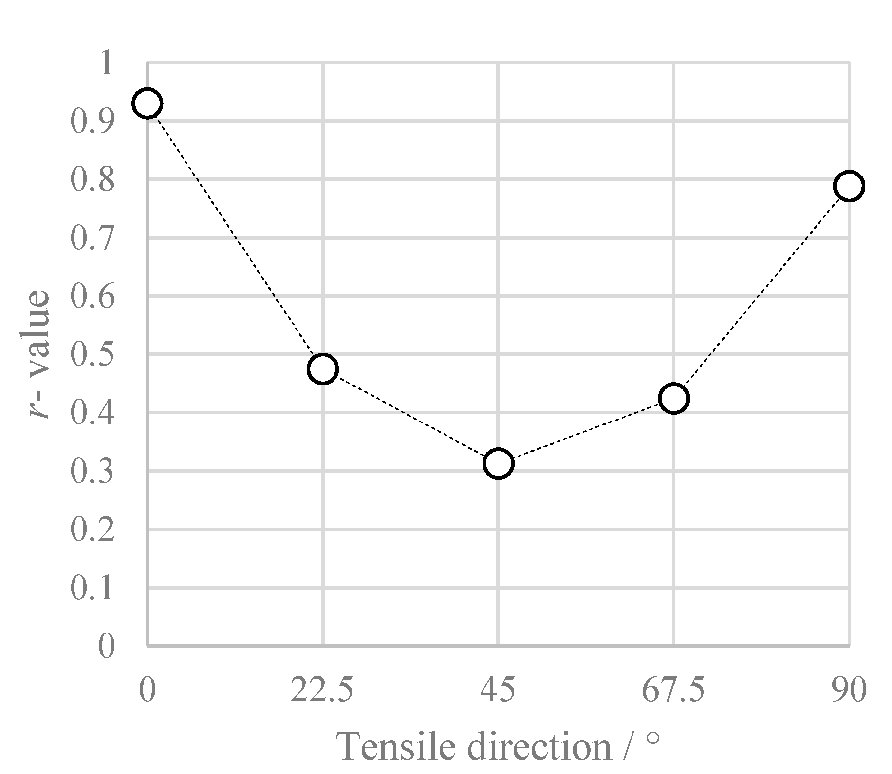
Figure 1. Spline yield function composed of Bézier curves.
Jmmp 04 00043 g001
Figure 2. Spline basis function for interpolation.
Jmmp 04 00043 g002
Figure 3. Locations of A 1 A 3 and B i 0 which are used as parameters pk and qk.
Jmmp 04 00043 g003
Figure 4. Stress-strain curve under uniaxial stress in the 0° direction (a), Zoomed S-S curve (b).
Jmmp 04 00043 g004
Figure 5. Distribution of r-value.
Jmmp 04 00043 g005
Figure 6. Geometry of specimen.
Jmmp 04 00043 g006
Figure 7. Maximum principal strain distribution.
Jmmp 04 00043 g007
Figure 8. Nominal stress corresponding to the average strain.
Jmmp 04 00043 g008
Figure 9. Width strain at P2 respect to the average strain.
Jmmp 04 00043 g009
Figure 10. A finite element (FE) model used for inverse analysis.
Jmmp 04 00043 g010
Figure 11. Comparisons between experiments and simulation result after optimization for the 0° direction. (a) Tensile force respect to average strain. (b) Strain of width at P2 respect to average strain.
Jmmp 04 00043 g011
Figure 12. Comparison of the shape of normalized equi-plastic work surface for each yield function.
Jmmp 04 00043 g012
Figure 13. Shape of normalized equi-plastic work surface in principal stress space when the horizontal axis was 22.5° from the RD.
Jmmp 04 00043 g013
Figure 14. Shape of normalized equi-plastic work surface in principal stress space when the horizontal axis was 45° from the RD.
Jmmp 04 00043 g014
Figure 15. Biaxial tensile testing machine.
Jmmp 04 00043 g015
Figure 16. Geometry of cruciform specimen.
Jmmp 04 00043 g016
Figure 17. Comparison of thickness strain distribution contours of experimental condition F.
Jmmp 04 00043 g017
Figure 18. Location of circles the analyzed in the measurements.
Jmmp 04 00043 g018
Figure 19. Comparison of thickness strain distributions on circle 1 in experimental condition A.
Jmmp 04 00043 g019
Figure 20. Comparison of thickness strain distributions on circle 2 in experimental condition A.
Jmmp 04 00043 g020
Figure 21. Comparison of thickness strain distributions on circle 3 in experimental condition A.
Jmmp 04 00043 g021
Figure 22. Comparison of thickness strain distributions on circle 1 in experimental condition B.
Jmmp 04 00043 g022
Figure 23. Comparison of thickness strain distributions on circle 2 in experimental condition B.
Jmmp 04 00043 g023
Figure 24. Comparison of thickness strain distributions on circle 3 in experimental condition B.
Jmmp 04 00043 g024
Figure 25. Comparison of thickness strain distributions on circle 1 in experiment condition D.
Jmmp 04 00043 g025
Figure 26. Comparison of thickness strain distributions on circle 1 in experimental condition E.
Jmmp 04 00043 g026
Figure 27. Thickness strain distributions on circle 1 in experimental condition F.
Jmmp 04 00043 g027
Table 1. Properties of the A6116 specimen.
Tensile Direction/°Yield Strength (0.2%)/MPaTensile Strength/MPar (εp = 0.05) r ˜ Normalized Stress (εp = 0.05)
0144.15262.660.9300.9091.000
22.5140.82256.550.4750.4870.972
45140.37254.880.3130.3100.962
67.5137.42250.070.4240.4180.956
90137.30251.320.7880.7360.980
Table 2. Equi-biaxial stress and strain increment.
Normalized Stress (εp = 0.05) Strain   Increment   Ratio   ( r b = d ε y / d ε x )   ( ε p = 0.05 )
0.9811.005
Table 3. Parameters pk and qk for spline yield function.
k01234
Angle from RD/°022.54567.590
pk0.4580.3370.2000.2600.342
qk0.3280.2890.2830.2760.238
Table 4. Experimental conditions.
Type of Experimentα/° (Angle between Horizontal Arm and RD)Displacement RatioNumber of Repetitions
A0.01:13
B0.02:13
C22.51:13
D22.52:13
E45.01:13
F45.02:13
Table 5. Material parameters for YLD 2000-2D.
α 1 α 2 α 3 α 4 α 5 α 6 α 7 α 8 m
0.97601.03670.94591.04001.01661.05530.90831.19488
Table 6. Comparison of sum of squared errors among the yield functions.
Hill 1948YLD2000-2DSpline Yield Function
Average of sum of squared errors between experimental averages and simulation results for 3 circles of 6 conditions in Table 40.030320.001140.00063

