Method for Analytical Calculation of the Formability from Metallic Bipolar Plates

Abstract

The constructive design of a flow field layout and the channel cross section parameters from a metallic half- or bipolar plate can have a significant influence on the performance characteristics of a fuel cell. One important aspect in the dimensioning of the channel geometry of half plates is the technical forming feasibility. In this article, first an equation is presented, which enables an analytical calculation of the channel parameters. Hereby, continuing calculations with parameter variations will be possible. Furthermore, the formability of the channel geometry of metallic half plates is evaluated through numerical and experimental investigations. Based on the results, an analytical model approach will be derived that enables an appraisal of the formability from channel cross section contours in an early development state. As a final step, the results of the numerical investigations and the analytical calculation method are compared and evaluated with the results of experimental investigations and other publications. It will be shown, that the derived analytical model approach has a good approximation compared to the effects and results from the numerical and experimental analysis. In particular, the assessment of whether a channel cross section can be manufactured safely is a result with high probability of the analytical model approach. Imprecisions happen, especially in variants with extreme geometries, for example, with very small radii or a huge channel depth. For this kind of variations, the analytical model behaves too sensitively, which makes it more difficult to estimate the damage effects. However, at an early development state, the analytical model offers a good method to get a pre-evaluation of the formability of channel cross sections with a simultaneous parameter variation possibility.

1. Introduction

The fuel cell technology presents one possibility to achieve a future with less pollutant emission. In particular, the fuel cell type low temperature polymer electrolyte membrane fuel cell (LT-PEM-FC) is nowadays the focus of many developments, as well as in stationary, portable and mobile application fields. The advantage of those fuel cells are, among others, the low operational temperature, good startup performance, high efficiency and high power density [1,2,3]. Due to the mentioned diversity of application fields, a requirement-oriented design is suggested.

Normalized and standardized guidelines are available only rudimentary according to the actual state of science and technology. Main criteria by designing channel plates for fuel cell applications are mostly an effective utilization of a given active area, a low pressure drop over the flow field, as well as a homogeny media distribution. At the same time, especially the water management (defined removal of reaction water from membrane area) in a flow field must be considered. Areas of the flow field with undercut contours or stagnant media flow have to be avoided. The channels must be dimensioned exactly through given load requirements so that a sufficient media supply and media flow can be guaranteed. On the other side, the channels should not be too big to prevent an excessive intrusion of the gas diffusion layer (GDL) in the channel cross section as a result of clamping force. With this kind of effect, the channels are likely to be narrowed and thus, blocked. A uniform pressure distribution over the flow field forms a further requirement, which can be influenced by means of the targeted design of the flow field layout.

1.1. Forming and Formability of Metallic Channel Plates

Taking into account all of the above-mentioned aspects, in the manufacturing point of view, the achievement of a save formability of the channel cross section structure plays an important role for the dimensioning of a large-scale metallic bipolar plate production. In an early development phase, it can be very helpful to get a rough estimation of the forming feasibility of a channel cross-sectional contour. With this kind of information, it is possible to compare alternative geometries, to increase the development potential and to identify critical variants at an early stage. For an efficient implementation, a fast and simple calculation option is necessary and for this reason, should not be based on numerical approaches, but can provide a reliable statement about formability in a time-efficient manner. The aim of this work is the derivation of an analytical equation for the description of the trend behavior of the forming feasibility. Therefore, different channel cross-sectional contours can be taken into account while defined channel parameters can be variated. The equation approach is consciously not based on physical principles, but reflects the trend behavior for the formability of different variants. This quick and easy-to-use method represents an innovation in the current state of science and technology, which has not been presented yet.

Typical manufacturing methods in the current state of the art are mechanical deep drawing [4,5,6,7,8,9,10,11], hydroforming [4,12] or rubber pad forming [4,13,14,15]. The basic objective of all manufacturing processes is a precise and accurate forming result of the desired channel cross section profile. A particular challenge hereby is usually the prevention of excessive local thinning (e.g., in radii areas) to avoid cracks in the formed product. The damage of the plate directly leads to the loss of function.

The formability of these metallic channel half-plates has been studied scientifically. In addition to some literature with experimental focus, technical investigations can be found, especially in the field of numerical simulations like the Finite Element Method (FEM).

Peng et al. [4] give a broad overview of scientific results of numerous publications in recent years on the subject of forming and formability of metallic channel half-plates. Different production and coating methods as well as assembly and scaling properties are listed.

Zhao and Peng [5] conducted forming experiments on nine sample geometries and investigated the influence of different channel parameters on formability. They also developed a calculation model for micro forming process. The forming experiments were carried out by mechanical deep drawing until the first crack of the channel half-plate occurs. As a result, the maximum possible channel depths per channel cross-sectional contour was determined.

Qiu et al. [6] investigated the forming process of 40 samples with different geometries experimentally by mechanical deep drawing. Again, the forming operations in each drawing process were conducted to the maximum possible channel depth. The results were used to assess the sensitivity of individual channel parameters to formability. It turned out that above all the measurements, the dimensions of the radii and the width of the drawing gap between the forming dies have a significant influence on the formability. Continuously, complete channel half-plates were produced and the forming quality of the channel structures as well as of the entire plates was evaluated with reference to assembly aspects.

Hu et al. [7] analyzed the influence of geometrical parameters on the formability of metallic bipolar plates in numerical and experimental investigations. It was established that a maximum channel depth of $0.56 \mathrm{mm}$ by a given layout with a sheet thickness of $0.15 \mathrm{mm}$ can be achieved by stamping forming technology, if the channel parameters channel length and land width are in the range of $0.5 \mathrm{mm}$ to $1.5 \mathrm{mm}$. In general, a larger channel length, land width and a smaller channel depth as well as larger channel radii shows a positive effect on the formability. The initial blank and the forming parameters themselves (e.g., forming speed) have a significant influence too.

Xu et al. [8] investigated the formability of channel structures of different geometries by means of a 2D FE model approach. Here, three series of experiments were carried out with different parameters. In each testing cycle, the width of the mold on the upper die was varied from $0.6 \mathrm{mm}$ to $1.0 \mathrm{mm}$, the channel height from $0.4 \mathrm{mm}$ to $0.7 \mathrm{mm}$ and the radii in the range of $0.15 \mathrm{mm}$ to $0.30 \mathrm{mm}$. Subsequently, the minimum sheet thicknesses was evaluated. In all forming simulations, the largest loads occurred in the radii areas during the forming process.

Khatir et al. [9] realized experimental forming tests by means of mechanical deep drawing. The main object of the study was the comparison of the forming capacity with and without additional lubricant. It could be observed that the formability with the use of a lubricant leads to significantly greater forming depths.

Zhou and Chen [10] used FE simulations and experimental tests to investigate the forming behavior of single- and three-channel samples. It could be identified that larger radii and a larger channel flank angle generally have a favorable effect on the formability. On the other hand, the channel length has a rather small influence on the stress distribution and thus, the formability.

Peng et al. [13] analyzed the forming behavior of metallic half-plates by means of rubber pad forming technology in numerical FE simulations and subsequent experimental implementations. Within the framework of the FE investigations, five channel geometries were evaluated. The subsequent experimental implementation of a metallic channel half-plate validates the simulations. In principle, the feasibility of manufacturing metallic bipolar plates by means of rubber pad forming was demonstrated.

1.2. Investigations of Channel cross Sections

In addition to the listed research on the formability of metallic channel half-plates, other articles also show assumptions and models for the description of the channel geometry. Those differ mainly for the basic channel cross section structure considered. In most cases, idealized square channel structures are assumed. These kind of channels can be found in various publications [16,17,18,19,20,21,22]. Different variation parameters were assumed, for example the channel width, the channel depth and the width of land or rib. Through this, the channel-to-rib-ratio varies. In the publication by Zeng et al. [23], a channel ground deviating from the channel width was also defined. This resulted in a channel flank angle, so channel cross section can be trapezoidal.

Channel cross section descriptions based on manufacturing and thus tool parameters can be found in the publications [6,7,9]. For example, Khatir et al. [9] defined Parameters on the upper and lower dies or the forming punch of the forming tool, resulting in a reshaped channel cross section. Among others, a punch height, a punch flank angle, a punch land width, a punch ground width and an inner and outer radius are set. In addition, a parameter for the sheet thickness was defined.

More detailed model descriptions based on the channel cross section using channel parameters can be found in the following works [24,25,26]. For example, in [25], Breuer defines the channel parameters: channel height, land width, channel flank angle, inner and outer radius and sheet thickness. The channel width and the channel ground are not explicitly defined, but given implicitly due to the geometrically determined shape of the channel cross section through the correlation between all of the channel parameters.

2. Materials and Methods

On the basis of the different approaches to the channel parameter description listed in the previous section, a first aim of this work was the achievement of a general description on the usual channel parameters. For this purpose, a standardized equation approach is derived below and will be used later in other cases.

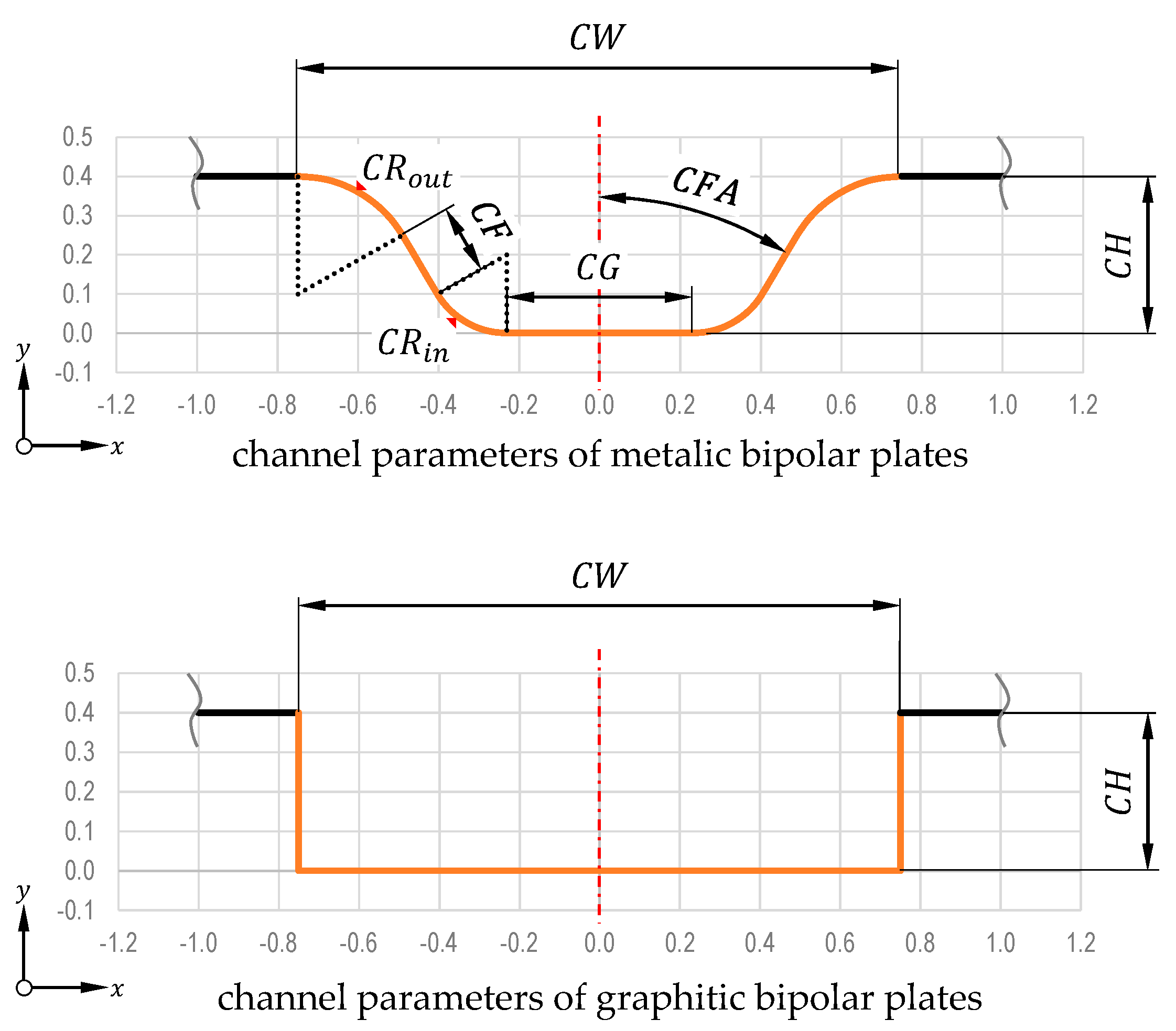
2.1. Definition of the Channel Parameters

2.1.1. Equation of Channel Parameters

In this work, primarily channel geometries of metallic bipolar plates are examined, which are manufactured by mechanical deep drawing. However, the listed equations also apply to the calculation of graphitic channel structures (e.g., milled channels).

The channel parameters result from the shape of the forming tools, see following Figure 1. The forming tools usually contain a punch ① and a die ②. These define the channel ground width, the land or rib width ③ as well as the outer and inner radii. The orientation of the channel flank angle can be influenced by the height ④ and the distance between punch and die. In this context, the required drawing gap ⑤ is set, which defines the distance between punch and die and should be at least as wide as the initial sheet thickness. In addition to the stamp geometries, the sheet thickness of the blank is also decisive for the shape of the channel cross section contour, especially in relation to the shape of the outer radius and the orientation of the channel flank.

The channel cross section parameters which were obtained from this are defined as shown in Figure 2.

The channel width $CW$ hereby illustrates the distance between the outer points of the outer radii. The channel ground $CG$ shows the distance between the inner points of the inner radii. The channel height $CH$ defines the distance from the channel ground to the top. $C{R}_{out}$ describes the outer radius and $C{R}_{in}$ the inner radius. The angle between a channel flank and the virtual vertical centerline of a channel is defined as the channel flank angle $CFA$. These channel parameters stand in direct relation to each other and therefore, cannot be varied arbitrarily.

2.1.2. Approach and Derivation

To develop a general calculation equation, all previously defined channel parameters must be combined in a relation to each other. For this purpose, the angle-relations and the composition of the channel flank are additionally clarified in Figure 3.

It can be seen that the channel flank angle $CFA$ is presented in angular relations in several areas. In addition, a horizontal component $C{F}_x$ and a vertical component $C{F}_y$ are defined for the channel flank $CF$.

The equation is derived from the width balance of the channel. It follows:

$$CW=CG+2 \cdot \left[C{R}_{out}\cos \left(CFA\right)+C{R}_{in}\cos \left(CFA\right)+C{F}_x\right]$$

(1)

Due to the symmetrical structure of the channel cross section, the width segments of the outer and inner radii as well as the channel flank are included twice in the calculation. The horizontal component $C{F}_x$ of the channel flank can be described in more detail by means of a trigonometric relation via the vertical component $C{F}_y$:

$$C{F}_x=C{F}_y\cdot \tan \left(CFA\right)$$

(2)

The vertical component of the channel flank $C{F}_y$ is further calculated from a height balance of the channel cross section. Here, the relation between the channel height $CH$ and the proportional vertical components of the outer and inner radii results in

$$C{F}_y=CH-\left(C{R}_{out}-C{R}_{out}\sin \left(CFA\right)\right)-\left(C{R}_{in}-C{R}_{in}\sin \left(CFA\right)\right)$$

(3)

Taking into account the formulated Equations (1), (2) and (3), the general channel parameter equation results as follows [27]:

$$0=CW-CG-CH\cdot 2\tan \left(CFA\right)+\left(C{R}_{out}+C{R}_{in}\right)\cdot \left(2\frac{\sin \left(CFA\right)-1}{\cos \left(CFA\right)}\right)$$

(4)

This always relies on ideally shaped channels according to the description above in Figure 2. From the Equation (4), it is possible to see that five of the six parameters can be varied—the remaining unknown parameter was gained from the calculation of the given equation conclusively.

2.1.3. Validity and Restrictions

The previously mentioned channel parameter equation is generally valid and can also be used to calculate milled channel structures. In order to ensure the validity of the described equation, the respective parameters have to be in defined and technically meaningful ranges. The following conditions must be valid:

• $C\mathrm{W}>0\mathrm{mm}$
• $CH>0\mathrm{mm}$
• $CG\ge 0\mathrm{mm}$
• $C{R}_{out}\ge 0\mathrm{mm}$
• $C{R}_{in}\ge 0\mathrm{mm}$
• $0°\le CFA<90°$
• $CW\ge CG$

In addition, the restriction $CF\ge 0\mathrm{mm}$ must be fulfilled. The channel flank is calculated as follows:

$$CF=\frac{CH-\left(C{R}_{out}+C{R}_{in}\right)\cdot \left(1-\sin \left(CFA\right)\right)}{\cos \left(CFA\right)}$$

(5)

The presented equation for the channel flank can be used analogously for the calculation of the channel structure of milled bipolar plates. Here, $C{R}_{out}$ and $C{R}_{in} = 0 \mathrm{mm}$ as well as $CFA = 0°$. The Equation (5) is simplified by this and results in $CF =CH$.

2.2. Numerical Simulation Model and Forming Experiments

2.2.1. Numerical Approach and Setup

The numerical simulation was conducted with the FEM forming tool simufact.forming GP 14.0. All tool geometries (punch and die) were imported as 2D IGES-files (Figure 4). For both the simulation model and the experimental setup, the channel parameters were defined as follows:

• $C\mathrm{W}=1.655\mathrm{mm}$
• $CH=0.500\mathrm{mm}$
• $CG=0.500\mathrm{mm}$
• $C{R}_{out}=0.300\mathrm{mm}$
• $C{R}_{in}=0.200\mathrm{mm}$
• $CFA=30°$

The lateral material flow in X-direction on the edges of the specimen was blocked by boundary conditions and the drawing gap was closed completely to the height of the initial metal foil to achieve a critical forming behavior. For the friction, a coulomb model was used with the factor of $0.1$, which is usual for forming contacts between tools and stainless steels. A discretization with an edge length of $0.1\mathrm{mm}$ and quad-elements was applied to the workpiece. The contact bodies were defined as rigid and the punch was velocity controlled ($0.5 \mathrm{mm}/\mathrm{s}$). To provide a realistic flow curve, the 316 L (1.4404) stainless steel was analyzed in experimental bulge tests directly with the same batch which was used for the real forming experiments (Figure 5).

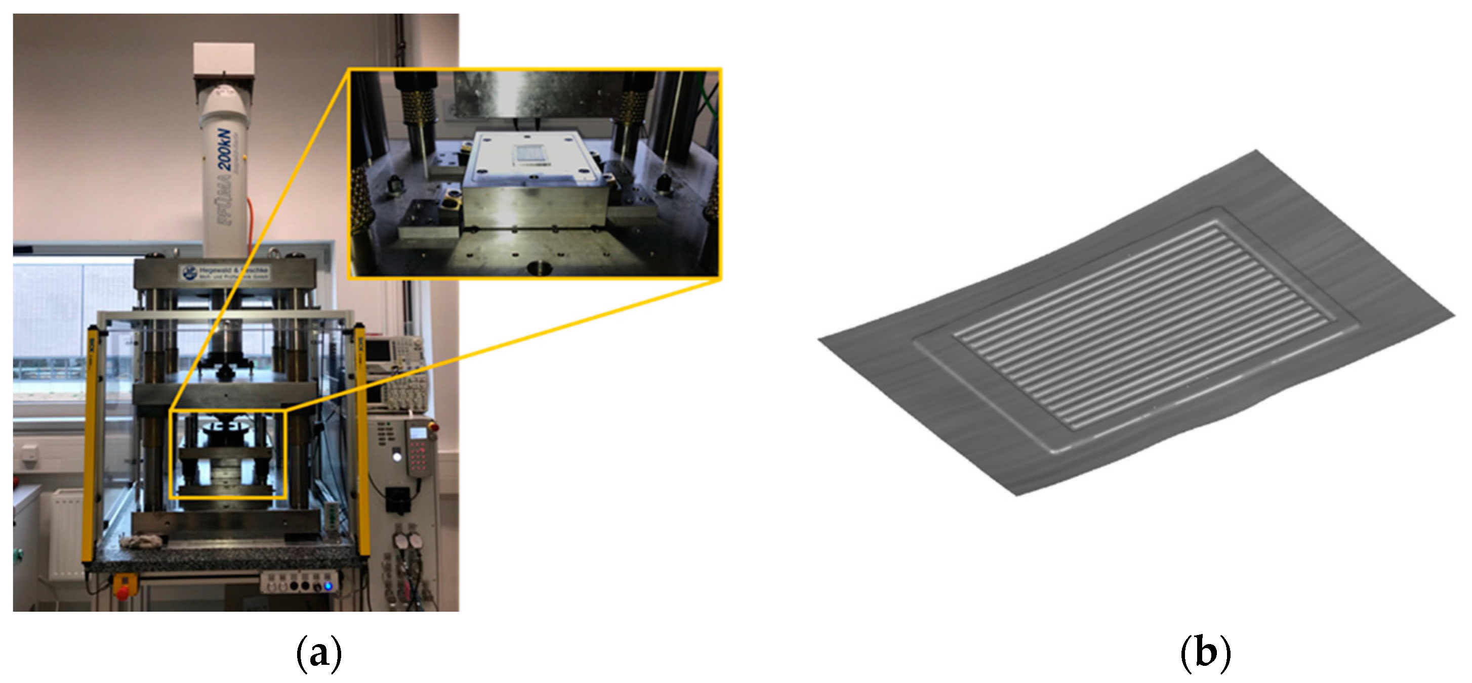
2.2.2. Experimental Setup

The forming experiments were performed on a precision forming machine (P.FÜ.MA; Hegewald & Peschke Meß- und Prüftechnik GmbH), which was provided by the Professorship for Micromanu-facturing Technologies of the Technical University Chemnitz. This machine is a four-column servo press which is specialized on precision forming processes because of its high accuracy (Figure 6a). Prior to the forming experiments the alignment of punch and die was guaranteed by the use of pressure indicating films which were formed between the dies without a workpiece. Thus, these foils were able to indicate an eccentrically positioning of the tools with a colored marking in areas with higher contact pressure. For the conduction of the experiments, the forming speed was defined with $0.5 \mathrm{mm}/\mathrm{s}$ and a reproducible starting point was defined by a $150\mathrm{N}$ pre-load of the punch on the plane metal foil. The formed sample was a bipolar plate dummy in the dimensions of $80\mathrm{mm}$ × $50\mathrm{mm}$, which implements the channel geometries as used for real bipolar plates and as described in Section 2.1.1 (Figure 6b).

The initial material was a 316 L stainless steel with a thickness of $0.1 \mathrm{mm}$, which was the same as used for the material characterization in Section 2.2.1. Subsequently to the forming experiments, the specimen were cut at different spots in the flow field with a Discotom machine to achieve good surface qualities with low thermal influences for the microscopic analyses. The microscopic analyses were performed on an Axiovert 200 MAT microscope with the corresponding software AxioVision of the Carl Zeiss AG. From different positions, five thickness values were measured for three areas in the formed channels and summed up to an average value.

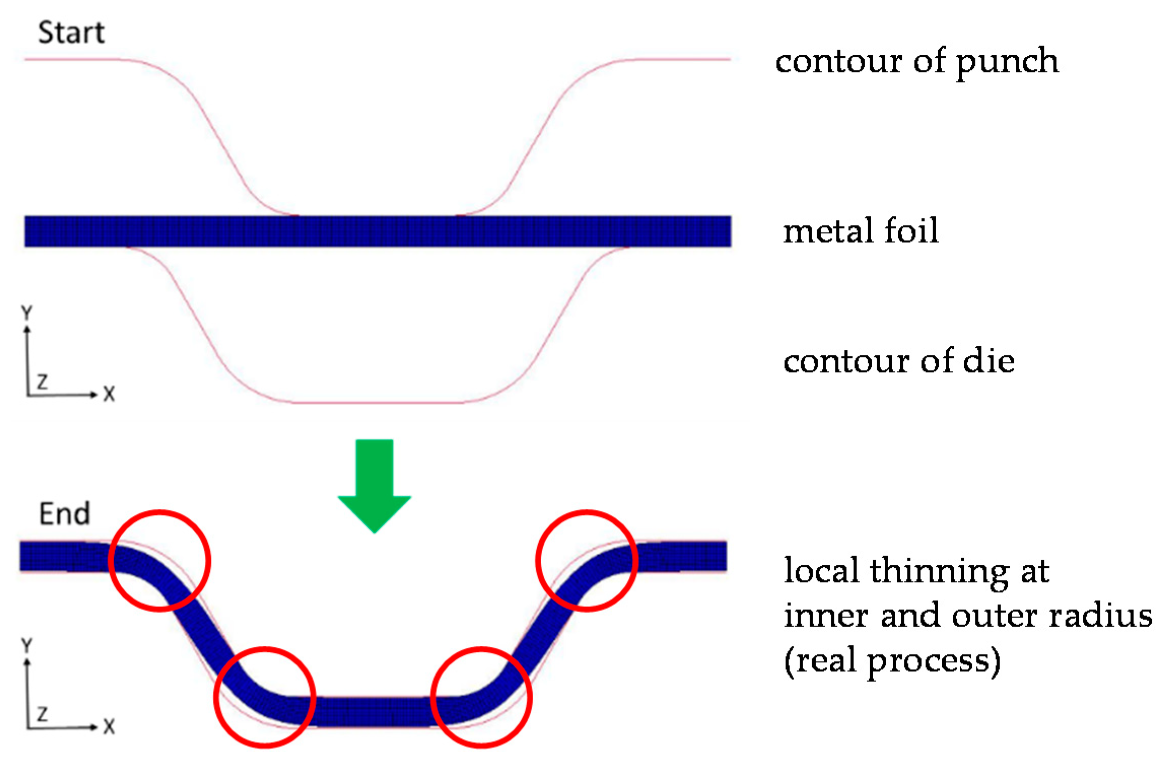
2.2.3. Simulation Results and Validation with Real Process

To implement the numerical model for further process and parameter variations, it has to be calibrated first. The calibration was realized with a direct comparison between the microsection from the forming experiments as described in Section 2.2.2. and the corresponding FEM forming simulation as mentioned in Section 2.2.1 (Figure 7).

The maximum equivalent plastic strain of the simulation lies in the amount of $\phi = 0.49$. All distances for the remaining channel thickness after forming are given as an average of five measured channels and can be seen in

Table 1. Comparison of the remaining channel thickness after forming between experiment and FEM.

Position	Experiment in µm	FEM in µm	Deviation in %
1	74.0	74	0.0
2	83.2	83	0.5
3	77.8	76	2.0

.

Within Table 1, it can be see that there is a very good coincidence between the numerical simulation and the experiments with a maximum deviation of $2\%$. Therefore, the developed simulation setup can be used as a reliable predictive model for the variation of channel geometries.

2.3. Analytical Model

After a brief introduction to the basic motivation for an analytical function, the processes of the model approach will be clarified in more detail. This includes the performance of the influencing parameters contained in the model. Finally, the overall function is shown.

2.3.1. Motivation and Model Approach

In order to obtain an initial statement about the formability of a channel cross-sectional contour in an early development process without the usual time-consuming numerical simulation approaches, it may be useful to generate an estimating function deduced on the basis of numerical and empirical results. Within the framework of parameter studies, it is possible to make the technical feasibility of different cross-sectional contours qualitatively assessable and therefore, to create a more efficient dimensioning process. The prerequisite for this is the consideration of important influencing factors on the formability of metallic channel half-plates.

The presented assumptions and derivations listed below were empirically determined and defined in comparison with results from the cited technical literature in addition to our own 2D forming simulations. Therefore, it should be noted that the established equation and its influencing factors are not necessarily physically or structurally correct approaches. Rather, it is an effect-related functional representation of the forming processes.

In the following equations, general definitions are specified according to the notations. Any “0” notation, like $X_0$ or $X_{X0}$, defines a parameter at the initial status previously to the forming process, analogously, any “1” notation, like $X_1$ or $X_{X1}$, defines parameters subsequent to the forming process.

In the case of forming operations, volume constancy in the formed product can be used as the basic principle. This is applied in the framework of the analytical model approach that is assumed on a surface constancy of the 2D channel cross section (explicitly not the 3D metal foil surface). In particular, this includes the surface areas of the semi-finished sheet product on the outer and inner radii, the channel flank and the area between punch and the die from the tool’s geometrics point of view. The area of the metal sheet cross section before forming has accordingly, nearly the same area as the reshaped cross-sectional area after forming. The initial cross-sectional area is calculated according to the following equation:

$$A_0=\frac{CW-CG}{2}\cdot t_{B0}$$

(6)

The parameter $t_{B0}$ is the initial metal foil thickness. The calculations of the formed channel cross-sectional areas at the outer radius (I) $A_{1,I}$, inner radius (II) $A_{1,II}$ and the channel flank (III) $A_{1,III}$ are defined as follows:

$$\left(I\right) :A_{1.I}=\pi \frac{90°-CFA}{360°}\cdot \left({C{R}_{out}}^2-{\left(C{R}_{out}-t_{B1}\right)}^2\right)$$

(7)

$$\left(II\right) :A_{1.II}=\pi \frac{90°-CFA}{360°}\cdot \left({\left(C{R}_{in}-t_{B1}\right)}^2-{C{R}_{in}}^2\right)$$

(8)

$$\left(III\right) :A_{1.III}=CF\cdot t_{B1}$$

(9)

By comparing the surface areas to

$$A_0=A_1=A_{1.I}+A_{1.II}+A_{1.III}$$

(10)

the entire expression regarding the unknown sheet thickness $t_{B1}$ after the forming process can be solved by the following equation:

$$t_{B1}=\frac{CW-CG}{4\cdot \pi \cdot \frac{90°-CFA}{360°}\cdot \left(C{R}_{out}+C{R}_{in}\right)+2\cdot CF}$$

(11)

Furthermore, the strains in the channel cross section areas in addition to the total strains are implemented as influencing factors in the model approach. For this purpose, the length of the cross-sectional area before the deformation $l_0$ is calculated as follows:

$$l_0=\frac{CW-CG}{2}$$

(12)

The aimed partial lengths of the deformation areas before forming are:

$$\left(I\right) :l_{0.I}=\left(C{R}_{out}-\frac{t_{B1}}{2}\right)\cdot \cos \left(CFA\right)$$

(13)

$$\left(II\right) :l_{0.II}=\left(C{R}_{in}+\frac{t_{B1}}{2}\right)\cdot \cos \left(CFA\right)$$

(14)

$$\left(III\right) :l_{0.III}=l_0-l_{0.I}-l_{0.II}$$

(15)

Analogously, for the sub regions after the forming result in the lengths:

$$\left(I\right) :l_{1.I}=\pi \frac{90°-CFA}{360°}\cdot \left(C{R}_{out}-\frac{t_{B1}}{2}\right)$$

(16)

$$\left(II\right) :l_{1.II}=\pi \frac{90°-CFA}{360°}\cdot \left(C{R}_{in}+\frac{t_{B1}}{2}\right)$$

(17)

$$\left(III\right) :l_{1.III}=CF$$

(18)

with

$$l_1=l_{1.I}+l_{1.II}+l_{1.III}$$

(19)

Furthermore, the strains in the sub regions (I) to (III) and the total elongation are defined as follows:

$$\left(I\right) :{\epsilon }_{1.I}=\frac{l_{1.I}-l_{0.I}}{l_{0.I}}$$

(20)

$$\left(II\right) :{\epsilon }_{1.II}=\frac{l_{1.II}-l_{0.II}}{l_{0.II}}$$

(21)

$$\left(III\right) :{\epsilon }_{1.III}=\frac{l_{1.III}-l_{0.III}}{l_{0.III}}$$

(22)

$${\epsilon }_1=\frac{l_1-l_0}{l_0}$$

(23)

2.3.2. Damage Factor on the Channel Radii

The designs of the outer and inner radius have a special influence on the formability of the channel cross section contours. Basically, it shows that the smaller a radius is executed, the more deformed it is due to the manufacturing feasibility. Small radii are increasingly acting as shearing edges, which means a worse material flow. A result is usually the excessive thinning in the respective area, which can often lead to mechanical failure. In the analytical model approach, therefore, the area ratio between the radius regions (I) $c_{A1,I}$ and (II) $c_{A1,II}$ of the remodeled total cross-sectional area is determined as follows:

$$\left(I\right) :c_{A1.I}=1-\frac{A_{1.I}}{A_1}$$

(24)

$$\left(II\right) :c_{A1.II}=1-\frac{A_{1.II}}{A_1}$$

(25)

With a sinking radius, the proportional area of the associated subarea in relation to the entire reshaped cross-sectional area becomes smaller. As a result, the area factor of the considered radius range becomes larger. The bigger this factor, the higher the probability of damage in the considered area, since the material to be reshaped must come from a smaller partial area. This results in a stronger thinning. Furthermore, the determination of the damage factors for both radii ranges follows according to

$$\left(I\right) :c_{DCR.I}=\frac{t_{B0}}{C{R}_{out}-t_{B1}}\cdot c_{A1.I}$$

(26)

$$\left(II\right) :c_{DCR.II}=\frac{t_{B0}}{C{R}_{in}}\cdot c_{A1.II}$$

(27)

Finally, the total damage factor results in

$$c_{DCR}=c_{DCR.I}+c_{DCR.II}$$

(28)

Based on the partial damage factors, reduced sheet thicknesses $t_{Rout}$ and $t_{Rin}$ are additionally determined for the two radii ranges. This results in

$$\left(I\right) :t_{Rout}=t_{B1}\cdot \left(1-\frac{c_{DCR.I}}{2}\right)$$

(29)

$$\left(II\right) :t_{Rin}=t_{B1}\cdot \left(1-\frac{c_{DCR.II}}{2}\right)$$

(30)

In addition, the ratios of the reduced plate thicknesses to the initial plate thickness $p_{tRout}$ and $p_{tRin}$ are calculated as follows:

$$\left(I\right) :p_{tRout}=\frac{t_{Rout}}{t_{B0}}$$

(31)

$$\left(II\right) :p_{tRin}=\frac{ t_{Rin}}{t_{B0}}$$

(32)

The listed characteristic values are used as criteria for case distinctions in the further calculation process. Particularly with ratios of less than or equal to $0.45$, an increased load in the considered radius area has to be assumed as a result of the separate calculation specifications which are sometimes applied. The constant factor of $0.45$ results from empirical investigations based on experimental results during the development process of the analytical equation. In most cases, this factor reflects the damage effects from the literature and experiments with a very good agreement.

2.3.3. Thickness-to-Length-Ratio Factor

Another influencing factor is defined according to the ratio of the initial thickness to the total length change. This results in

$$c_{DCF}=1-\frac{t_{B0}}{l_1-l_0}$$

(33)

It is taken into account which ratio of the starting sheet thickness material must be converted into the change in length. The smaller the change in length, the larger the fraction term and the smaller the influencing factor $c_{DCF}$. Since the factor can also become negative for a very small change in length, this factor would be defined as zero in the calculation algorithm for this case.

2.3.4. Cumulative Elongation Factor

The elongation coefficients of the individual forming areas are taken into account as a cumulative term in the analytical approach. The result is the following relation:

$$c_{\epsilon }=\frac{{\epsilon }_{1.I}+{\epsilon }_{1.II}}{2}+{\epsilon }_{1.III}$$

(34)

In this case, the averaged strain values of the radius regions are added to the strain value of the channel flank. This factor has a particularly sensitive effect on the channel flank angle. For a decreasing channel flank angle and for other equal channel cross section geometry, the channel flank and thus, the associated length component, is greatly reduced. This has a particularly increasing effect on the strain value of the channel flank region, whereby the influencing factor $c_{\epsilon }$ can overall increase rapidly.

2.3.5. Thickness-to-Height-Ratio Factor

The thickness-to-height-ratio especially takes the influence of the channel height or forming depth in relation to the initial sheet thickness into account. The fundamental rule is that the deeper a channel has to be formed, the higher the deformation load in the cross section for the same geometry assumptions becomes. The changes in length and strains increase, which ultimately leads to increased thinning. The calculation of the factor takes place according to the following equation:

$$c_{tH}=c_{ctH}\cdot \frac{2.25\cdot CH}{{t_{B0}}^{\frac{1}{3}}}$$

(35)

The constant factors $2.25$ and $x^{\frac{1}{3}}$ were developed in factor-oriented case study investigations during the development process. In most cases, these factors reflect the damage effects from the literature and experiments with a very good agreement and sensitiveness. The parameter $c_{ctH}$ is a further factor, which modifies the result for different damage cases. According to this, an additional case distinction is considered, taking into account the ratio factors of the two radii ranges from the Equations (31) and (32). The background is that for small ratio factors of less or equal to $0.45$ in the considered radius range, the influence of the channel height must be taken into account more significantly. As a result, $c_{ctH}$ is chosen according to the following rule:

when $p_{tRout}\le 0.45$ or $p_{tRin}\le 0.45$

$$c_{ctH}=0.4000$$

(36)

In other cases,

$$c_{ctH}=0.2500$$

(37)

Through the shown case distinction, it can lead to jump discontinuities in the calculation, which leads to implausible results. Therefore, the calculation process is monitored to this effect. If a jump discontinuity is detected, the factor is adjusted as follows:

$$c_{ctH}=0.3333$$

(38)

This assumption then applies to both cases and independently of the previously mentioned ratio factors of the radii ranges. The constants described above also resulted from empirical and factor oriented case study investigations during the development process and lead to plausible overall results. Therefore, with the described $c_{ctH}$ case distinction in most cases damage effects from the literature and experiments can be taken into account with a very good agreement.

2.3.6. Thickness-to-Length-Ratio Factor

A final influencing factor is the ratio of the changes between sheet thicknesses and lengths of the forming area. Basically, the greater the changes in the sheet thickness (sheet thinning) and in the length of the formed sheet section (extension in the length direction), the higher the probability of damage on the formed product. The factor is calculated by the following equation:

$$c_{\mathsf{\Delta }}=1-\frac{t_{B0}-t_{B1}}{l_1-l_0}$$

(39)

A similarity to the Equation (33) in connection with the factor $c_{DCF}$ is recognized. In the case of the factor $c_{\mathsf{\Delta }}$ listed here, the ratio is not constructed with the pure initial thickness $t_{B0}$, but as already mentioned above, the ratio of the changes in the sheet thickness to the length of the sheet section. This takes a nonlinear relationship between the two variables in the overall analysis into account. With an increasing change in the sheet thickness in the numerator, an even greater increase on the change in length in the denominator is accompanied. The factor $c_{\mathsf{\Delta }}$ thus becomes larger (closer to 1), the smaller the ratio between the two variables is considered. Since the factor can also become negative here, for a very small change in length, it is defined as zero in the calculation algorithm too.

The described factor is particularly sensitive to changes in the channel height and in the sheet thickness and can thus be used in the overall calculation as a reference value for the assessment of any damage effects in connection with these output parameters.

2.3.7. General Analytical Equation

From the influencing factors listed in the previous chapters, the overall equation for the calculation of the probability of damage finally results in

$$D_C=\left(c_{DCR}+c_{DCF}\cdot c_{\epsilon }\right)\cdot c_{tH}\cdot {c_{\mathsf{\Delta }}}^5$$

(40)

The factors that in particular concern the damage effects at the radii, the channel flank and their strains, are summed up to a common value (term in parenthesis). The influencing factors that take into account ratio values between thicknesses and lengths are multiplied. Here, the factor $c_{\mathsf{\Delta }}$ is calculated in the fifth power. This serves to adapt the sensitivity range of this influencing factor. Moreover, based on factor-oriented case study results, the value of this factor was defined. In the functional sequence, adjustment factors are also included if the channel ground is very small in relation to the initial sheet thickness as well as if the channel flank angle assumes values less than $15°$. In these cases, increased damage is to be expected.

At this point, it should be explicitly stated that the formulated general equation is not to be understood as an absolute measure for assessing the damage behavior in the context of forming, but rather to enable a first assessment of the possible formability of a cross-sectional contour under given boundary conditions. A possible open concept approach is recommended, especially in an early development process of metallic channel half-plates, which, though, requires the possibility of changing variant considerations. This is possible by means of the presented general damage equation for initial estimations.

3. Results of the Analytical Model Approach and Discussion

Based on the results of known works, in this section, the analytical function listed in the previous chapter will be compared and evaluated critically. The estimating function is implemented in a calculation script in MATLAB. The considered channel parameters $CW$, $CG$, $C{R}_{in}$, $C{R}_{out}$, $t_{B0}$ and are required as input. In works in which these parameters are not available, an equivalent conversion is made to the required parameters.

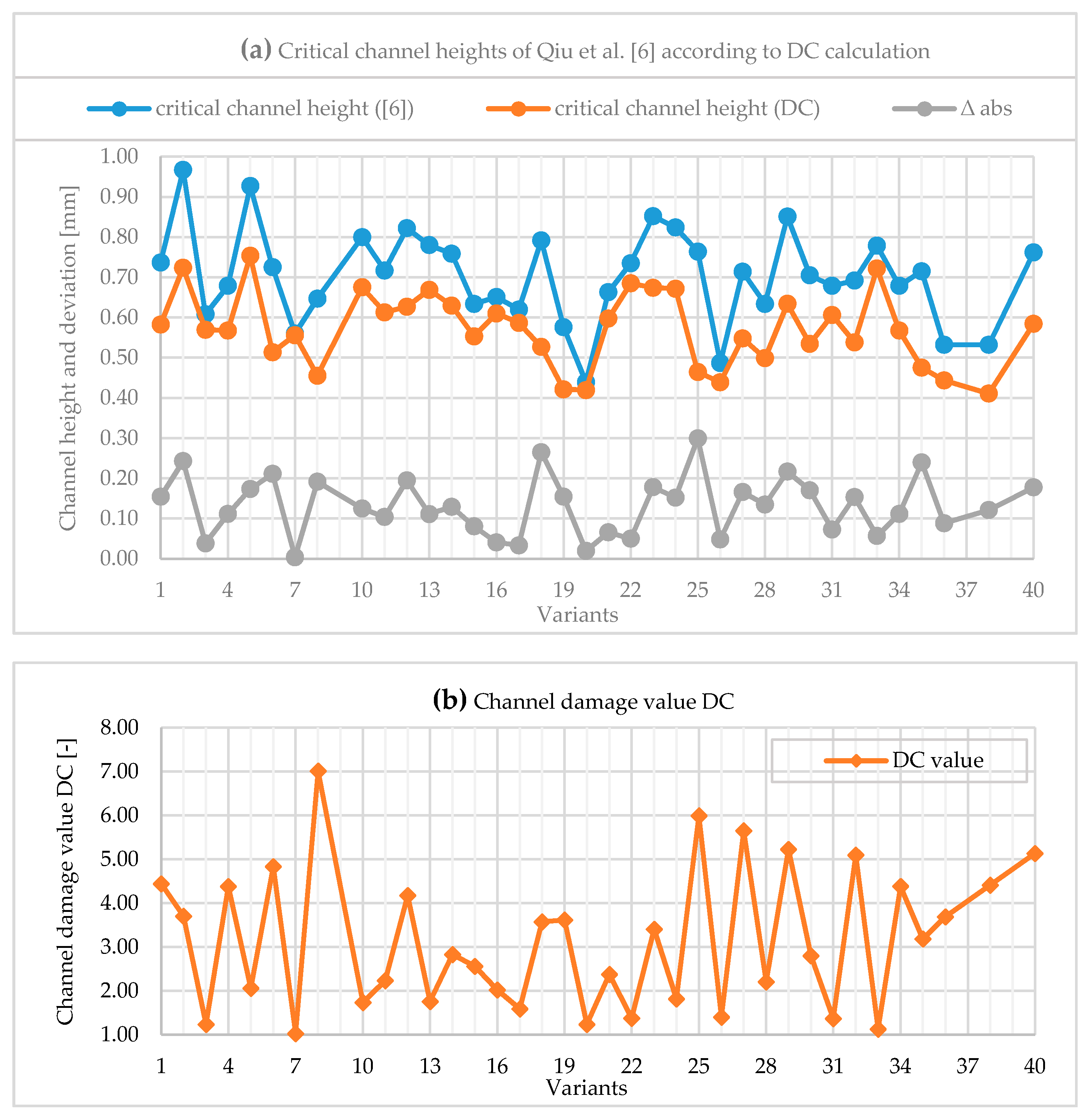
3.1. Comparison with the Results of Qiu et al. [6]

In [6], a total of 40 channel geometries were investigated experimentally. In each case, the forming experiments were carried out by means of mechanical deep drawing up to the first crack formation. Accordingly, a maximum achievable critical channel height results for each channel geometry. The respective channel parameters of all the variants can be taken directly from [6].

For the derived function Damage of Channel geometry (DC), the assumption is that the crack formation and thus, the destruction of the cross-sectional structure by a damage value of $DC=1$ is very probable. Accordingly, the damage value calculated from the channel parameters of each considered variant from [6] should ideally exceed this value, since it was always formed until the damage happens. Furthermore, by specifying the damage value to $DC=1$, the critical channel height can be determined by means of an appropriate retroactive calculation. The results with the critical channel heights of [6] and the calculated values according to DC calculation are shown below in Figure 8.

In the upper diagram (Figure 8a), it can be seen that the experimentally determined critical channel heights in each considered variant are higher than those calculated by DC. Thus, it can be determined with very high probability up to which critical channel height a channel cross-sectional contour can still be realized by forming. In addition, the qualitative behavior between the variants by comparison is calculable with good approximation. In particular, the statement about critical and less critical cross-sectional contours is thus also demonstrably possible by means of the DC calculation. On average, there is an error rate for the deviations of $18.20\%$ over all variants. The maximum deviation of $39.21\%$ is detected in variant 25, the minimum deviation of $6.33\%$ results from variant 7. For this experimental series, the high deviations can be considered as acceptable, because mechanical deep drawing up to the first crack formation will be investigated. In these cases, the assessment of the damage behavior based on DC calculation is more inaccurate. However, in such series of investigations, it is crucial that all variants can be determined as potentially critical variants ($DC\ge 1$) by means of DC calculation.

Furthermore, it can be seen, in the diagram below (Figure 8b), that for each variant, the calculated DC value is above the previously assumed limit value of $DC=1$. Consequently, after DC calculation, all variants are to be evaluated as likely critical and will probably lead to failure. From the point of view of the DC function application in an early development state, the results shown are evaluated as very positive. This implies that a comparatively simple assessment of the probability of damage of different cross-sectional structures in the qualitative range and partly also based on quantitative results is feasible.

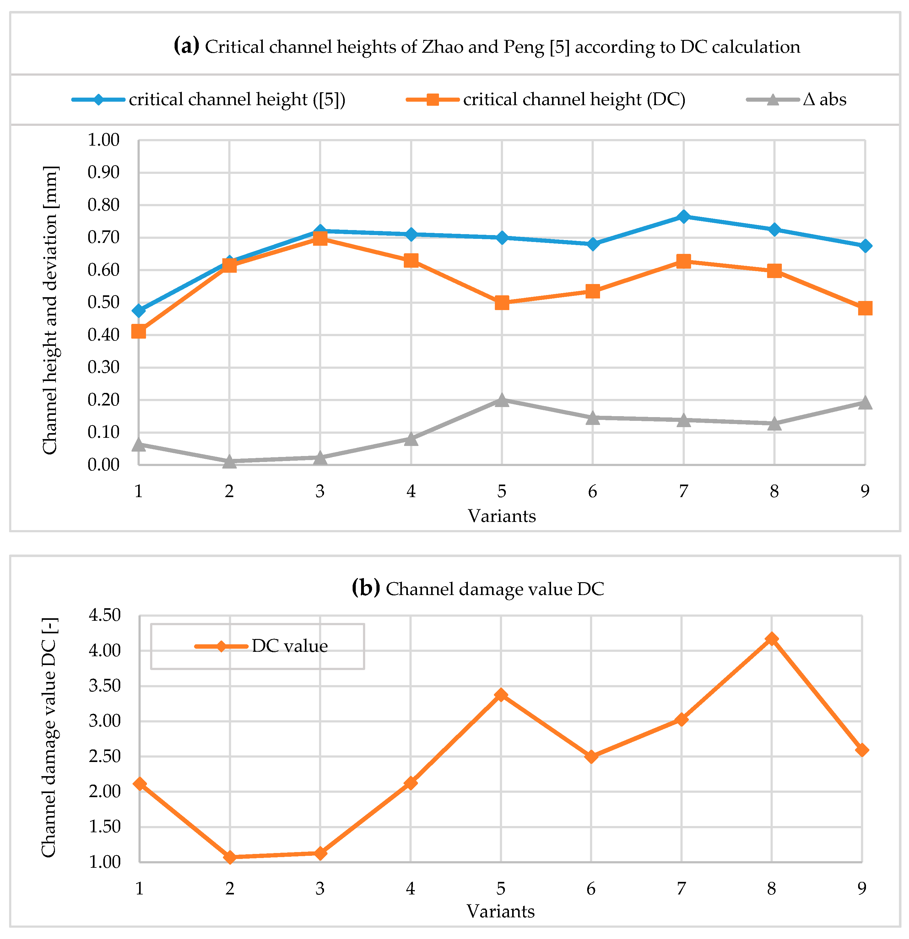
3.2. Comparison with the Results of Zhao and Peng [5]

In [5], a total of nine channel geometries were investigated experimentally. All other boundary conditions and requirements stood the same, as already explained for [6]. The respective channel parameters of all variants can be taken directly from the paper [5].

Regarding the calculation of the DC values and the critical channel heights, the same assumptions and boundary conditions apply as described in Section 3.1. In the following Figure 9, the results with the comparison of the critical channel heights and the results with the calculated DC values are shown.

It can be seen in the upper diagram (Figure 9a) that the experimentally determined critical channel heights in each considered variant are greater than those calculated by DC. The qualitative course between the calculation variants is again sufficiently mapped with only slight deviation. On average, there is an error rate for the deviations of $16.01\%$ regarding all variants. The maximum deviation of $28.69\%$ can be detected in variant 5 and the minimum deviation of $1.80\%$ is seen in variant 2. Regarding the calculation of the DC values and the relatively high deviations, the same assessments as described in Section 3.1 can be used here too.

Furthermore, in Figure 9b, it can also be seen that for the test series, each variant of the calculated DC value is above the previously assumed limit value of $DC=1$. All variants considered here will probably lead to mechanical failure.

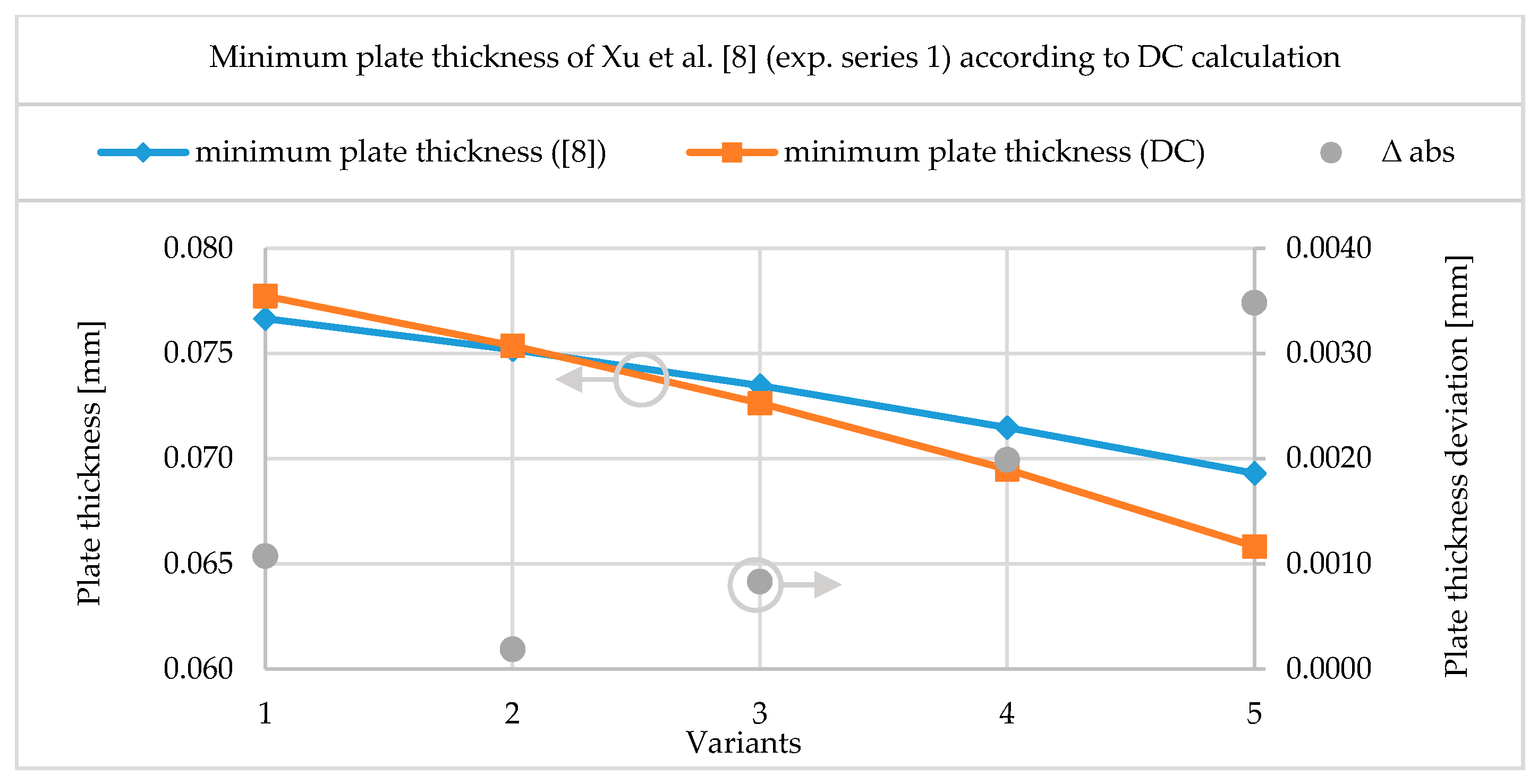
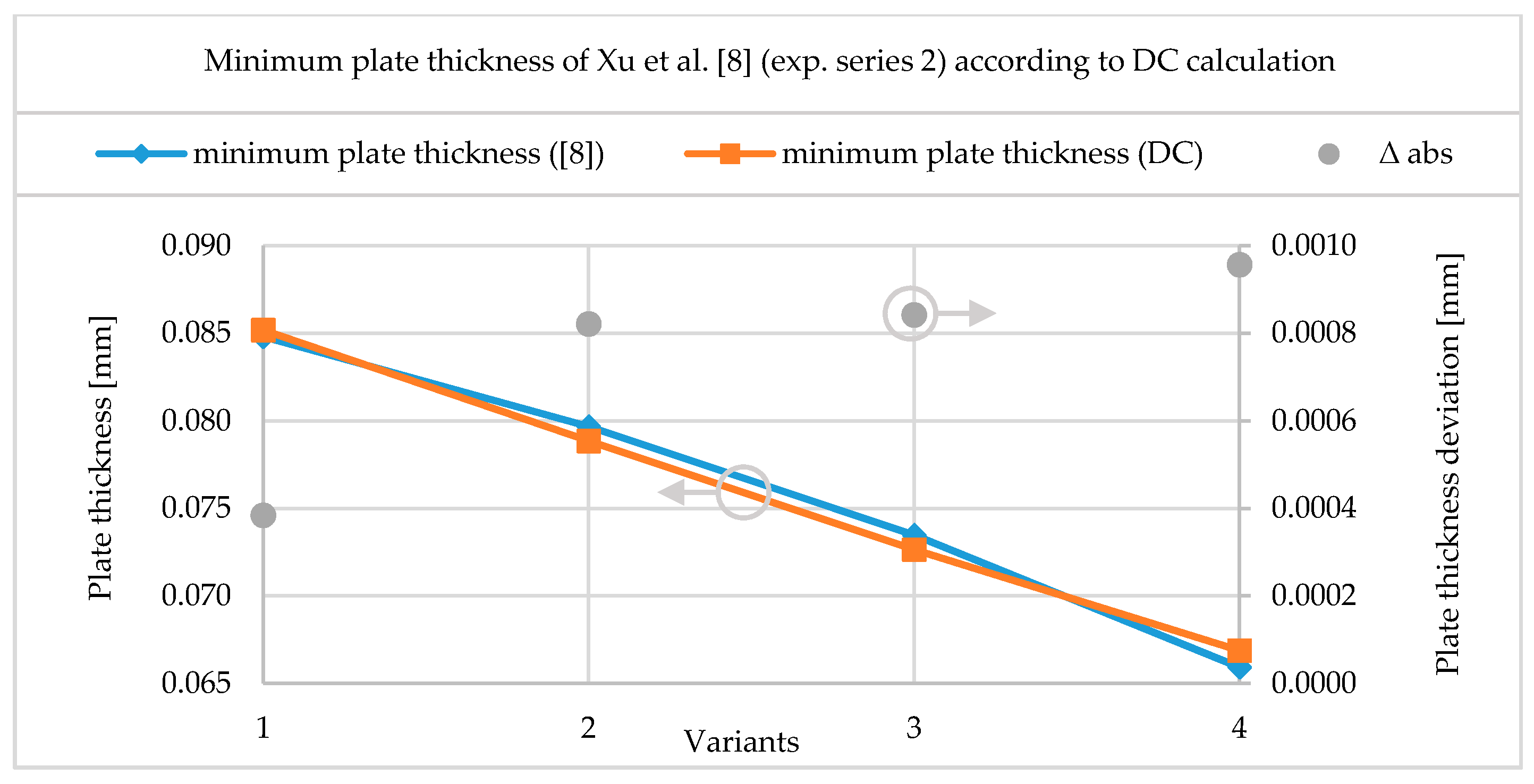
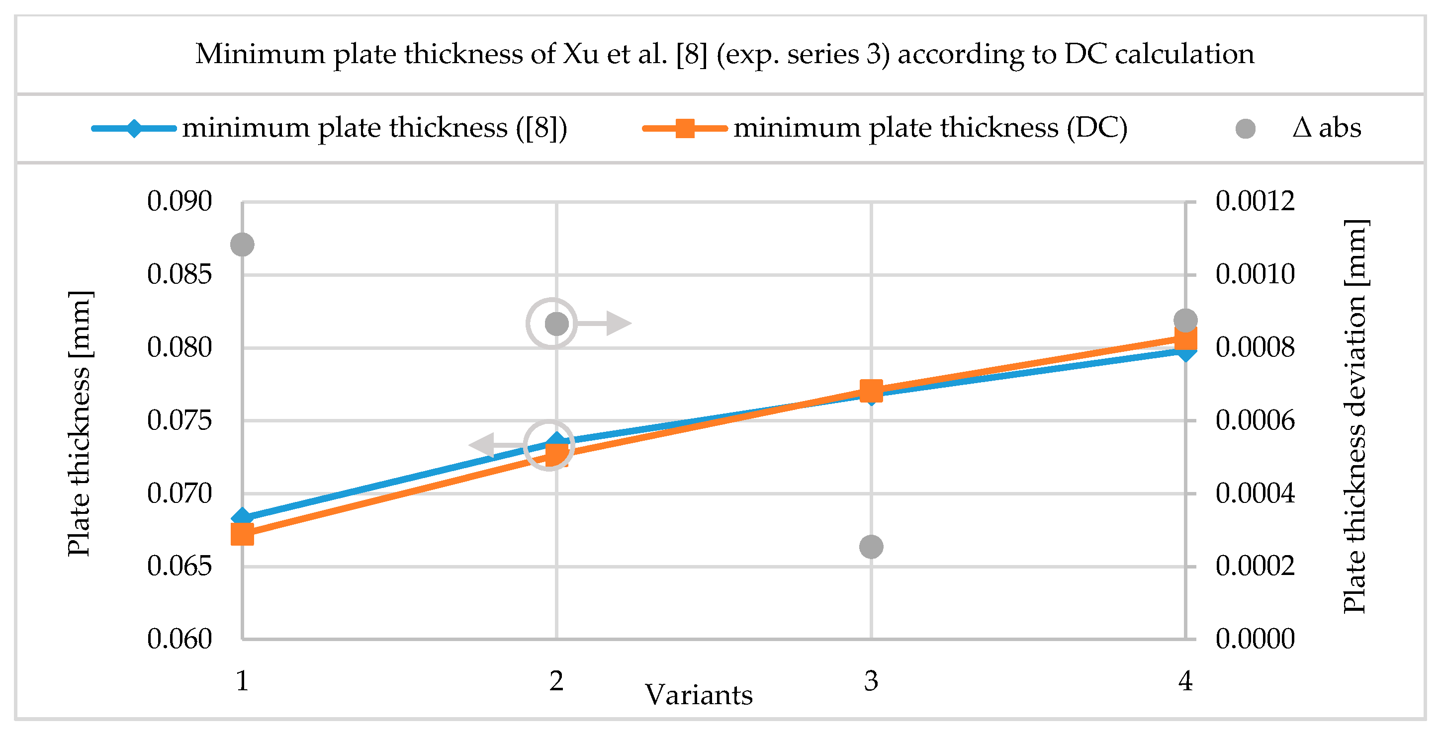
3.3. Comparison with the Results of Xu et al. [8]

As already mentioned in Section 1.1, the formability of channel structures in three test series, each with a different parameter, was carried out by means of a 2D FE Model approach in [8]. Respectively, the width of the punch on the upper die (five variants), the channel height (four variants) and the radii (four variants) were varied. In addition to the analysis of the occurring stresses, the minimum sheet thicknesses of the formed cross-sectional contours were determined. These are compared below with the minimum sheet thicknesses calculated according to DC.

Figure 10 shows the results of test series 1 for the variation of the width of the punch on the upper die. The increasing punch width always leads to steeper channel flank angles if the other channel parameters remain unchanged (variant 1: $CFA=44.55°$ → variant 5: $CFA=25.25°$). An analogously increasing sheet thinning is therefore plausible.

It can be seen that the qualitative and quantitative behaviors of both curves agree sufficiently well. The mean deviation of all variants is $2.12\%$, the maximum deviation of $5.02\%$ can be found in variant 5. This also represents the variant with the greatest sheet thinning. According to the DC calculation, the damage probability here is $DC=0.772$.

The following Figure 11 shows the results of test series 2 for the variation of the channel height. Analogously to test series 1, the increasing channel height per variant with otherwise constant geometry leads to a change in the channel flank angle—this also becomes steeper in this case. The increasing sheet thinning, therefore, meets the technical expectations.

It can be seen that the qualitative and quantitative behaviors of both curves correspond with good approximation. The average deviation over all variants is $1.02\%$ with a maximum deviation of $1.45\%$ found in variant 4. This also represents the variant with the highest sheet thinning. According to the DC calculation, the probability of damage hereby is $DC=0.842$.

Finally, in the following Figure 12, the results of the experimental series 3 for the variation of the radii (outside and inside radius) are shown. Unlike in the previous test series 1 and 2, the change of radii automatically varies other channel parameters. Basically, it is expected that with increasing radii, the resulting sheet thicknesses will increase analogously due to the low constricting tendency.

This assumption is confirmed not only in the results according to [8], but also in the values calculated by means of DC. Both curves are again sufficiently comparable in terms of quality and quantity. The average deviation over all variants is $1.05\%$, the maximum deviation of $1.59\%$ can be seen in variant 1. This also represents the variant with the greatest sheet thinning. According to the DC calculation, the damage probability is $DC=0.710$.

3.4. Comparison with the Results of Our Own FE Simulations

As already mentioned in Section 2.2, in addition to the comparisons with the results of other authors, validation experiments were carried out using our own 2D forming simulations. All of the numerical simulations are based on a calibrated model setup, which was shown and proved in Section 2.2.2. For this purpose, a total of 22 different channel cross-sectional structures were defined. Below is an overview of the range in which the channel parameters have been varied.

• channel width     $0.872\mathrm{mm}$ to $1.655\mathrm{mm}$
• channel ground   $0.100\mathrm{mm}$ to $0.500\mathrm{mm}$
• inner radius         $0.070\mathrm{mm}$ to $0.200\mathrm{mm}$
• outer radius         $0.170\mathrm{mm}$ to $0.300\mathrm{mm}$
• sheet thickness     $0.060\mathrm{mm}$ to $0.100\mathrm{mm}$
• channel height     $0.300\mathrm{mm}$ to $0.600\mathrm{mm}$

In Figure 13, the results of the simulations and DC calculations are compared. In the upper diagram Figure 13a, the maximum degree of deformation according to FEM simulation and the calculated damage value DC are compared. It becomes clear that both curves qualitatively and mostly quantitatively agree well. The average deviation over all 22 variants is $13.86\%$, a maximum deviation of $32.20\%$ can be found in variant 16, and the minimum deviation of $0.61\%$ results from variant 6.

Analogous evaluations and assessments can be seen in the lower diagram Figure 13b. There, the minimum sheet thicknesses according to FEM and DC calculation are shown comparatively. The average deviation is $7.53\%$, a maximum deviation of $18.20\%$ can be found in variant 22, the minimum deviation of $0.13\%$ results from variant 14.

4. Conclusions

In this work, an analytical calculation method for the estimation of the formability of channel cross section structures is presented. For this purpose, a general valid channel parameter definition is performed initially. In this framework, a universally usable equation is derived, which can be used in compliance with specified restrictions for the clear description of channel cross sections. Other definitions and approaches for the description of channel cross sections from literature can be used on the established equation.

Furthermore, an applied numerical 2D FE model for forming simulations is presented. The results obtained through the FE model were validated by experimental tests.

Subsequently, the derivation of the estimating function is listed. All influencing factors contained herein are explained and the overall DC function presented.

Finally, comparative considerations for the validation of the results from the DC calculation are carried out in comparison to the results from the listed technical literature. For the general applicability of the DC function and determined results, the following conclusions can be listed:

• The DC calculation method described above makes it possible to obtain an initial, fast and sufficiently accurate estimation regarding to the formability of channel cross section structures in an early development process and based on this, evaluate comparatively.
• Inaccuracies in the DC method can be detected, especially in variants with extreme geometry. In the calculations, the highest deviations appear mostly by variants with very small radii, small channel flank angles or large channel depths.
• To date, the DC calculation method has only been validated on forming results based on stainless steel sheets (e.g., SS304) with relatively homogeneous (in particular non-coarse grain structure) material properties. In addition, comparisons have only been made with sheet thicknesses between $0.060\mathrm{mm}$ and $0.100\mathrm{mm}$. The applicability to other materials and sheet thicknesses is to be assessed as realistic.
• In particular, when considering critical channel depths, a very good predictability has been demonstrated. At a value of $DC=1$ the experimentally determined critical channel depth has not been exceeded in any of the cases considered. This suggests that with the support of the DC Method, it can be at least stated, with a great probability, up to which limit depth a channel structure can still be safely formed.

Even the calculation of the sheet thinning by the DC-Model has, in most cases, a very good agreement with the given values from literature or our own experiments.

References

1. Kurzweil, P. Brennstoffzellentechnik: Grundlagen, Komponenten, Systeme, Anwendungen, 2nd ed.; Springer: Wiesbaden, Germany, 2013. [Google Scholar]
2. O’Hayre, R.P. Fuel Cell Fundamentals; John Wiley & Sons Inc.: Hoboken, NJ, USA, 2016. [Google Scholar]
3. Larminie, J.; Dicks, A. Fuel Cell Systems Explained, 2nd ed.; John Wiley & Sons Inc.: Hoboken, NJ, USA, 2011. [Google Scholar]
4. Peng, L.; Yi, P.; Lai, X. Design and manufacturing of stainless steel bipolar plates for proton exchange membrane fuel cells. Int. J. Hydrog. Energy 2014, 39, 21127–21153. [Google Scholar] [CrossRef]
5. Zhao, Y.; Peng, L. Formability and flow channel design for thin metallic bipolar plates in PEM fuel cells: Modeling. Int. J. Energy Res. 2018, 39, 21127. [Google Scholar] [CrossRef]
6. Qiu, D.; Peng, L.; Yi, P.; Lai, X.; Lehnert, W. Flow channel design for metallic bipolar plates in proton exchange membrane fuel cells: Experiments. Energy Convers. Manag. 2018, 174, 814–823. [Google Scholar] [CrossRef]
7. Hu, Q.; Zhang, D.; Fu, H. Effect of flow-field dimensions on the formability of Fe–Ni–Cr alloy as bipolar plate for PEM (proton exchange membrane) fuel cell. Energy 2015, 83, 156–163. [Google Scholar] [CrossRef]
8. Xu, S.; Li, K.; Wei, Y.; Jiang, W. Numerical investigation of formed residual stresses and the thickness of stainless steel bipolar plate in PEMFC. Int. J. Hydrog. Energy 2016, 41, 6855–6863. [Google Scholar] [CrossRef]
9. Khatir, F.A.; Elyasi, M.; Ghadikolaee, H.T.; Hosseinzadeh, M. Evaluation of Effective Parameters on Stamping of Metallic Bipolar Plates. Procedia Eng. 2017, 183, 322–329. [Google Scholar] [CrossRef]
10. Zhou, T.Y.; Chen, Y.S. Effect of Channel Geometry on Formability of 304 Stainless Steel Bipolar Plates for Fuel Cells—Simulation and Experiments. J. Fuel Cell Sci. Technol. 2015, 12, 51001. [Google Scholar] [CrossRef]
11. Bong, H.J.; Lee, J.; Kim, J.H.; Barlat, F.; Lee, M.G. Two-stage forming approach for manufacturing ferritic stainless steel bipolar plates in PEM fuel cell: Experiments and numerical simulations. Int. J. Hydrog. Energy 2017, 42, 6965–6977. [Google Scholar] [CrossRef]
12. Balali Osia, M. Forming Metallic Micro-Feature Bipolar Plates for Fuel Cell Using Combined Hydroforming and Stamping Processes. Iran. J. Energy Environ. 2013, 4, 91–98. [Google Scholar] [CrossRef]
13. Peng, L.; Hu, P.; Lai, X.; Ni, J. Fabrication of Metallic Bipolar Plates for Proton Exchange Membrane Fuel Cell by Flexible Forming Process-Numerical Simulations and Experiments. J. Fuel Cell Sci. Technol. 2010, 7, 31009. [Google Scholar] [CrossRef]
14. Elyasi, M.; Khatir, F.A.; Hosseinzadeh, M. Manufacturing metallic bipolar plate fuel cells through rubber pad forming process. Int. J. Adv. Manuf. Technol. 2017, 89, 3257–3269. [Google Scholar] [CrossRef]
15. Jin, C.K.; Lee, K.H.; Kang, C.G. Performance and characteristics of titanium nitride, chromium nitride, multi-coated stainless steel 304 bipolar plates fabricated through a rubber forming process. Int. J. Hydrog. Energy 2015, 40, 6681–6688. [Google Scholar] [CrossRef]
16. Manso, A.P.; Marzo, F.F.; Barranco, J.; Garikano, X.; Garmendia Mujika, M. Influence of geometric parameters of the flow fields on the performance of a PEM fuel cell. A review. Int. J. Hydrog. Energy 2012, 37, 15256–15287. [Google Scholar] [CrossRef]
17. Cooper, N.J.; Smith, T.; Santamaria, A.D.; Park, J.W. Experimental optimization of parallel and interdigitated PEMFC flow-field channel geometry. Int. J. Hydrog. Energy 2016, 41, 1213–1223. [Google Scholar] [CrossRef]
18. Manso, A.P.; Marzo, F.F.; Mujika, M.G.; Barranco, J.; Lorenzo, A. Numerical analysis of the influence of the channel cross-section aspect ratio on the performance of a PEM fuel cell with serpentine flow field design. Int. J. Hydrog. Energy 2011, 36, 6795–6808. [Google Scholar] [CrossRef]
19. Shimpalee, S.; vanZee, J.W. Numerical studies on rib & channel dimension of flow-field on PEMFC performance. Int. J. Hydrog. Energy 2007, 32, 842–856. [Google Scholar]
20. Ghanbarian, A.; Kermani, M.J.; Scholta, J.; Abdollahzadeh, M. Polymer electrolyte membrane fuel cell flow field design criteria—Application to parallel serpentine flow patterns. Energy Convers. Manag. 2018, 166, 281–296. [Google Scholar] [CrossRef] [Green Version]
21. Wang, X.D.; Huang, Y.X.; Cheng, C.H.; Jang, J.Y.; Lee, D.J.; Yan, W.M.; Su, A. Flow field optimization for proton exchange membrane fuel cells with varying channel heights and widths. Electrochim. Acta 2009, 54, 5522–5530. [Google Scholar] [CrossRef]
22. Yang, W.J.; Wang, H.Y.; Lee, D.H.; Kim, Y.B. Channel geometry optimization of a polymer electrolyte membrane fuel cell using genetic algorithm. Appl. Energy 2015, 146, 1–10. [Google Scholar] [CrossRef]
23. Zeng, X.; Ge, Y.; Shen, J.; Zeng, L.; Liu, Z.; Liu, W. The optimization of channels for a proton exchange membrane fuel cell applying genetic algorithm. Int. J. Heat Mass Transf. 2017, 105, 81–89. [Google Scholar] [CrossRef]
24. Kim, A.R.; Shin, S.; Um, S. Multidisciplinary approaches to metallic bipolar plate design with bypass flow fields through deformable gas diffusion media of polymer electrolyte fuel cells. Energy 2016, 106, 378–389. [Google Scholar] [CrossRef]
25. Breuer, J. Geometrische Einflüsse auf die strukturmechanische Belastbarkeit metallischer Bipolarplatten in PEM-Brennstoffzellen. Master’s Thesis, Technische Universität Chemnitz, Chemnitz, Germany, 2016. [Google Scholar]
26. Mohr, P. Optimierung von Brennstoffzellen-Bipolarplatten für die automobile Anwendung. Ph.D. Thesis, Universität Duisburg-Essen, Duisburg, Germany, 2018. [Google Scholar]
27. Keller, N.; von Unwerth, T. Rechnergestützte Synthese von Polymerelektrolyt-Membran-Brennstoffzellen. In Proceedings of the Fc³-1st Fuel Cell Conference Chemnitz 2019—Saubere Antriebe, Effizient Produziert, Saxony, Germany, 26–27 November 2019; pp. 172–181. [Google Scholar]
28. Bauer, A.; Härtel, S.; Awiszus, B. Manufacturing of Metallic Bipolar Plate Channels by Rolling. J. Manuf. Mater. Process. 2019, 3, 48. [Google Scholar] [CrossRef] [Green Version]
29. Bauer, A.; Graf, M.; Härtel, S.; Awiszus, B. Investigations on the optimization of the initial state for the forming process of metallic bipolar plates. In Proceedings of the Conference Speech: 21st International Conference on Advances in Materials & Processing Technologies, Dublin, Ireland, 2018. [Google Scholar]
Figure 1. Geometric relations of the forming dies (idealized contour).
Jmmp 04 00001 g001
Figure 2. Channel parameters (graphitic idealized—radii = 0 / CFA = 0°) [27].
Jmmp 04 00001 g002
Figure 3. Geometrical interrelations of channel parameters.
Jmmp 04 00001 g003
Figure 4. Channel forming 2D FEM setup.
Jmmp 04 00001 g004
Figure 5. Flow curve from bulge tests for 316 L (1.4404), thickness: 0.1 mm [28].
Jmmp 04 00001 g005
Figure 6. (a) Precision forming machine (P.FÜ.MA.) [29], (b) bipolar plate dummy (80 mm × 50 mm).
Jmmp 04 00001 g006
Figure 7. Comparison of the formed channel cross section between FEM (equivalent plastic strain) and experiment.
Jmmp 04 00001 g007
Figure 8. (a) Results of critical channel heights compared to DC; (b) Calculated DC values.
Jmmp 04 00001 g008
Figure 9. (a) Results of critical channel heights compared to DC; (b) calculated DC values.
Jmmp 04 00001 g009
Figure 10. Results of minimum plate thickness—experimental series 1.
Jmmp 04 00001 g010
Figure 11. Results of minimum plate thickness—experimental series 2.
Jmmp 04 00001 g011
Figure 12. Results of minimum plate thickness—experimental series 3.
Jmmp 04 00001 g012
Figure 13. (a) Maximum degree of deformation of FEM compared to DC; (b) Minimum plate thickness of FEM compared to DC.
Jmmp 04 00001 g013