Analytical Calculation of Cutting Forces in Ball-End Milling with Inclination Angle

Abstract

The traditional analytical cutting force prediction method for ball-end milling ignores the effect of the inclination angle on cutting forces. In this paper, a new experimental method for cutting force prediction methods considering the inclination angle in the ball-end milling process is proposed. First, the actual immersion ranges of cutter in the ball-end milling process with and without an inclination angle are analyzed by a geometrical method and the cutting force prediction model with an inclination angle is developed by a numerical integration method. Second, considering that entry and exit angles of cutting zones for different cutter layers vary due to the inclination angle, a milling force coefficients identification approach for different cutter layers is established by experimental calibration. Comparing the traditional analytical cutting force prediction method that ignores the inclination angle, the numerical simulation results show that the prediction force values calculated by the proposed method have a better consistency with the measured values.

1. Introduction

With normal vector self-adaptability, ball-end milling cutters are extensively used in machining parts with sculptured surfaces in the aerospace and motor industries [1,2,3] such as an aircraft engine blade, an integral impeller, and more. In the ball-end milling process, the contact interface between the cutter and work piece is constantly changing, which results in the changes of the cutting force, cutter wear state, vibration, machining precision, and more. Cutting force modeling is the basis of modeling and analysis of ball end cutter milling process especially for a milling process analysis and cutting force prediction. To solve this problem, most scholars mainly analyze the cutting process based on shear angle theory and friction angle theory combined with oblique cutting and orthogonal cutting models. Jain and Yang [4,5] calculated a cutting force based on cutting force data in a Cartesian coordinate system. Feng et al. [6,7] established a nonlinear local cutting force model in the form of power function based on an approximate cutting edge equation and gave a cutting force model of ball-end milling cutter with runout. Lee and Altintas [8] adopted a spherical spiral line geometric model and decomposed the cutting force on oblique cutting edge segments using the oblique cutting model by considering a ploughing force. Yucesan and Altintas [9] analyzed the spherical geometric characteristics of the ball-end cutting edge and calculated the cutting force through pressure and friction forces on the rake face and flank face of the cutter. However, the above analytical models do not analyze the cutting state in which there is an inclination angle between the cutter axis and work piece surface. In a practical process, an inclination angle is often used in order to avoid zero cutting speed at the tip of the ball. Additionally, the inclination angle has a significant influence on machined surface quality and process efficiency. In order to improve the milling process, some researchers [10,11] focus on minimizing cutting forces and vibrations by adjusting the inclination angle. Ultimately, the milling quality is boiled down to cutting forces and its components. Therefore, cutting forces prediction is key for improving the milling process.

For the cutting force prediction, the precise calculation of the cutting zone is particularly important for the analysis of the cutting process and force calculation. In this paper, a cutting force computational model based on the Altintas [12] milling force model is proposed by analyzing cutter entry and exit angles of cutting elements in different cutting states and validity of the model is verified by simulation and experiment.

2. Modeling of Ball-End Milling Force

2.1. Geometric Model of Ball End Milling Cutter

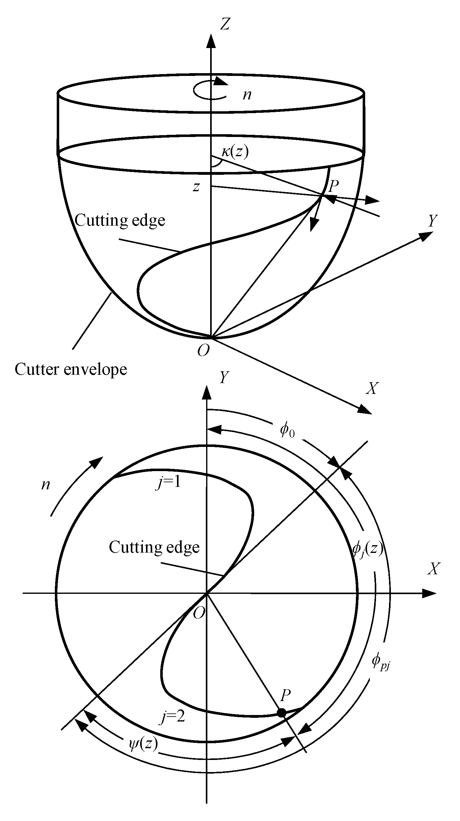
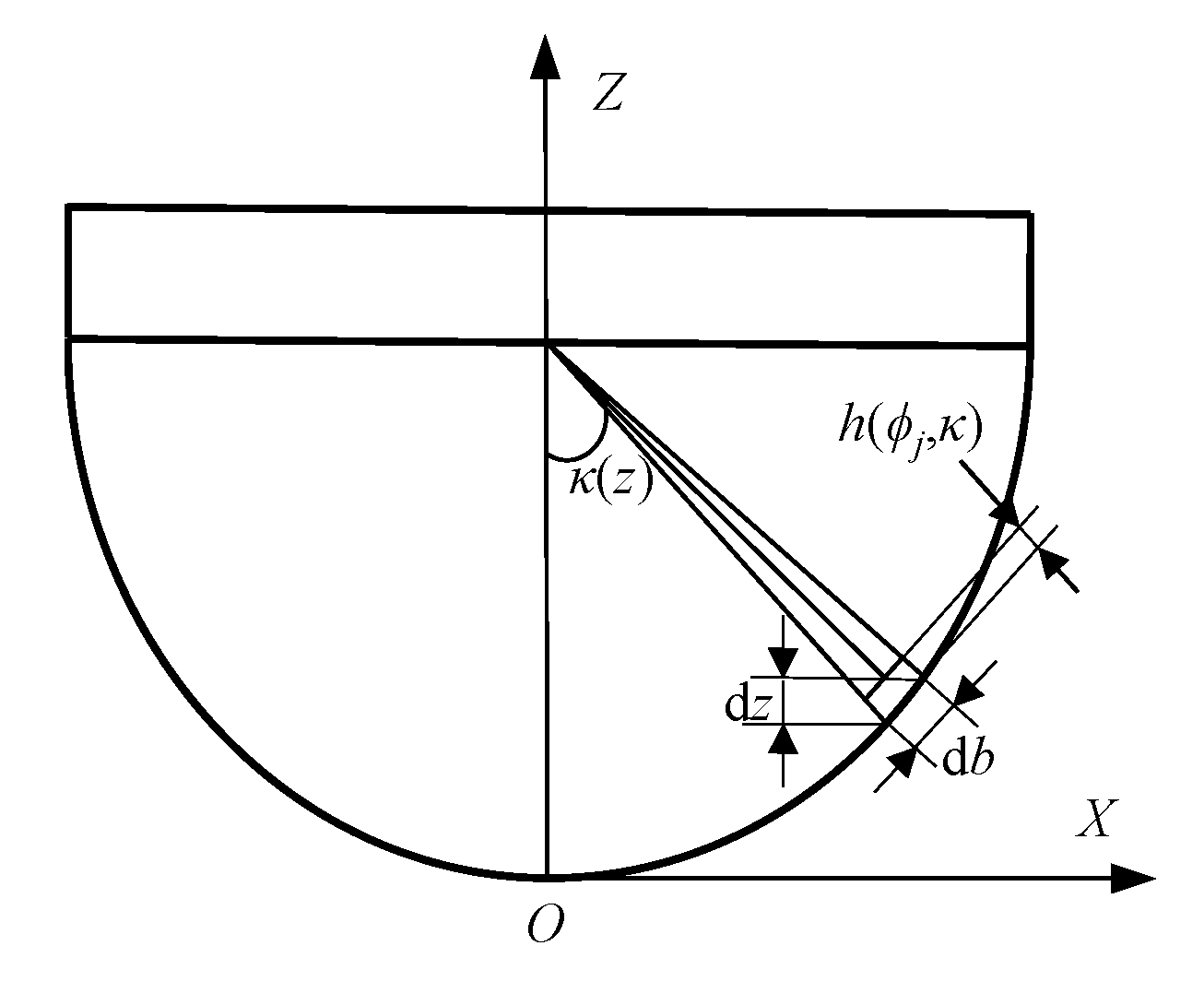
The geometry of the cutting edge of a ball-end milling cutter is shown in Figure 1. The cutting edges meet at the tip of the ball and are rising along the axis of the cutter with a constant helix lead. Cutter elements are obtained by splicing the cutter into slices along the horizontal direction and the corresponding cutting position is approximately assumed to be the middle point of the cutter element. Assuming point P is at the middle position of one cutter element at the height of z (the height is along cutter axis relative to point O on the tip of the ball part and, if no specific explanation, the following is the same), so differential cutting force at point P can be decomposed into three components dF_t, dF and dF_a. The cutter radius r(z), the rotation lag angle ψ(z), and the axial immersion angle κ(z) of point P are important parameters for identifying the cutting force. The cutter radius r(z) denotes the radius of the circle in the XY plane at point P. The rotation lag angle ψ(z) is the angle between the tangent line of the cutting edge and line OP in the XY plane. The axial immersion angle κ(z) is the angle between the cutter axis and normal vector of point P. In practical processes, the ball part of the cutter is mainly used for cutting, which means only the ball part of the cutter is considered.

The vector from point O to any point on the spiral cutting edge is expressed by the equation below.

$$\overrightarrow{r}=x_j\overrightarrow{i}+y_j\overrightarrow{j}+z_j\overrightarrow{k}=r({\varphi }_j)(\sin {\varphi }_j\overrightarrow{i}+\cos {\varphi }_j\overrightarrow{j})+z({\varphi }_j)\overrightarrow{k},$$

(1)

where ${\varphi }_j$ can be written in terms of the rotation angle and lag angle ψ(z) and cutter pitch angle is the radial immersion angle of point P on the j-th cutting edge. Cutter radius r(z) can be expressed by the equation below.

$$r(z)=\sqrt{2Rz-z^2},$$

(2)

where R is radius of the ball part.

Taking the first cutting edge as the basic cutting edge and setting rotation angle at point O as ${\varphi }_0$, the radial immersion angle can be expressed by the equation below.

$${\varphi }_j(z)={\varphi }_0+{\displaystyle \sum _{n=1}^j{\varphi }_{pj}}-\psi (z),$$

(3)

where ${\varphi }_{pj}$ is the cutter pitch angle. The lag angle is due to the helix angle. The differential length of the cutting edge is represented in the equation below.

$$\mathrm{d}S=\left|\mathrm{d}r\right|=\sqrt{r^2({\varphi }_j)+{(r^{\prime }({\varphi }_j))}^2+{(z^{\prime }({\varphi }_j))}^2}\mathrm{d}\varphi ,$$

(4)

and unreformed chip thickness can be approximated in terms of as ${\varphi }_j$ and $\kappa$:

$$h({\varphi }_j,\kappa )=s_t\sin {\varphi }_j\sin \kappa ,$$

(5)

where $s_t$ is the feed rate (mm/tooth).

2.2. Modeling of Cutting Force

The tangential $\left(\mathrm{d}{F}_t\right)$, radial $\left(\mathrm{d}{F}_r\right)$ and axial $\left(\mathrm{d}{F}_a\right)$ cutting forces acting on the differential cutting edge given by Altintas [10] are determined by the formulas below.

$$\begin{array}{l}\mathrm{d}{F}_t=K_{te}\mathrm{d}S+K_{tc}h({\varphi }_j,\kappa )\mathrm{d}b\\ \mathrm{d}{F}_r=K_{re}\mathrm{d}S+K_{rc}h({\varphi }_j,\kappa )\mathrm{d}b\\ \mathrm{d}{F}_a=K_{ae}\mathrm{d}S+K_{ac}h({\varphi }_j,\kappa )\mathrm{d}b\end{array},$$

(6)

where the subscript c and e denote cutting and edge force components, respectively. Edge force coefficients $K_{te}$, $K_{re}$ and $K_{ae}$ are constant and cutting force coefficients can be calculated by slot milling tests or by orthogonal-to-oblique transformation given by Budak [13]. Chip width $\mathrm{d}b=\mathrm{d}z/\sin \kappa (z)$ is defined as the length of the tangent line of the cutting envelope for a differential axial length, which was illustrated in Figure 2. The chip thickness is estimated by using the kinematics theory of milling and the vibration of both the cutter and the workpiece.

Assuming the spindle speed and feed rate are constant, the tangential, radial, and axial forces are transformed into cutter Cartesian coordinates that consider a transformation in terms of the axial and radial immersion angle.

$$\left[\begin{array}{l}\mathrm{d}{F}_x\\ \mathrm{d}{F}_y\\ \mathrm{d}{F}_z\end{array}\right]=\left[\begin{array}{ccc}-\cos {\varphi }_j& -\sin {\varphi }_j\sin \kappa & -\sin {\varphi }_j\cos \kappa \\ \sin {\varphi }_j& -\cos {\varphi }_j\sin \kappa & -\cos {\varphi }_j\cos \kappa \\ 0& -\cos \kappa & -\sin \kappa \end{array}\right]\left[\begin{array}{c}\mathrm{d}{F}_t\\ \mathrm{d}{F}_r\\ \mathrm{d}{F}_a\end{array}\right].$$

(7)

3. Effect of Inclination Angle on Cutting Force

The cutter is discretized into infinitesimal segments along the cutter axis and it is noted that cutting forces aren’t zero only when the cutting edge is in the cutting zone, i.e., the radial immersion angle is located between entry and exit angles. Afterward, the cutting forces are obtained by adding the forces of all segments.

Based on the above, it is concluded that cutting force calculation is on the level of the precise cutting zone. Without an inclination angle, entry and exit angles are the same for each axial segment. When there is an inclination angle between the cutter axis and workpiece surface, entry and exit angles are diverse. Entry and exit angles in two different cases will be further discussed.

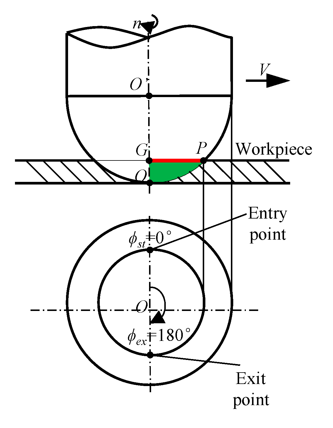
3.1. Without Inclination Angle

The schematic diagram of the milling process in this case is illustrated in Figure 3. Point O is the tip of the ball part and point O’ is the center of the ball part. The axial cutting depth is the length of line segment GO and point G, which is on the cutter axis, has a height equal to the axial cutting depth. The valid cutting zone is shown as the green zone GOP where point P is the intersection point of the cutting edge and work piece surface. GP stands for the highest axial segment of the cutter and only segments below GP participate in cutting. In this case, each segment has the same entry and exit angles, i.e., entry angle ${\varphi }_{\mathrm{st}}=0°$ and exit angle ${\varphi }_{\mathrm{ex}}=180°$.

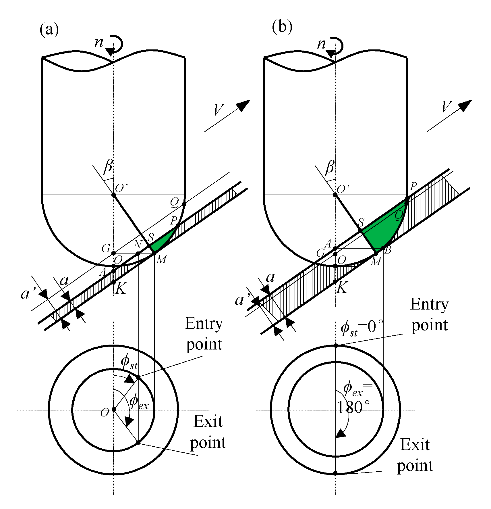
3.2. With Inclination Angle

When the axis of the cutter is tilted to the workpiece surface with a β inclination angle, the contact state between the cutter and the workpiece is shown in Figure 4.

In Figure 4a, the cutter axis is tilted to the work piece surface with a β inclination angle. Additionally, the direction is parallel to the work piece surface. The cutting depth is the length of line segment SM. Point A is the intersection point of the cutter axis and work piece surface and the height of point A. $z_A$ is represented by the equation below.

$$z_A=\frac{a}{\cos \beta }-(\frac{R}{\cos \beta }-R).$$

(8)

The valid cutting zone is shown as the green zone SMP. Point G, which is on the cutter axis has an equal height with point M. The height of point M, $z_M$ is shown below.

$$z_M=R(1-\cos \beta ).$$

(9)

Point N is the intersection point of line segment GM and work piece surface. Entry and exit points of the cutter segment at the height of $z_M$ can be obtained by intersecting the circle with a vertical line through point N. Point P is the intersection point of the cutter envelope and work piece surface where entry and exit points coincide. Therefore, the cutter segments between point M and point P participate in cutting.

As the axial cutting depth increases, the distance between point A and point G decreases until the two points coincide. When the two points coincide, the cutting depth is represented below.

$$a^{\prime }=R{\sin }^2\beta .$$

(10)

When the axial cutting depth a ≤ a’, the cutting range scaled by the angle decreases as the height of the cutter segment between point M and point P increases. If the axial height of the cutter segment is z, the entry and exit angles of the cutter segment are expressed below.

$$\begin{array}{l}{\varphi }_{st}=\arcsin (\frac{z+z_O-z_A}{\tan \beta \cdot r(z)})\\ {\varphi }_{ex}=\pi -{\varphi }_{st}\end{array},$$

(11)

where

$$z_O-z_A=r(z_M)\tan \beta -\frac{a}{\cos \beta }-R(1-\cos \beta ).$$

(12)

When the axial cutting depth a > a´, the cutting state is shown as Figure 4b. The valid cutting zone is shown as the green zone SMP where point P is the intersection point of the cutting edge and work piece surface. Point B, which is on the cutter envelope, has an equal height with point A. The cutter segments between point M and point B have an entry angle =0° and an exit angle =180°. Entry and exit angles of other cutter segments are calculated by using Equation (11).

4. Milling Force Coefficients Identification

Janez G [14] proposed a method of cutting and edge force coefficients identification based on average edge forces related to cutter geometry and engagement of cutter and the work piece. For a cutter with given geometry, the cutting and edge coefficients in Equation (6) are obtained by equating the measured cutting forces with the corresponding analytical expressions. Given the cutter geometry and cutting parameters, the average cutting force per tooth at a specific feed rate is measured by a three-component dynamometer. Assuming linear dependence of the average force on the feed rate, the average force is estimated using linear regression for the feed rate. Then the relationship of cutting force between feed rate is identified by a least squares fit. Therefore, cutting and edge coefficients at different cutting conditions are obtained by decomposing cutting forces into cutting and edge forces. For each axial cutting depth, the feed rate needs to be changed in order to solve the linear regression of the cutting force to the feed rate, which causes a large workload. Moreover, for cutter with a complex shape, it is difficult to obtain accurate cutter geometry and the approximate cutter geometry will inevitably decrease the accuracy of the cutting force model.

In order to decrease the experiment times, a non-separate-edge force model is adopted in this paper, i.e., milling force components (tangential, radial, and axial) can be expressed as a product form of the milling force coefficient and chip load. For each milling force component, the shear effect of chip formation on the rake face and the ploughing effect on the cutting edge and rake face are expressed in the form of a milling force coefficient in which the chip load is the product of the instantaneous under-formed chip thickness and the cutting width. Three milling force components is defined below.

$$\{\begin{array}{l}{F}_{t,j}({\varphi }_j,\kappa )=K_{t}h({\varphi }_j,\kappa )\mathrm{d}b\\ F_{r,j}({\varphi }_j,\kappa )=K_{r}h({\varphi }_j,\kappa )\mathrm{d}b\\ F_{a,j}({\varphi }_j,\kappa )=K_{a}h({\varphi }_j,\kappa )\mathrm{d}b\end{array},$$

(13)

where K_t, K_r and K_a denote corresponding cutting coefficients. The instantaneous cutting forces at an immersion angle $\varphi$ are shown below.

$$\left[\begin{array}{c}{F}_x(\varphi )\\ F_y(\varphi )\\ F_z(\varphi )\end{array}\right]=\frac{f_z}{2}\left[\begin{array}{ccc}-K_t\sin 2\varphi & -2K_r{\sin }^2\varphi & -2K_a{\sin }^2\varphi \\ 2K_t{\sin }^2\varphi & -K_r\sin 2\varphi & -K_a\sin 2\varphi \\ 0& -2K_a\sin \varphi & 2K_r\sin \varphi \end{array}\right]\left[\begin{array}{c}{A}_1\\ A_2\\ A_3\end{array}\right],$$

(14)

where f_z is feed per tooth and A₁, A₂, and A₃ are cutter geometry and can be expressed by the equations below.

$$\begin{array}{l}{A}_1={z|}_{z_1}^{z_2},A_2={-\frac{R_c}{2}(E\sqrt{1-E^2}+\arcsin E)|}_{z_1}^{z_2}\\ A_3={\frac{1}{R_c}(r_{z}z-\frac{z^2}{2})|}_{z_1}^{z_2}\end{array},$$

(15)

where E(z) equates (r_z-z)/R. In this method, the cutting forces in the cutting zone are considered an equivalent load on the single cutter tooth and the corresponding cutting force coefficient is calculated below.

$$\begin{array}{l}\left[\begin{array}{c}{K}_t\\ K_r\\ K_a\end{array}\right]=\frac{2\pi }{f_z{N}_f}\cdot \\ \left[\begin{array}{ccc}\frac{1}{A_1}\cdot \frac{D_2}{D_2^2+D_1^2}& -\frac{1}{A_1}\cdot \frac{D_1}{D_2^2+D_1^2}& 0\\ \frac{A_2}{(A_2^2+A_3^2)}\cdot \frac{D_3}{D_2^2+D_1^2}& \frac{A_2}{(A_2^2+A_3^2)}\cdot \frac{D_2}{D_2^2+D_1^2}& -\frac{A_3}{(A_2^2+A_3^2)}\cdot \frac{1}{D_4}\\ \frac{A_3}{(A_2^2+A_3^2)}\cdot \frac{D_3}{D_2^2+D_1^2}& \frac{A_3}{(A_2^2+A_3^2)}\cdot \frac{D_2}{D_2^2+D_1^2}& \frac{A_2}{(A_2^2+A_3^2)}\cdot \frac{1}{D_4}\end{array}\right]\left[\begin{array}{c}{\overline{F}}_x\\ {\overline{F}}_y\\ {\overline{F}}_z\end{array}\right]\end{array}$$

(16)

where D₁, D₂, D₃ and D₄ are immersion constants shown below.

$$D=\left(D_1=(\frac{1}{4}{\sin 2\varphi -\frac{1}{2}\varphi )|}_{{\varphi }_{st}}^{{\varphi }_{ex}},D_2={\sin \varphi |}_{{\varphi }_{st}}^{{\varphi }_{ex}},D_3={\cos \varphi |}_{{\varphi }_{st}}^{{\varphi }_{ex}}\right).$$

(17)

The cutting force coefficients of each layer of the ball end milling cutter is identified. The solutions are shown in the following steps.

• Measure and obtain average cutting forces at a series of axial depth by experiment ${\overline{F}}_j,j=1,2,\cdots ,N$.
• The average cutting force of each cutter layer is obtained by solving the average cutting force difference between two adjacent axial cutting depths ${\overline{F}}_{Fj}={\overline{F}}_j-{\overline{F}}_{j-1}$.
• Substitute ${\overline{F}}_{Fj}$ into Equation (16) and the cutting force coefficients of each cutter layer are obtained.

The cutting coefficients are identified from standard slot milling experiments. The main cutting parameters and tool parameters used in the experiments are shown in

Table 1. Main cutting parameters and tool parameters.

Parameter	Spindle Speed (rpm)	Feed Rate (mm/min)	Helix Angle (°)	Cutter Radius (mm)	Cutter Flute
value	2500	320	35	5	2

. A total of six groups of experiments are carried out and the axial depth are 0.5 mm, 1 mm, 1.5 mm, 2 mm, 2.5 mm and 3 mm, respectively.

With this method, it is worth noting that the force coefficients for each cutter layer are at different axial heights z. The average cutting forces of one cutter tooth at different axial depths are shown in

Table 2. Average cutting forces of ball-end milling at different axial depths.

dp/mm	${\overline{\mathit{F}}}_{\mathit{x}}/\mathbf{N}$	${\overline{\mathit{F}}}_{\mathit{y}}/\mathbf{N}$	${\overline{\mathit{F}}}_{\mathbf{z}}/\mathit{N}$
0.5	−15.98	53.13	64.26
1	−19.46	38.10	30.29
1.5	−18.51	37.67	16.80
2	−25.23	36.17	11.70
2.5	−24.53	37.07	9.23
3	−23.07	36.84	−1.21

.

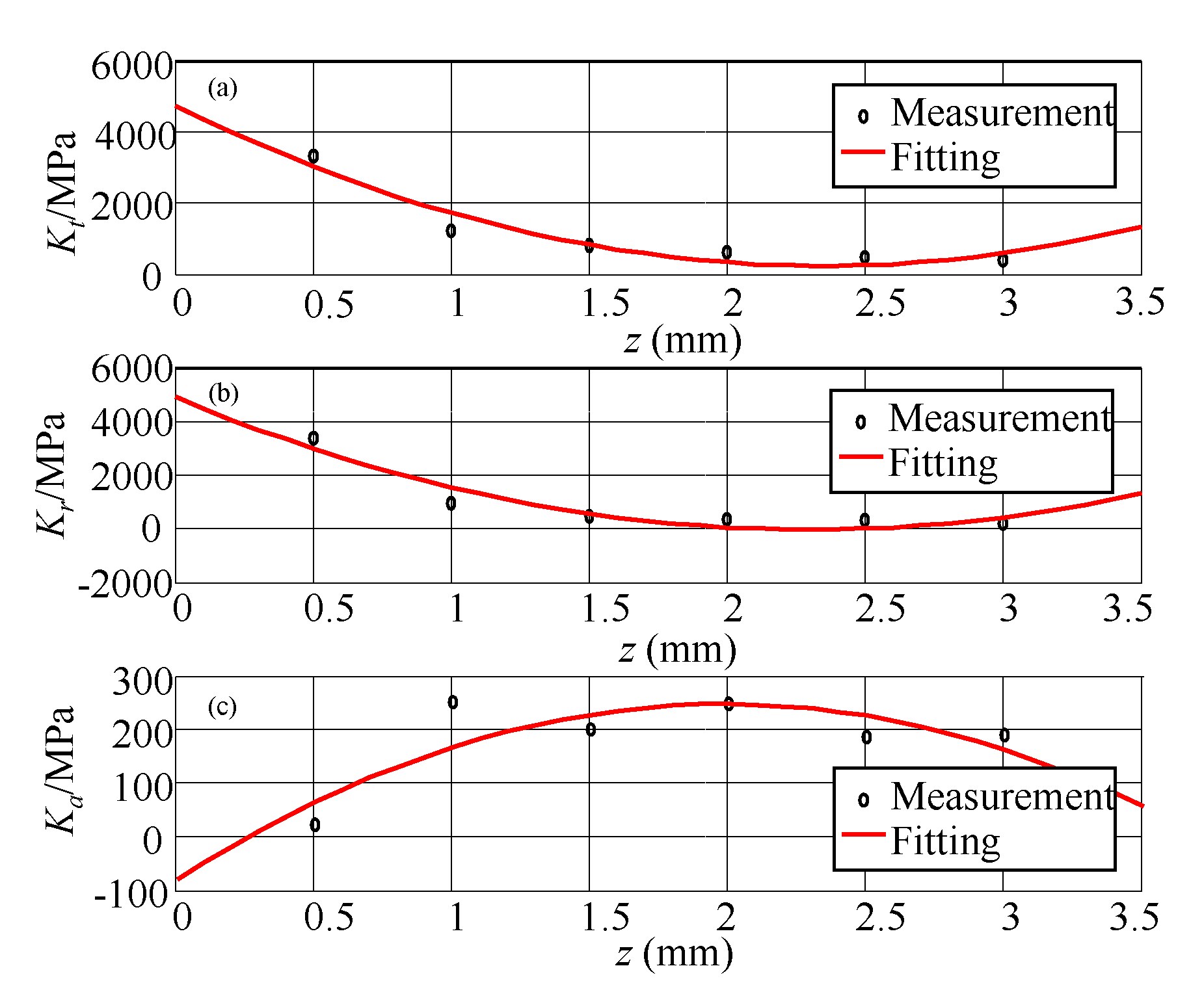
Substitute average cutting forces ${\overline{F}}_x$, ${\overline{F}}_y$ and ${\overline{F}}_z$ into Equation (16) and the corresponding cutting coefficients are obtained. The quadratic fitting curves of axial depth to cutting force coefficient curves are shown in Figure 5.

The expression of the force cutting coefficient in the quadratic fitting form of axial height z is shown below.

$$\{\begin{array}{l}{K}_t=817.8z^2-3838z+4735\\ K_r=934.3z^2-4293z+4886\\ K_a=-82.93z^2+329.3z-79.92\end{array}.$$

(18)

So far, the model of the cutting force coefficient on the axial cutting depth of the ball end milling is obtained.

5. Experimental Verification and Analysis

In order to verify the proposed cutting force prediction model above, verification tests are conducted and test conditions are listed in

Table 3. Test condition.

Workpiece Material	Titanium alloy TC4
Ball-End Milling Cutter	Material: cemented carbide, two flutes, radius: 10 mm
Experimental Equipment	CNC machining center: YHVT850Z
	Three-component Dynamometer: Kistler 9255B
	charge-amplifier: Kistler 5019B
	Data acquisition equipment: DEWE3010
Cutting Parameter	Spindle speed: 2500 rpm Feed rate: 320 mm/min Cutting depth: 2 mm Inclination Angle: 15°, 25°

.

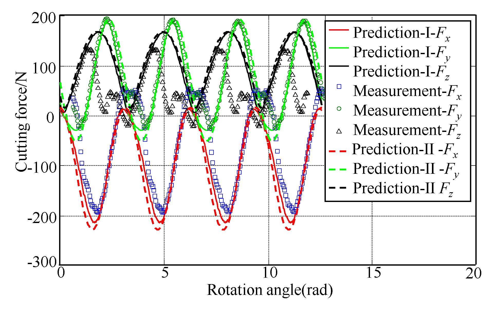
The work piece is clamped with a specific inclination angle by a vice and the whole device is clamped on the dynamometer. The measured and predicted cutting forces are shown in Figure 6 and Figure 7. F_x is the feed force and F_z is the cutting force along the tool axis direction.

The spindle runout has an effect on the curve of measured cutting forces in practical milling experiments, which causes the adjacent waves to be diverse. In Figure 6 and Figure 7, this effect has been eliminated by data processing, e.g., the cutting force during one spindle period is the mean force of cutting forces during different tooth periods.

Figure 6 and Figure 7 show measured and predicted forces with inclination angles 15° and 25°, respectively. In the figures, alternate ‘Prediction-I’ (solid line) denotes the predicted cutting forces using the method proposed in this paper and alternate ‘Prediction-II’ (dash line) denotes the predicted cutting forces without considering the change of immersion ranges with the change of height of the cutter layer due to inclination angles. It can be observed that the predicted cutting forces using the method proposed in this paper correspond better with measured cutting forces. The cutting force in the z-direction is affected by the material flow on the cutting edge ignored in the model and causes discrepancy.

6. Conclusions

Comparing two cutting situations in ball-end milling process, the cutter axis is perpendicular to the workpiece surface and the other cutter axis is tilted to the workpiece surface. The motion of the ball end milling cutter is analyzed. The actual immersion ranges of cutter and contact interface between cutter and workpiece are obtained.

Due to the inclination angle, the immersion ranges of cutter layer changes with the height of the cutter layer and entry and exit angles of each cutter layer are calculated. In order to obtain cutting coefficients, the average cutting force of each cutter layer is obtained by solving the average cutting force difference between two adjacent axial cutting depths and the cutting force coefficients of each cutter layer are obtained. It is worth noting that the cutting force coefficient obtained is not the function of the axial cutting depth but is the function of the height of the cutter layer.

By experimental verification, predicted cutting forces using the proposed method, which considers entry and exit angles of each cutter layer, correspond better with measured cutting forces. Without considering entry and exit angles changing, the prediction cutting force in the feeding direction has a larger error with measured forces than the other two directions.

When the axis of ball-end milling cutter is tilted to the workpiece surface, the axial cutting depth and the radial cutting width of the ball-end milling cutter are difficult to distinguish especially in the case of the small cutting depth. The cutting depth criteria based on the cutter cannot accurately reflect the actual depth of cutting. In this paper, the actual cutting depth of the work piece is transformed into the axial cutting depth of the cutter. Traditional analytical cutting force prediction method turns cutters into discrete layers along the tool axis, which is more accurate when the tool axis is perpendicular to the workpiece surface. While the tool axis is tilted, the immersion range of each cutter layer is different. In this paper, a formula for calculating the entry and exit cutting angles of the cutter layer considering axial height is put forward. Cutting force coefficients of different cutter layers are calibrated and the accuracy of the cutting force prediction improves.