Abstract
This study introduces an innovative refinement to EKF-based monocular SLAM by incorporating attitude, altitude, and range-to-base data to enhance system observability and minimize drift. In particular, by utilizing a single range measurement relative to a fixed reference point, the method enables unmanned aerial vehicles (UAVs) to mitigate error accumulation, preserve map consistency, and operate reliably in environments without GPS. This integration facilitates sustained autonomous navigation with estimation error remaining bounded over extended trajectories. Theoretical validation is provided through a nonlinear observability analysis, highlighting the general benefits of integrating range data into the SLAM framework. The system’s performance is evaluated through both virtual experiments and real-world flight data. The real-data experiments confirm the practical relevance of the approach and its ability to improve estimation accuracy in realistic scenarios.
1. Introduction
Navigating unmanned aerial vehicles (UAVs) in GPS-denied environments remains a complex challenge in robotics, where high precision and robustness are crucial for autonomous operations. Applications such as search and rescue, environmental monitoring, and infrastructure inspection increasingly require reliable localization and mapping solutions under such constraints. When GPS is unavailable or unreliable, Simultaneous Localization and Mapping (SLAM) serves as a key enabler for real-time navigation autonomy. Among SLAM methods, monocular SLAM (MonoSLAM) is widely utilized due to its lightweight nature and compatibility with UAV platforms. However, MonoSLAM is inherently limited by scale ambiguity, depth estimation challenges, and cumulative drift, which worsen over time in complex environments.
Recent advancements in visual SLAM have significantly improved performance. Systems like ORB-SLAM [1] and its successor ORB-SLAM3 [2] provide robust solutions for monocular-based navigation in large-scale environments. ORB-SLAM3 introduces multi-map capabilities and integrates inertial measurement unit (IMU) data, enhancing adaptability and robustness. Other approaches, such as VINS-Mono [3], employ tightly coupled fusion of visual and inertial data, improving scale estimation and minimizing errors, leading to better long-term performance.
Beyond visual-only methods, sensor fusion techniques have been explored to enhance SLAM capabilities. Visual-inertial SLAM (VI-SLAM) [4,5,6] leverages IMUs to address scale drift and motion sensitivity issues. Additionally, multi-sensor fusion strategies [7,8] incorporate modalities such as lidar and stereo cameras, further improving accuracy and robustness in GPS-denied scenarios.
Theoretical research on observability analysis has provided deeper insights into SLAM performance and system stability. Studies by Lee et al. [9] and Forster et al. [10] explore the conditions necessary for full observability in visual-inertial systems, guiding the development of improved SLAM algorithms.
In recent years, range-aided monocular SLAM approaches have gained traction, notably in UAV contexts. IVU-AutoNav integrates monocular vision with UWB ranging to achieve centimeter-level accuracy in aerial navigation, demonstrating low positional RMS in field tests [11]. VR-SLAM presents a monocular+UWB framework featuring initialization via global alignment and pose graph optimization, showing superior drift reduction compared to vision-only systems [12]. UVIO proposes an adaptive Kalman filter that fuses UWB, IMU, and visual SLAM for robust performance in indoor environments, particularly mitigating NLOS effects [13]. These recent works highlight the growing importance of range data integration—with UWB anchors in particular—for enhancing observability, reducing drift, and enabling metric scale in monocular SLAM, without reliance on loop closures or dense feature matches.
Another critical area of research focuses on optimizing SLAM algorithms for UAVs in GPS-denied settings. In [14], a UAV-mounted RGB-D Visual SLAM system is presented that reconstructs indoor maps in GPS-denied environments and simultaneously generates hierarchical 3D scene graphs by detecting fiducial markers on structural elements. Karrer et al. [15] introduced a collaborative visual-inertial SLAM system that extends MoarSLAM to mobile devices, improving keyframe-based mapping and pose consistency across agents.
In [16], Scaramuzza and Zhang provide a comprehensive overview of visual-inertial odometry (VIO) for aerial robots, emphasizing its application in GPS-denied environments and its significance in autonomous navigation.
Building on this foundation, this work presents an enhanced monocular SLAM approach that integrates attitude, altitude, and range-to-base measurements to improve system observability and mitigate drift. By leveraging range data relative to a fixed reference point, UAVs can reduce localization error accumulation, maintain spatial consistency, and navigate more reliably in GPS-denied conditions. This approach is supported by a nonlinear observability analysis, which provides theoretical justification for incorporating range measurements into the SLAM framework. The proposed system is validated through virtual experiments and supplemented with real-world flight data. In the real-data experiments, range-to-base measurements are emulated from GPS information using a conservative approximation. These experiments demonstrate that the benefits observed in simulation, including reduced drift and bounded estimation error, also extend to realistic operational scenarios.
1.1. Contributions
This work presents a novel contribution to the field of SLAM for UAVs operating in GPS-denied environments by establishing both theoretical and empirical evidence that the inclusion of range-to-base measurements can significantly improve the observability and accuracy of monocular SLAM systems. The key contributions of this paper are as follows:
- Observability Analysis of Range-Aided MonoSLAM: A rigorous nonlinear observability analysis is conducted, showing that the inclusion of a single range-to-base measurement renders the system fully observable. This result is general in nature and not dependent on specific implementation details, making it applicable across a wide class of filter-based monocular SLAM frameworks.
- Generalized Framework for Filter-Based SLAM Enhancement: Our approach is not limited to one SLAM formulation. We demonstrate that integrating range-to-base measurements improves performance in both our proposed EKF-based method and an alternative inverse-depth monocular SLAM implementation.
- Improved Boundedness without Loop Closure: Unlike many recent SLAM systems that rely on loop closure or extensive multi-sensor fusion, our method achieves bounded-error performance by incorporating a single range-to-base measurement into a classical monocular SLAM approach. This provides a lightweight and scalable solution suitable for resource-constrained UAV platforms.
- Single-Anchor Range Utilization and UWB-Agnostic Design: Unlike many recent UWB-aided monocular SLAM methods that require multiple UWB anchors placed in the environment (see [12,13]), our approach requires only a single range measurement from the UAV to a fixed base station. This reduces deployment complexity, minimizes infrastructure, and remains compatible with alternative range technologies beyond UWB. It demonstrates that full observability and bounded-error performance can be achieved without multiple tags or anchors.
1.2. Paper Outline
The remainder of this paper is structured as follows: Section 2 details the system design. Section 3 discusses the observability analysis that underpins the proposed approach. Experimental results are presented in Section 4, followed by a discussion and conclusions and future research directions in Section 5 and Section 6.
2. Method Description
2.1. System Design and Specifications
The prior section highlighted that integrating range-to-base measurements greatly improves the observability characteristics of bearing-based SLAM approaches. Enhanced observability consequently leads to lower estimation errors. Building upon these insights, this section introduces a fully developed 6DOF monocular SLAM framework tailored for UAV navigation, where range-to-base measurements play a crucial role.
2.1.1. UAV State Representation
The UAV’s 6DOF state vector is denoted as :
The individual elements of are defined as follows: The term represents the UAV’s orientation in relation to the navigation frame ), where , , and correspond to the Euler angles, commonly known as roll, pitch, and yaw, respectively. This study follows the intrinsic rotation sequence of . The vector describes the UAV’s angular velocity components along the , , and axes, as defined in the UAV’s own coordinate frame ). The term specifies the UAV’s position within the navigation frame ). Lastly, represents the UAV’s linear velocity along the axes , , and , expressed within the UAV’s frame ).
For UAV navigation in localized environments, the system employs a local tangent frame as the designated navigation frame ). This frame follows the north–east–down (NED) convention, with its origin anchored to the UAV’s initial location. All coordinate systems in this work adhere to a right-handed convention. Quantities are expressed relative to the navigation frame ), UAV frame ), or camera frame ), as indicated by the respective superscripts (see Figure 1).
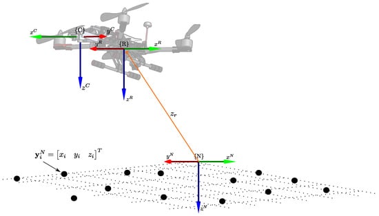
Figure 1.
Parameterization of the 6DOF system.
2.1.2. Visual Observations
To estimate the UAV’s state vector as defined in Equation (1), we assume that the UAV is equipped with a conventional monocular camera. At each time step, the camera captures a set of visual observations corresponding to n stationary 3D landmarks in the environment. The visual measurement for the i-th landmark follows the model:
where denotes the ideal projection of the 3D point onto the image plane, and represents the measurement noise affecting the observation.
The spatial coordinates of the i-th landmark in the navigation frame are expressed as the vector (refer to Figure 1):
The transformation function maps a 3D point in the navigation frame to its 2D coordinates in the image plane, given by
where
The function accounts for the camera’s distortion effects, parameterized by , with representing the undistorted coordinates. The camera’s intrinsic parameters, including the focal length f and the principal point , are considered known through prior calibration. This formulation follows the distortion model proposed in [17].
In Equation (5), the rotation matrix transforms coordinates from the navigation frame to the camera frame . The matrix converts the navigation frame coordinates to the UAV frame based on the orientation parameters in . Meanwhile, defines the transformation from the UAV frame to the camera frame , which is assumed to be predetermined.
The camera’s position in the navigation frame is given by , where
Here, represents the camera’s location relative to the UAV frame and is assumed to be known.
2.1.3. Attitude Measurements
The attitude measurements, denoted as , are expressed as
where the vector represents the actual orientation of the UAV, and accounts for the measurement noise or uncertainty inherent in the orientation readings. These values are obtained directly from the UAV’s Attitude and Heading Reference System (AHRS). In this context, the corresponding measurement model is formulated as
2.1.4. Altitude Measurements
It is assumed that altitude data, referenced in the navigation frame , is provided by an altitude sensor, typically a barometric pressure sensor.
Altitude measurements, denoted as , are defined as
where represents the true altitude of the UAV in the navigation frame , and accounts for the measurement noise or uncertainty inherent to the altitude readings.
The corresponding measurement model is given by
2.1.5. Range-to-Base Measurements
As will be outlined in Section 3, range measurements from the home position (base) to the UAV can significantly improve the observability of the SLAM system. Unlike other aiding measurements, which are typically derived from onboard sensors commonly found in most UAV platforms, range-to-base measurements may necessitate the development of a specialized solution.
Radio Frequency (RF) ranging techniques can be employed to obtain range-to-base measurements. These techniques leverage RF signal properties, such as signal propagation time (Time of Flight, ToF), signal phase (Phase-Based Ranging), or signal strength (Received Signal Strength Indicator, RSSI). Relevant applications of these technologies can be found in [18,19]. Also, Ultra-Wideband (UWB) technology has emerged as a highly practical solution for precise RF-based ranging in UAV applications. UWB systems offer centimeter-level ranging accuracy while maintaining low transmit power and minimal interference with conventional wireless systems. Many commercial UWB modules, such as the Decawave DWM1000, are compact, battery-powered, and easily integrated with small UAV platforms [20].
Range-to-base measurements, denoted as , are defined as
where represents the true range from the base to the UAV in the navigation frame , and accounts for the measurement noise or uncertainty associated with these readings.
The measurement model is given by
It is also important to emphasize that the proposed framework is technology-agnostic regarding the mechanism used to obtain range-to-base data. While UWB offers a practical and efficient implementation option, our theoretical results apply to any system providing sufficiently accurate and bounded range measurements. This flexibility allows adaption to different technologies or operational environments.
2.2. EKF-SLAM
In this work, the local SLAM process is implemented using an Extended Kalman Filter (EKF), though other stochastic filtering methods could also be utilized. The framework follows the traditional EKF-SLAM approach, which involves an iterative cycle of prediction and update steps, as described in [21,22]. Figure 2 depicts the architecture of the proposed EKF-SLAM system.
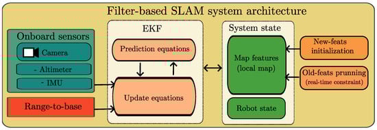
Figure 2.
System architecture.
For EKF-SLAM implementation, the UAV state vector , as defined in Equation (1), is extended by including the states of n map features, , where . These features correspond to the visual landmarks observed by the camera as the UAV explores previously unknown regions of its environment.
The augmented system state, , is expressed as
In the SLAM literature, this extension of the system state is often referred to as feature initialization, which is further detailed in Section 2.2.3.
Thus, using the set of measurements outlined in Section 2.1, the main goal of the proposed monocular-based SLAM method is to estimate the augmented state vector .
2.2.1. Prediction Step
The state vector estimate, , and its covariance matrix, , are propagated over time using the EKF prediction equations:
Here, represents the UAV’s dynamic or kinematic model, is the input vector, is the Jacobian of with respect to the state, and is the Jacobian of with respect to the input. The noise vector models the process noise affecting the state.
In the EKF equations, the notations , , and represent a priori values, a posteriori values, and the “last available value,” respectively. In practice, the propagation described by Equation (13) can be implemented using basic Euler integration.
The discretized kinematic model of the UAV is represented by and is defined as follows:
For this unconstrained constant acceleration model, the process noise covariance matrix is given by , where and . These represent unknown angular and linear velocity impulses modeled as zero-mean Gaussian processes with known covariances and .
The parameters and are correlation time factors that model the rate at which angular and linear velocities decay to zero in the absence of sensor measurements.
Additionally, the matrix defines the relationship between the angular positions and the angular rates :
2.2.2. Update Step
Whenever a measurement becomes available at step k from a sensor , with a measurement model , the state estimate and its covariance matrix are updated using the EKF update equations:
Here, is the Kalman gain, and represents the Jacobian of the measurement model with respect to the state . Additionally, is the measurement noise covariance matrix associated with sensor .
Table 1 provides a summary of the measurements and their corresponding measurement models used to update the estimated system state and its covariance matrix , as described by the update equations in (16). A complete description of these measurements and models can be found in Section 2.1.

Table 1.
Summary of measurements and corresponding models used in the update equations.
2.2.3. Features Initialization
To initialize new map features into the system state , an initialization function must be defined. Here, represents the ith visual measurement used by to compute the pose of .
Once is computed, the system state and covariance matrix are updated as follows:
where is the Jacobian matrix, and represents the measurement noise covariance associated with the measurements .
The undelayed initialization technique described in [23] is used to compute new features . This technique leverages monocular visual measurements and range measurements obtained from an ultrasonic sensor.
2.2.4. Map Management
To ensure a stable computational cost, the system removes outdated or low-quality visual features from its state. A feature is considered “weak” if it exhibits a high ratio of failed matches relative to the number of times it was expected to be detected by the camera. Similarly, a feature is deemed “old” if it has been absent from camera observations for a significant number of instances.
3. Observability Analysis
In this section, the nonlinear observability properties of the proposed system are analyzed. Observability is an intrinsic property of dynamic systems and plays a key role in ensuring the accuracy and stability of state estimation. Furthermore, it has significant implications for the convergence behavior of EKF-based SLAM algorithms.
In particular, we demonstrate that incorporating range-to-base measurements enhances the observability properties of the proposed SLAM system. To offer a more intuitive perspective, consider a UAV flying through a environment while relying only on a monocular camera. Although visual data allows it to estimate motion, the lack of absolute depth results in scale ambiguity, making it difficult to determine how far it has truly moved or how far it is from observed features. Introducing a single range-to-base measurement is like connecting the UAV to a fixed ground station with an invisible rope of known length. This constraint reduces the set of possible positions the UAV can occupy, helping to resolve the scale ambiguity and significantly improving the system’s overall observability. This intuitive example highlights how range information can improve estimation. We now proceed with a formal nonlinear observability analysis of the system.
A system is said to be observable if the initial state at some initial time can be determined from the state transition model , the observation model , and the sequence of measurements collected over a finite time interval . Given the observability matrix , a nonlinear system is said to be locally weakly observable if the condition holds [24].
For the purpose of observability analysis, the state vector of the proposed system is defined as
3.1. Observability Matrix
An observability matrix can be constructed as follows:
Here, denotes the s-th-order Lie derivative [25] of the scalar function with respect to the vector field .
In this work, the rank of the observability matrix in Equation (20) was computed numerically using MATLAB R2023b. The appropriate number of Lie derivative terms was determined iteratively by augmenting with increasingly higher-order derivatives until its rank stabilized.
To facilitate interpretation of the structure in Equation (20), the Lie derivatives corresponding to each type of measurement are color-coded as follows: blue for monocular landmark measurements, red for attitude measurements, orange for altitude measurements, and violet for range measurements (range-to-base station).
A detailed description of the Lie derivatives used to construct Equation (20) is provided in Appendix A.
3.2. Theoretical Results
Two different system configurations were analyzed to evaluate how the observability of the SLAM system is affected by the availability of range measurements: one with range-to-base measurements and one without.
3.2.1. Without Range-to-Base Measurements
In this configuration, the following types of sensor data are available: monocular measurements of the projection of landmarks onto the camera image plane, attitude measurements, and altitude measurements. Based on these measurements, the observability matrix has the following structure:
In this case, to compute (21), zero-order and first-order Lie derivatives are used for each measurement. Consequently, the maximum rank of the observability matrix is given by , where denotes the number of landmarks being measured, and 12 represents the number of UAV states (position, orientation, and their respective velocities). Therefore, is rank-deficient, i.e., . The unobservable modes are spanned by the right nullspace basis of the observability matrix :
where
It is straightforward to verify that lies in the right nullspace of , that is, . From (22), it is evident that the unobservable modes correspond to the x- and y-positions of both the UAV and the landmarks; hence, these states are unobservable. It is important to note that including higher-order Lie derivatives of the measurements in the observability matrix does not improve this result.
3.2.2. With Range Measurements
In this case, the available measurements include monocular observations of the projections of the landmarks onto the camera image plane, attitude measurements, altitude measurements, and range measurements of the UAV relative to a base station (range-to-base). Therefore, the observability matrix has the following structure:
For (24), zero-order and first-order Lie derivatives of the range measurements are incorporated into the observability matrix . As a result, the maximum rank of the observability matrix is . Given that the state dimension is , the system is locally weakly observable, since .
3.3. Remarks on the Theoretical Results
The outcomes of the observability analysis are summarized in Table 2. This table compiles the results discussed above (specifically, Case 4 and Case 5), along with combinations reflecting the availability of different measurement types within the system. It provides a comprehensive overview of the contribution of each measurement type to the overall system observability.
Table 2.
Results of the nonlinear observability analysis of the proposed system. A check mark indicates that the corresponding measurement type is included in the system configuration, whereas a cross mark indicates that it is not.
4. Experimental Results
4.1. Experiments with Virtual Environment
To validate the proposed approach, a C++ implementation was developed using the ROS 2 (Robot Operating System 2) framework [26]. Virtual environments for the experiments were created using Webots, a widely adopted simulator in research, education, and industry. It is commonly used for prototyping and validating robotic algorithms in simulation before deploying them in real-world scenarios [27]. The source code for the visual-based SLAM system implementation is available at [28].
Figure 3 illustrates the two environments used in the virtual experiments. On the left is an open-world, Mars-like environment; on the right is a factory-like indoor environment. In the latter case, the flight trajectory used in the experiments is highlighted to enhance the clarity of the results. The flying robot used in our virtual experiments is a DJI Mavic 2 Pro, which captures image frames using its front-facing monocular camera at a resolution of 400 × 240 pixels and a rate of 30 frames per second. Additionally, we incorporate measurements from the robot’s IMU and altimeter. Since Webots does not natively provide range-to-base measurements, these measurements were emulated by computing the Euclidean distance from the base to the robot’s position and adding Gaussian noise with cm.
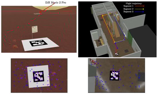
Figure 3.
Virtual environments used in the experiments: an outdoor, open Mars-like environment (left), and an indoor, enclosed factory-like environment (right). The lower plots show a sample camera frame from each environment, captured near the home position.
For each experiment, the drone was commanded to fly over one of the following three predefined trajectories:
- (a)
- Three loops over a simple, rectangle-like trajectory in the Mars-like environment, with a total length of 180 m.
- (b)
- Three loops over a square wave-like trajectory in the Mars-like environment, with a total length of 388 m.
- (c)
- Two loops over a trajectory that explores different areas in the factory-like indoor environment, with a total length of 115 m.
The general methodology used in the experiments was to evaluate the effect of adding range-to-base measurements to the estimated flight trajectory by comparing it with the trajectory obtained in the absence of such measurements.
Figure 4 shows sample results for each of the three flight trajectories, both when range-to-base measurements are excluded and when they are included in the system. As mentioned in Section 2.2.4, to maintain stable computation time, old and weak visual landmarks are removed from the system state. Otherwise, the computational cost per frame would continuously increase, eventually making real-time operation unfeasible. However, removing old landmarks prevents the correction of accumulated estimation drift when the robot revisits previously mapped areas, i.e., loop closure. This effect is clearly visible in the three left-hand plots, where the position estimation error accumulates over time in the absence of range-to-base measurements. In contrast, the three right-hand plots show significant improvements in estimation accuracy when range-to-base measurements are incorporated into the system.
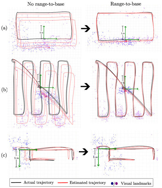
Figure 4.
Comparison between actual and estimated trajectories (top-down XY views), computed with and without range-to-base measurements for flight trajectories (a–c).
To better highlight the effect of including range-to-base measurements in bounding the error drift in position estimation, the Mean Absolute Error (MAE) over time for the estimated position of the robot in the x–y plane was computed over 10 Monte Carlo runs for each flight trajectory, both with and without range-to-base measurements. Figure 5 shows these results. In this case, it is even more evident how the MAE in the estimated x–y position of the robot increases over time without range-to-base measurements, while their inclusion effectively bounds the error.
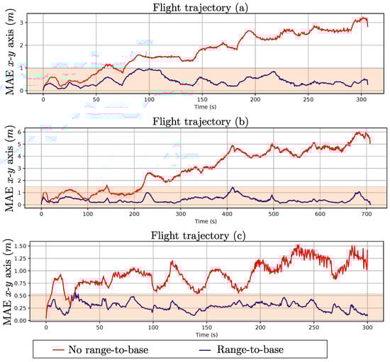
Figure 5.
Comparison of the evolution of Mean Absolute Error (MAE) over time for flight trajectories (a–c) computed with and without range-to-base measurements. Observe that the MAE remain bounded when range-to-base measurements are used.
Table 3 shows the total Monte Carlo MAE over 10 runs for each axis (x, y, z) in each case. It is worth noting that the MAE for the z-axis (altitude) is similar across all cases, as altitude measurements from the robot’s altimeter are fused into the system. On the other hand, as expected from previous results, the total MAE is consistently lower when range-to-base measurements are incorporated into the SLAM system.
Table 3.
Total Monte Carlo Mean Absolute Error (MAE) over 10 runs, computed for the x, y, and z axes for flight trajectories (a), (b), and (c).
4.2. Experiments with Real Data
To further validate our findings, we conducted experiments using real-world data collected in a previous research project. A custom-built quadrotor platform equipped with low-cost onboard sensors was used to gather flight data. The sensor suite consisted of (i) a DX201 DPS camera with a wide-angle lens, (ii) an XL-MaxSonar-EZ0 ultrasonic rangefinder, and (iii) a barometric pressure sensor integrated into the Ardupilot flight controller. Both the camera and ultrasonic sensor were mounted on a budget-friendly TURNIGY two-axis brushless gimbal for stabilization. Data collection was carried out under manual remote control. A ground station received a live video feed via a 5.8 GHz analog link, while telemetry data (including sensor readings and system state) were transmitted over a 915 MHz radio channel. All sensor data, including images, were timestamped and logged for subsequent synchronization. The grayscale camera stream had a resolution of 320 × 240 pixels at 26 frames per second. Barometric pressure readings were sampled at 7 Hz, and ultrasonic range measurements were acquired at 5 Hz. In addition, GPS measurements were recorded at 5 Hz to serve as a reference for the vehicle’s approximate trajectory.
Since no direct range-to-base measurements were available in the dataset, we emulated them by computing the Euclidean distance from each GPS position to the initial GPS fix, expressed in the local coordinate frame. This approach is justified as a reasonable and conservative approximation under the assumption that fixed biases (for example, ephemeris and atmospheric delays) remain constant over the duration of the flight. Once those are removed by referencing the initial GPS point, the dominant error source is measurement noise, which for standard civilian GPS under good satellite visibility is typically around 1 m RMS in horizontal position. In contrast, a low-cost UWB module such as the Decawave DWM1000 (which could be used in a practical implementation for range-to-base measurements) can achieve sub-meter ranging accuracy, typically around 0.2 to 0.3 m, assuming proper calibration of antenna delays and signal strength compensation.
Figure 6 shows an aerial view of the outdoor environment where the dataset was collected, along with one of the estimated flight trajectories overlaid on the GPS measurements (left plot). The custom-built quadrotor platform used for data collection is shown in the upper-right plot, and an example frame from the onboard camera, which highlights the visual landmarks being tracked at that moment, is shown in the lower-left plot. For these experiments, a MATLAB implementation of the proposed approach was used. This version was specifically tailored to operate with the recorded dataset.
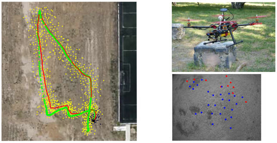
Figure 6.
Overview of the real-world experiment. (Left): aerial view of the outdoor environment with overlaid GPS measurements and estimated flight trajectory. (Upper right): custom-built quadrotor platform used for data collection. (Lower right): sample onboard camera frame showing tracked visual landmarks.
It is important to recall that the main contribution of this work is to demonstrate that integrating range-to-base measurements into a filter-based monocular SLAM system can substantially improve its observability properties. This, in turn, has the significant benefit of bounding the estimation error. In other words, the theoretical findings regarding observability are general in nature and not specific to a particular system implementation. To support this claim, in addition to the method presented in Section 2, the well-known inverse depth (ID) parameterization for monocular SLAM introduced in [29] was also tested. The same MATLAB implementation was extended to run this alternative method on the same dataset in order to validate the benefits of incorporating range-to-base measurements into different filter-based monocular SLAM approaches.
Figure 7 shows the results obtained after running both methods: (i) the method proposed in this work (upper plots) and (ii) the ID-based monocular SLAM method (lower plots), using the previously described dataset. For each method, the results are shown without range-to-base measurements (left plots) and with range-to-base measurements integrated (right plots).
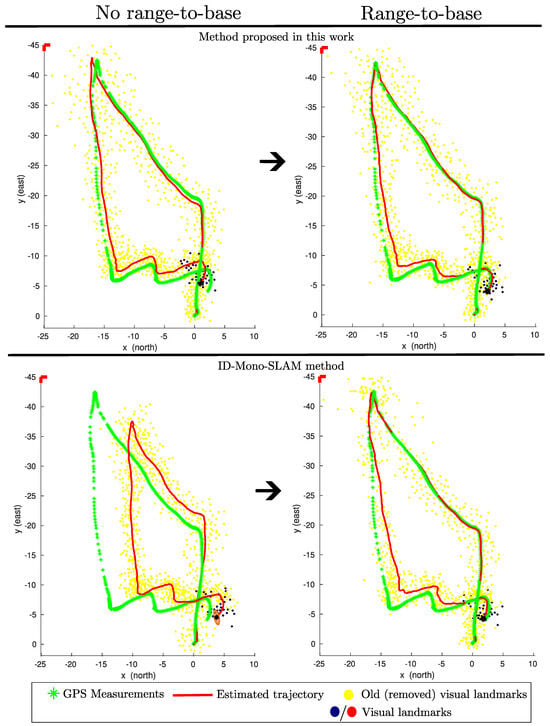
Figure 7.
Estimated UAV trajectories using the proposed method (top) and ID-based monocular SLAM (bottom), both without (left) and with (right) range-to-base measurements. GPS data is shown as a reference. Integration of range-to-base data significantly improves accuracy and bounds estimation error in both approaches.
In all cases, the GPS measurements serve as a close reference to the actual flight trajectory. For the proposed method without range-to-base measurements, the estimated trajectory appears reasonable. However, as expected, it exhibits some drift due to the removal of old visual landmarks in order to maintain real-time operation. When range-to-base measurements are included, the estimation error becomes bounded, which aligns with the results observed in the virtual experiments. Notably, the error is significantly reduced near the end of the flight when the UAV returns close to its home position.
For the ID-based monocular SLAM method without range-to-base measurements, the estimated trajectory deviates considerably from the actual trajectory. One key difference between this method and the one proposed in this work is that the latter also incorporates measurements from an onboard sonar, which helps improve the initialization of visual features in the state estimator. This difference may explain the performance gap when no range-to-base measurements are used. When range-to-base measurements are added to the ID-based monocular SLAM method, the estimated trajectory improves substantially. In this case, it is particularly noticeable that the estimation error is also bounded and minimized toward the end of the trajectory.
5. Discussion
The nonlinear observability analysis shows that when range-to-base measurements are included in the SLAM system, the system state becomes observable. This is a significant theoretical result because nonlinear observability is a necessary condition for keeping the estimation error bounded. Moreover, the results from the virtual experiments demonstrate that including range-to-base measurements enables the estimation error in the proposed EKF-based SLAM system to remain effectively bounded, even when old map features are removed from the system state. These results are promising as they suggest that for various aerial robotics applications, adding range-to-base measurements to a standard monocular SLAM system may be sufficient to address the state estimation problem in GPS-denied environments.
To support the theoretical and simulated findings, additional experiments were conducted using a real-world dataset collected with a custom quadrotor platform. These experiments confirmed the earlier conclusions: integrating range-to-base measurements significantly reduced estimation drift and helped bound the error in both the proposed method and an alternative monocular SLAM approach. Without these measurements, both systems exhibited degraded performance, particularly when visual features were lost or removed. These outcomes reinforce the generality of the theoretical analysis as similar improvements were observed even when applied to a different SLAM formulation.
It is important to note, however, that the real-data experiments involved certain approximations. Specifically, direct range-to-base measurements were not available in the dataset and were emulated by computing the Euclidean distance from each GPS position to the initial GPS fix. This approximation is considered reasonable and conservative. Nevertheless, it does not fully replicate the behavior or accuracy of dedicated range sensors such as UWB modules. Consequently, while the validation with real data supports the main claims of this work, further testing with actual range-to-base sensors would provide stronger practical evidence.
Overall, these experimental results reinforce the practical relevance of the proposed approach and suggest that the inclusion of range-to-base data, despite requiring additional hardware, can yield substantial performance benefits in realistic scenarios.
While the integration of range-to-base measurements into SLAM systems presents significant advantages, it is worth emphasizing that, unlike widely adopted aiding sensors such as AHRS units and altimeters (which are typically standard on most UAV platforms), range-to-base sensing often depends on custom hardware and emerging technologies that are not yet well established in UAV navigation. As a result, although the findings presented here are encouraging, further investigation is needed to fully assess the feasibility and robustness of this approach across a broad range of real-world conditions.
6. Conclusions
In this work, we introduced a novel EKF-based SLAM system that leverages monocular vision and is specifically designed for UAV navigation in GPS-denied environments. The core contribution lies in demonstrating that the incorporation of range-to-base measurements enables the estimation error to remain bounded, even when older visual landmarks are systematically removed from the system state to maintain consistent computational performance.
While numerous existing approaches address the challenge of UAV navigation without GPS support (e.g., Refs. [30,31,32]), many of them rely on loop-closure strategies to reduce accumulated drift or focus primarily on slowing the error growth. In contrast, the method proposed here is designed to keep the estimation error bounded throughout the entire flight trajectory, offering a more robust alternative for long-duration autonomous missions.
Beyond the specific implementation presented, the theoretical findings of this work are of general relevance. In particular, the improved observability achieved through the addition of range-to-base measurements is applicable to a broader class of filter-based monocular SLAM systems. This makes the proposed approach a valuable contribution for enhancing state estimation reliability in GPS-denied aerial navigation across various platforms and configurations.
Author Contributions
The contributions of each author are as follows: Conceptualization, R.M. and J.-C.T.; methodology, R.M. and J.-C.T.; software, R.M. and J.-C.T.; validation, J.-C.T. and A.G.; investigation, R.M. and J.-C.T.; resources, A.G.; writing—original draft preparation, R.M. and J.-C.T.; writing—review and editing, A.G.; visualization, J.-C.T. and A.G.; supervision, R.M. and A.G.; funding acquisition, A.G. All authors have read and agreed to the published version of the manuscript.
Funding
This research received no external funding.
Data Availability Statement
The source code will be available in [28] after acceptance.
Acknowledgments
During the preparation of this manuscript, the author(s) used ChatGPT-4 for language and grammar checking. The author(s) have reviewed and edited the output and take full responsibility for the content of this publication.
Conflicts of Interest
The authors declare no conflicts of interest. The funders had no role in the design of the study; in the collection, analyses, or interpretation of data; in the writing of the manuscript; or in the decision to publish the results.
Abbreviations
The following abbreviations are used in this manuscript:
| SLAM | Simultaneous Localization and Mapping |
| UAV | Unmanned Aerial Vehicle |
| GPS | Global Positioning System |
| IMU | Inertial Measurement Unit |
| AHRS | Attitude and Heading Reference System |
| MAE | Mean Absolute Error |
| NED | North–East–Down |
| RF | Radio Frequency |
| ToF | Phase-Based Ranging |
| RSSI | Received Signal Strength Indicator |
| EKF | Extended Kalman Filter |
| ROS | Robotics Operating System |
Appendix A. Lie Derivatives of Measurements
In this appendix, the Lie derivatives corresponding to each measurement equation used in Section 3 are presented.
From Equation (4), the zero-order Lie derivative of the landmark projection model is given by
where
with
and
Note that denotes the antisymmetric matrix of the vector (.). The first-order Lie derivative for landmark projection model is
where
with
and
From Equation (7), the zero-order Lie derivative can be obtained for the attitude measurement model:
The first-order Lie derivative for the attitude measurement model is
From Equation (9), the zero-order Lie derivative can be obtained for the altitude measurement model:
with
The first-order Lie derivative for the altitude measurement model is
From Equation (11), the zero-order Lie derivative can be obtained for the range measurement model:
The first-order Lie derivative for the range measurement model is
where
References
- Mur-Artal, R.; Tardos, J.D. ORB-SLAM2: An Open-Source SLAM System for Monocular, Stereo, and RGB-D Cameras. IEEE Trans. Robot. 2017, 33, 1255–1262. [Google Scholar] [CrossRef]
- Campos, C.; Elvira, R.; Rodríguez, J.J.G.; M. Montiel, J.M.; D. Tardós, J. ORB-SLAM3: An Accurate Open-Source Library for Visual, Visual–Inertial, and Multimap SLAM. IEEE Trans. Robot. 2021, 37, 1874–1890. [Google Scholar] [CrossRef]
- Qin, T.; Li, P.; Shen, S. VINS-Mono: A Robust and Versatile Monocular Visual-Inertial State Estimator. IEEE Trans. Robot. 2018, 34, 1004–1020. [Google Scholar] [CrossRef]
- Huang, G. Visual–Inertial Navigation: A Concise Review. In Proceedings of the IEEE International Conference on Robotics and Automation (ICRA), Montreal, QC, Canada, 20–24 May 2019; pp. 9572–9582. [Google Scholar] [CrossRef]
- Rosen, D.M.; Doherty, K.J.; Espinoza, A.T.; Leonard, J.J. Advances in Inference and Representation for Simultaneous Localization and Mapping. Annu. Rev. Control. Robot. Auton. Syst. 2021, 4, 215–242. [Google Scholar] [CrossRef]
- Ding, Y.; Xiong, Z.; Xiong, J.; Cui, Y.; Cao, Z. OGI-SLAM2: A Hybrid Map SLAM Framework Grounded in Inertial-Based SLAM. IEEE Trans. Instrum. Meas. 2022, 71, 1–14. [Google Scholar] [CrossRef]
- Lee, W.; Yang, Y.; Huang, G. Efficient Multi-sensor Aided Inertial Navigation with Online Calibration. In Proceedings of the 2021 IEEE International Conference on Robotics and Automation (ICRA), Xi’an, China, 30 May–5 June 2021; pp. 5706–5712. [Google Scholar] [CrossRef]
- Zhao, M.; Zhou, D.; Song, X.; Chen, X.; Zhang, L. DiT-SLAM: Real-Time Dense Visual-Inertial SLAM with Implicit Depth Representation and Tightly-Coupled Graph Optimization. Sensors 2022, 22, 3389. [Google Scholar] [CrossRef] [PubMed]
- Lee, K.W.; Wijesoma, W.S.; Guzman, J.I. On the Observability and Observability Analysis of SLAM. In Proceedings of the 2006 IEEE/RSJ International Conference on Intelligent Robots and Systems, Beijing, China, 9–13 October 2006; pp. 3569–3574. [Google Scholar] [CrossRef]
- Forster, C.; Carlone, L.; Dellaert, F.; Scaramuzza, D. On-Manifold Preintegration for Real-Time Visual–Inertial Odometry. IEEE Trans. Robot. 2017, 33, 1–21. [Google Scholar] [CrossRef]
- Li, X.; Zhang, Y.; Wang, J. IVU-AutoNav: Integrated Visual and UWB Framework for Autonomous Navigation. Drones 2025, 9, 162. [Google Scholar] [CrossRef]
- Nguyen, T.H.; Yuan, S.; Xie, L. VR-SLAM: A Visual-Range Simultaneous Localization and Mapping System using Monocular Camera and Ultra-wideband Sensors. arXiv 2023, arXiv:2303.10903. [Google Scholar]
- Hong, M.; Chen, Y.; Wu, Z. UVIO: Adaptive Kalman Filtering UWB-Aided Visual-Inertial SLAM System for Complex Indoor Environments. Remote Sens. 2024, 16, 3245. [Google Scholar] [CrossRef]
- Radwan, A.; Tourani, A.; Bavle, H.; Voos, H.; Sanchez-Lopez, J.L. UAV-Assisted Visual SLAM Generating Reconstructed 3D Scene Graphs in GPS-Denied Environments. In Proceedings of the 2024 International Conference on Unmanned Aircraft Systems (ICUAS), Crete, Greece, 4–7 June 2024; pp. 1109–1116. [Google Scholar] [CrossRef]
- Karrer, M.; Schmuck, P.; Chli, M. CVI-SLAM—Collaborative Visual-Inertial SLAM. IEEE Robot. Autom. Lett. 2018, 3, 2762–2769. [Google Scholar] [CrossRef]
- Scaramuzza, D.; Zhang, Z. Visual-Inertial Odometry of Aerial Robots. arXiv 2019. [Google Scholar] [CrossRef]
- Bouguet, J. Camera Calibration Toolbox for Matlab. 2008. Available online: https://data.caltech.edu/records/jx9cx-fdh55 (accessed on 10 August 2025).
- Wu, D.; Bao, L.; Li, R. UWB-Based Localization in Wireless Sensor Networks. Int. J. Commun. Netw. Syst. Sci. 2009, 2, 407–421. [Google Scholar] [CrossRef]
- Xu, H.; Zhang, W.; Yang, L. Wireless Localization and Ranging with Ultra-Wideband Signals. In Proceedings of the 2011 IEEE International Conference on Ultra-Wideband (ICUWB), Bologna, Italy, 14–16 September 2011; pp. 580–584. [Google Scholar] [CrossRef]
- Peña Queralta, J.; Martínez Almansa, C.; Schiano, F.; Floreano, D.; Westerlund, T. UWB-based system for UAV Localization in GNSS-Denied Environments: Characterization and Dataset. In Proceedings of the IEEE/RSJ International Conference on Intelligent Robots and Systems (IROS), Las Vegas, NV, USA, 25–29 October 2020. [Google Scholar] [CrossRef]
- Durrant-Whyte, H.; Bailey, T. Simultaneous localization and mapping: Part I. IEEE Robot. Autom. Mag. 2006, 13, 99–110. [Google Scholar] [CrossRef]
- Bailey, T.; Durrant-Whyte, H. Simultaneous localization and mapping (SLAM): Part II. IEEE Robot. Autom. Mag. 2006, 13, 108–117. [Google Scholar] [CrossRef]
- Urzua, S.; Munguía, R.; Grau, A. Vision-based SLAM system for MAVs in GPS-denied environments. Int. J. Micro Air Veh. 2017, 9, 283–296. [Google Scholar] [CrossRef]
- Hermann, R.; Krener, A. Nonlinear controllability and observability. IEEE Trans. Autom. Control 1977, 22, 728–740. [Google Scholar] [CrossRef]
- Slotine, J.J.E.; Li, W. Applied Nonlinear Control; Prentice Hall: Englewood Cliffs, NJ, USA, 1991. [Google Scholar]
- Macenski, S.; Foote, T.; Gerkey, B.; Lalancette, C.; Woodall, W. Robot Operating System 2: Design, architecture, and uses in the wild. Sci. Robot. 2022, 7, eabm6074. [Google Scholar] [CrossRef] [PubMed]
- Cyberbotics Ltd. Webots: Professional Mobile Robot Simulation Software. 2023. Available online: https://www.cyberbotics.com/ (accessed on 10 June 2025).
- Source Code. Available online: https://github.com/rodrigo-munguia/EKF-MonoSLAM-Range-To-Base (accessed on 10 August 2025).
- Civera, J.; Davison, A.J.; Montiel, J.M.M. Inverse Depth Parametrization for Monocular SLAM. IEEE Trans. Robot. 2008, 24, 932–945. [Google Scholar] [CrossRef]
- Bry, A.; Bachrach, A.; Roy, N. State estimation for aggressive flight in GPS-denied environments using onboard sensing. In Proceedings of the 2012 IEEE International Conference on Robotics and Automation, St Paul, MN, USA, 14–18 May 2012; pp. 1–8. [Google Scholar] [CrossRef]
- Singh, A.K.; Duba, P.K.; Rajalakshmi, P. Deep RL-based Autonomous Navigation of Micro Aerial Vehicles in a Complex GPS-Denied Indoor Environment. arXiv 2025, arXiv:2504.05918. [Google Scholar]
- Balamurugan, G.; Valarmathi, J.; Naidu, V.P.S. Survey on UAV navigation in GPS denied environments. In Proceedings of the 2016 International Conference on Signal Processing, Communication, Power and Embedded System (SCOPES), Paralakhemundi, India, 3–5 October 2016; pp. 198–204. [Google Scholar] [CrossRef]
Disclaimer/Publisher’s Note: The statements, opinions and data contained in all publications are solely those of the individual author(s) and contributor(s) and not of MDPI and/or the editor(s). MDPI and/or the editor(s) disclaim responsibility for any injury to people or property resulting from any ideas, methods, instructions or products referred to in the content. |
© 2025 by the authors. Licensee MDPI, Basel, Switzerland. This article is an open access article distributed under the terms and conditions of the Creative Commons Attribution (CC BY) license (https://creativecommons.org/licenses/by/4.0/).