Abstract
The tandem tilt-wing UAV features an advanced aerodynamic layout design and is regarded as a solution for small-scale urban air mobility. However, the tandem wing configuration exhibits complex aerodynamic interactions between the front and rear wings during cruise flight and the wing tilt transition process. The objective of this paper is to investigate the aerodynamic coupling characteristics between the front and rear wings of the tandem tilt-wing UAV under level flight and tilt transition conditions while also assessing the influence of the propellers on the aircraft’s aerodynamic performance. Through CFD numerical analysis, the aerodynamic characteristics of various aircraft components are examined at different angles of attack and wing tilt angles, and the underlying reasons for the observed differences and variations are explored. The results indicate that, during level flight, the aerodynamic interference between the wings is primarily dominated by the detrimental influence of the front wing on the rear wing. During the tilt transition process, mutual interactions between the front and rear wings occur as wing tilt angle changes, leading to more drastic variations in lift coefficients and increased control difficulty. However, the propeller’s effect contributes to smoother changes in lift and drag, thereby enhancing aircraft stability.
1. Introduction
Vertical takeoff and landing (VTOL) fixed-wing UAVs (Unmanned Aerial Vehicles) combine the advantages of fixed-wing aircraft, such as high speed, long range, and extended endurance, with the vertical takeoff and landing capabilities of helicopters [1]. Among VTOL fixed-wing aircraft, tiltrotor configurations remain predominant, exemplified by the U.S. V-22 Osprey [2], with hundreds currently in service. In recent years, with the growing demand for urban small-scale aviation, Electric Vertical Takeoff and Landing (eVTOL) UAVs have gained increasing attention. Concurrently, rapid advancements in battery technology, electric propulsion for drones, distributed propulsion design, new composite materials, manufacturing processes, numerical simulation methods, and flight control technologies have provided substantial technical support for the development of tilt-wing UAV [3,4,5]. The tandem tilt-wing UAV is a novel configuration of VTOL fixed-wing aircraft, featuring two parallel sets of front and rear wings. Compared to conventional layouts, this design improves the lift-to-drag ratio while reducing structural strength requirements [6,7], offering significant advantages for urban air mobility.
Compared to tiltrotor UAV, a tilt-wing UAV exhibits superior lift characteristics during the transition phase. Unlike tiltrotor UAVs, where propellers are mounted at the wingtips, in tilt-wing UAVs, the propellers are rigidly coupled to and tilt together with the wings, maintaining their relative positions. During vertical takeoff and landing, the wing plane remains perpendicular to the propeller plane, minimizing the wing’s obstruction of the propeller. This ensures that the wing surface remains aligned with the airflow without hindering the downwash generated by the propeller, resulting in higher propeller efficiency in rotor mode. Additionally, during the transition phase, the downwash from the propeller can be utilized to generate continuous lift on the wings, thus enhancing the stability of the flight mode transition [8].
Currently, researchers worldwide have conducted extensive studies on the aerodynamic characteristics of tiltrotor and tilt-wing UAVs during the transition phase, primarily using wind tunnel experiments and numerical simulations.
In the field of wind tunnel experiments, Tom C. A. Stokkermans et al. [9] investigated how the interaction of side-by-side propeller configurations affects thrust, power, forces in plane, and moments out of plane. They employed total pressure and planar particle image velocimetry measurements to study slipstream characteristics. Alex Zanotti et al. [10] examined the aerodynamic interactions between two tandem propellers by varying their lateral separation distance and tilt angle while maintaining a fixed axial distance. They also studied the effects of slowly changing the inflow angle and velocity, focusing on the aerodynamic interactions during typical transition phases of eVTOL flight envelopes. One of the most representative experimental studies on tilt-wing UAVs was conducted by NASA [11], which utilized the Langley 12-foot Low-Speed Wind Tunnel to test the LA-8 quad tilt-wing UAV. The experiment selected 14 test points for wing tilt angles ranging from 56 to 14 degrees, collecting aerodynamic data, including longitudinal force, lateral force, and moment coefficients during different flight phases. In China, Liu Jifu et al. [12] conducted wind tunnel force measurements on a small multi-propeller tilt-wing UAV, examining various states such as different wing tilt angles, control surface angles, and throttle settings during the transition phase. They analyzed the control characteristics and strategies for different wing tilt angles during transition.
In terms of numerical simulations, Wayne Johnson et al. [13,14] combined wind tunnel test data from a standalone rotor-nacelle model of a tiltrotor aircraft with the aerodynamic analysis software CAMRAD to study the aerodynamic performance of tiltrotors in helicopter mode, particularly the impact of wake models on the results. Chunhua Sheng et al. [15] used a Navier–Stokes computational fluid dynamics (CFD) solver to predict and analyze the unsteady flow field and aerodynamic performance of the Bell Boeing Quad Tilt Rotor wind tunnel model. Vinit Gupta et al. [16] employed CFD methods to simulate forward flight scenarios: without propellers, with propellers, and with counter-rotating propellers, to analyze the effects of propeller downwash on a simplified quadrotor aircraft. Atsushi Shinozuka et al. [17] conducted wind tunnel experiments and unsteady Reynolds-averaged Navier–Stokes (URANS) analyses on a half-model of the LA-8 wind tunnel model, validating the effectiveness of URANS in evaluating the aerodynamic characteristics of tandem tilt-wing aircraft during cruise and transition phases. Qingjin Huang et al. [18] used the momentum source method to simulate the effects of propellers on airflow in a tilt-wing model, finding significant differences in forces acting on the tilt-wing aircraft between steady-state calculations at fixed tilt angles and unsteady calculations with continuous tilt angle changes. Li Peng et al. addressed the challenge of generating high-quality integrated structured grids for complex tiltrotor aircraft by introducing a new predefined boundary nesting strategy, combining “reverse boundary” and “Local Direct-Map” (LDP) techniques to establish a predefined boundary nesting grid method [19]. They conducted preliminary numerical simulations of hover, cruise, and transition flight states for tiltrotor aircraft using CFD methods [20]. Later, they integrated a block grid strategy with the nesting grid method, proposing and developing a novel nesting grid generation method suitable for the aerodynamic interference analysis of tiltrotor aircraft [21]. Wang Zonghui et al. [22] conducted computational simulations of unsteady aerodynamic interactions in the tiltrotor UAV flow field using the Delayed Detached Eddy Simulation (DDES) methodology. The analysis revealed that separated vortices generated by the tiltrotor segments collided with the rotor downwash, forming substantial wake interaction zones near the wingtips. This phenomenon subsequently induced downwash effects on the inboard fixed-wing sections, resulting in measurable lift reduction. Wang Yucheng et al. [23] integrated the momentum source method with sliding mesh techniques to simulate the transition phase of a tilt-wing UAV. By implementing momentum sources through functional curve fitting, they achieved smoother altitude-stabilized tilting, thereby ensuring enhanced smoothness in the force distribution curves during the return-to-level transition phase. Yang Pengqian et al. [24] investigated the strongly coupled nonlinear aerodynamic phenomena of tandem-wing configured aircraft under low-speed, high-angle-of-attack conditions. Their numerical simulations elucidated the coupled aerodynamic mechanisms between front and rear wings at high angles of attack, proposing a novel full-motion rear wing control strategy for such flight regimes.
During the transition between horizontal flight and vertical takeoff and landing in a tandem tilt-wing UAV, the wings and propellers simultaneously tilt by 90° around the wing axis. This process induces significant flow field variations and turbulent airflow around the UAV, accompanied by complex aerodynamic interactions among front and rear wings, front and rear propellers, and fuselage. The resultant drastic fluctuations in lift, drag, and propeller thrust adversely affect the stability and transition smoothness of the aircraft. In previous aerodynamic studies of tandem tilt-wing aircraft, researchers predominantly focused on global performance metrics, lacking direct isolation of interference effects between the front and rear wings. This paper presents a novel aerodynamic configuration for a tandem-tiltwing UAV and employs numerical simulations to analyze its aerodynamic characteristics during both cruise flight and transition phases. A numerical methodology incorporating the Multiple Reference Frame (MRF) approach was developed to simulate rotor dynamics, establishing a robust framework for investigating steady-state flow field during wing tilting transitions. This research focuses on analyzing aerodynamic interference characteristics among the propellers, tandem wings, and fuselage during the transition state.
The remainder of this paper is organized as follows: Section 2 delineates the UAV model and numerical methodology, including boundary condition specifications and meshing strategies. Section 3 examines aerodynamic coupling between tandem wings during cruise flight conditions across a broad angle-of-attack range. Section 4 investigates the transitional aerodynamics of the tilt-wing configuration, analyzing steady-state aerodynamic interactions among wing components and the fuselage at varying tilt angles. The effect of the propellers on the aerodynamic performance of the front wing, rear wing, and fuselage is also explored. Conclusions are presented in Section 5.
2. Numerical Simulation Method
2.1. Flow Field Governing Equations and Turbulence Model
The tandem tilt-wing UAV discussed in this paper is primarily designed for low-Reynolds-number conditions. The governing equations for the numerical simulation of the flow field are the Navier–Stokes (NS) equations. For three-dimensional incompressible viscous flow, the specific equations are as follows [25]:
In the above equations, ρ is the density of air; t is time; u, v, and w are the velocity components of the fluid at point (x, y, z) at time t in the three coordinate directions, respectively; p is the dimensionless pressure; fx, fy, and fz are the unit mass forces acting on point (x, y, z) in the three coordinate directions; and μ is the dynamic viscosity of the fluid.
The vector form of the equations is as follows:
Turbulence modeling methodologies can be broadly categorized into Reynolds-Averaged Navier–Stokes (RANS) models, Large Eddy Simulation (LES), and Direct Numerical Simulation (DNS) [26,27,28,29]. The RANS framework resolves time-averaged Navier–Stokes equations through temporal filtering of turbulent fluctuations, offering reduced computational demands while capturing essential turbulent dynamics. This approach encompasses numerous sub-models: Standard k-epsilon model, RNG k-epsilon model, Shear Stress Transport (SST) k-omega model, and Spalart–Allmaras one-equation model. LES employs spatial filtering to explicitly resolve large-scale eddies while modeling subgrid-scale turbulence, incurring higher computational costs than RANS. DNS directly solves transient Navier–Stokes equations without turbulence modeling assumptions, theoretically resolving all turbulent scales. However, its excessive computational requirements currently limit application to laboratory-scale investigations of low-Reynolds-number configurations [30].
This paper employs the SST k-omega turbulence model, which synergistically integrates k-epsilon formulations in free-stream regions with k-omega treatments near wall boundaries. This hybrid approach incorporates turbulent shear stress transport through its revised eddy viscosity definition. As a low-Reynolds-number model, it maintains resolution requirements comparable to baseline k-omega formulations while addressing critical limitations inherent to both k-omega and k-epsilon paradigms, particularly in adverse pressure gradient flows.
2.2. Computational Model and Boundary Condition Setup
The subject of this research is a tandem tilt-wing UAV, with preliminary three-dimensional model schematics presented in Figure 1. Key design parameters are summarized in Table 1. The configuration features two parallel front and rear straight wings incorporating large wingtip endplates that serve dual aerodynamic functions: vertical stabilizer effectiveness and lift enhancement through induced drag reduction [31]. The front and rear wings along with their wingtip endplates were deliberately designed to be identical in size. This configuration enables a direct comparative analysis of the aerodynamic forces acting on the front versus rear wings (including wingtip endplates) and facilitates a clearer investigation of aerodynamic interference between the front and rear wings. Airfoil selection employs the high-lift NACA 4412 profile for main wings and symmetrical NACA 0012 for endplates. To optimize computational fluid dynamics (CFD) analysis fidelity, secondary components with negligible aerodynamic influence (e.g., landing gear) were omitted from the simulation model. The CFD aerodynamic simulation for this project was completed using the solver developed by our project team.
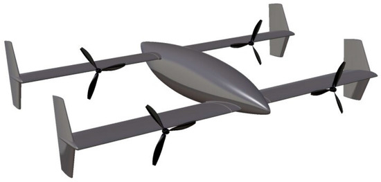
Figure 1.
D model of the tandem tilt-wing UAV.

Table 1.
General parameters of the tandem tilt-wing UAV.
The model exhibits perfect bilateral symmetry, enabling the adoption of a half-model configuration for aerodynamic analysis to optimize computational efficiency. The computational domain is partitioned into different regions: the external flow domain and the propeller-actuated zone. The external flow domain is configured as a rectangular prism measuring 15 m × 6.7 m × 5.75 m, scaled to approximately 10 times the aircraft length in horizontal and vertical dimensions, and 5 times the wingspan laterally.
This study employs the Multiple Reference Frame (MRF) method to simulate rotor rotation by assigning rotational motion attributes to the designated rotor zones. As shown in Figure 2, the computational domain is partitioned with specific boundary conditions: the interface between the rotor disk region and outer flow field is defined as “interface”, symmetry planes in the outer domain are set as “symmetry”, the fuselage surface is treated as “wall”, the downstream boundary is configured as “outlet”, and the remaining three boundaries are designated as “inlet”. The surface meshing scheme for the fuselage and propeller components (Figure 3) utilizes unstructured grids with local refinement near critical aerodynamic regions, particularly around the fuselage and rotor flow field. Multiple layers of refined grids were applied to the aircraft surface.
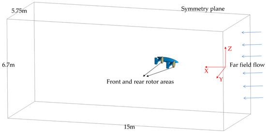
Figure 2.
Computational domain.
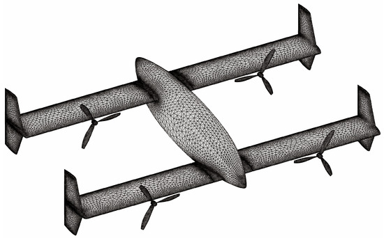
Figure 3.
UAV surface mesh.
Preliminary aerodynamic analysis of the selected propeller established the relationship between propeller efficiency (η) and rotational speed (n) (Figure 4), At 6000 RPM, propeller efficiency remains relatively high, and this rotational speed is adopted for the cruise condition and wing tilt transition. The freestream velocity is maintained at the UAV’s cruise speed of 25 m/s.
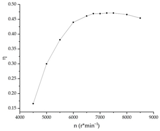
Figure 4.
Propeller efficiency (η) curve as a function of propeller speed (n).
To systematically investigate the tandem tilt-wing configuration’s aerodynamic characteristics, baseline simulations were conducted under cruise flight conditions (25 m/s freestream) with angle of attack(α) variations spanning −6° to 38°. This extended α range enables comprehensive characterization of aerodynamic coupling effects between front and rear wings. For transitional phase analysis, in the physical process, the wings and rotors undergo continuous rotation from 0° to 90°. Under the quasi-steady assumption—where an infinitely slow transition approximates static equilibrium at each tilt angle—10 discrete reference points between 0° and 90° were selected to investigate the aerodynamic interference mechanisms among the front wing, rear wing, and rotor system. Aerodynamic properties are evaluated under fixed conditions (α = 0°, 25 m/s freestream), and, subsequently, a systematic investigation was performed, culminating in a comprehensive assessment of the UAV’s aerodynamic characteristics throughout the entire transition process.
2.3. Grid Independence Verification
Grid quality and density exert significant influence on computational accuracy, necessitating rigorous mesh independence verification. The lift of the front wing at 10° wing tilt angle and 0° angle of attack was selected as the convergence metric. The variation in the front wing lift with the number of grid cells in the flow field model is shown in Figure 5. After balancing computational resources and the accuracy of the results, the final model was determined to have approximately 3.2 million grid cells.
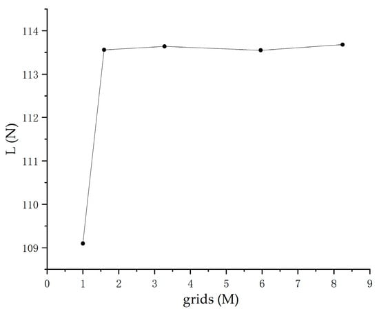
Figure 5.
Front wing lift (N) variation vs. flow field model grid number (million).
3. Aerodynamic Characteristics of Tandem-Wing Configuration in Cruise Flight
3.1. Computational Model Setup
To study the aerodynamic coupling effects between the front and rear wing, three computational models were established: Front-Wing-Fuselage (FW-F) model, Rear-Wing-Fuselage (RW-F) model, and Complete Aircraft (CA) model, as shown in Figure 6. All domain partitioning follows Figure 2 as the standard. Following model configuration setup, flow field simulation and analysis were sequentially performed for each model, with a simplified workflow diagram presented in Figure 7; subsequent data processing and analysis were then conducted.
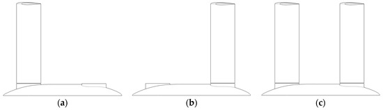
Figure 6.
Computational model: (a) FW-F model; (b) RW-F model; (c) CA model.
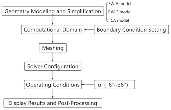
Figure 7.
Flowchart of flow field simulation analysis in cruise flight.
In the CA model, the aerodynamic force coefficients of the front wing, rear wing, and total aircraft were compared, along with their variation patterns with angles of attack. At the same time, the aerodynamic data of the FW-F model were compared with those of the CA model, and the aerodynamic data of the RW-F model were also compared with those of the CA model. This approach was used to investigate the aerodynamic interference of the front wing on the rear wing and the aerodynamic interference of the rear wing on the front wing.
3.2. Aerodynamic Characteristics of Tandem-Wing Configuration
The curves of lift and drag coefficients (CL and CD) for each component of the propeller-off aircraft configuration, as a function of the angle of attack (α), are shown in Figure 8.
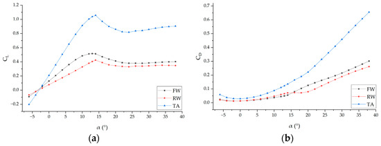
Figure 8.
Lift and drag coefficients (CL and CD) for each component of the propeller-off aircraft during the cruise flight: (a) CL curves; (b) CD curves.
In all aerodynamic coefficient calculations within this study, the reference area “S” in the aerodynamic force formulas consistently employs the total wing reference area (sum of the front and rear wing reference areas), which means that the total aircraft lift coefficient is derived by applying the lift coefficient formula to the combined lift contributions from the front wing, rear wing, and fuselage.
From Figure 8a, it can be observed that the trends of CL for the front wing (FW), rear wing (RW), and the total aircraft (TA) are consistent. However, the CL of the rear wing is significantly lower than that of the front wing. The critical angle of attack for the front wing is 13°, while, for the rear wing and the total aircraft, it is 14°. Before reaching the critical angle of attack, the slope of the front wing’s CL is significantly steeper than that of the rear wing.
From Figure 8b, CD for the front wing, rear wing, and the total aircraft first decreases and then increases. CD for both the front and rear wings reaches their minimum values at −2°, while CD for the total aircraft reaches its minimum at 0°. Between 2° and 14°, the CD of the rear wing is higher than the CD of the front wing; for other angles of attack, the CD of the rear wing is lower than the CD of the front wing. The trends of the CD for the front and rear wings are generally consistent, but they differ at certain specific angles. In the range of 14° to 20°, the CD of the front wing increases significantly, while the CD of the rear wing increases only slightly, causing the CD of the front wing to surpass the CD of the rear wing.
The lift-to-drag ratio (L/D) of the propeller-off aircraft model is shown in Figure 9. As the angle of attack increases, L/D initially increases and then decreases. The front wing reaches its maximum L/D at a 6° angle of attack, while the rear wing and the total aircraft reach their maximum values at a 4° angle of attack. Before a 16° angle of attack, the L/D of the front wing is greater than that of the total aircraft, and the L/D of the total aircraft is greater than the L/D of the rear wing. However, after a 16° angle of attack, this relationship reverses: the L/D of the rear wing becomes greater than that of the total aircraft, and the L/D of the total aircraft becomes greater than that of the front wing. As the angle of attack continues to increase, the L/D of the front wing, rear wing, and the total aircraft eventually converge to similar values.
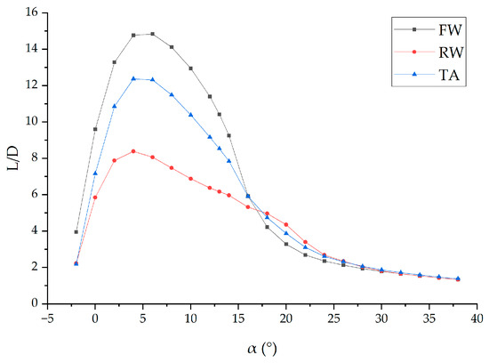
Figure 9.
L/D for each component of the aircraft during the cruise flight.
3.3. Analysis of Aerodynamic Coupling Effects in Tandem-Wing Configuration
3.3.1. Aerodynamic Data Analysis
The CL and CD of the front wing between the FW-F model and CA model are shown in Figure 10. It can be observed that the trends of CL and CD for the front wing in the FW-F model and CA model are highly consistent. This indicates that the trends of the front wing’s CL and CD are not significantly affected by the rear wing. In the FW-F model, the critical angle of attack for the front wing’s CL is 14°. However, due to the influence of the rear wing, the critical angle of attack for the front wing decreases to 12°. Before reaching the 12° angle of attack, both the CL and its slope increase. After the 12° angle of attack, the CL decreases overall, but the total difference remains within 5%. The rear wing also causes a slight reduction in the front wing’s CD, although the difference is minimal.
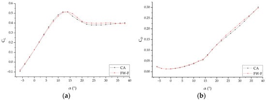
Figure 10.
Comparison of CL and CD of the front wing between Front-Wing-Fuselage (FW-F) model and Complete Aircraft (CA) model: (a) CL curves; (b) CD curves.
The CL and CD of the rear wing are shown in Figure 11. The trends of the CL and CD for the rear wing in the RW-F model and CA model show significant differences. This indicates that the rear wing is substantially influenced by the front wing. In the RW-F model, the critical angle of attack for the CL of the rear wing is 12°. Compared to the RW-F model, the critical angle of attack for the CL of the rear wing in the CA model increases to 14°, and the maximum CL is significantly reduced, resulting in a lower CL. Before reaching the critical angle of attack, the slope of the CL curve for the rear wing in the CA model is noticeably smaller. The loss in the rear wing’s CL is shown in Figure 11a.
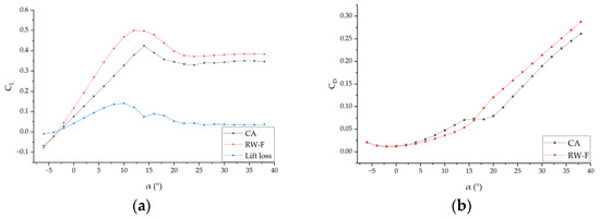
Figure 11.
Comparison of CL and CD of the rear wing between RW-F model and CA model: (a) CL curves and lift loss; (b) CD curves.
The lift loss first increases and then decreases, reaching its maximum at a 10° angle of attack and accounting for 30% of the lift value in the RW-F model. Due to the aerodynamic interference of the front wing on the rear wing, the CD of the rear wing increases before a 16° angle of attack and decreases after an 18° angle of attack. It can be concluded that, before a 16° angle of attack, the aerodynamic interference of the front wing on the rear wing increases the rear wing’s drag, while, after an 18° angle of attack, this interference reduces the rear wing’s drag.
The variation in the front wing’s L/D with the angle of attack is shown in Figure 12a. Compared to the FW-F model, the L/D of the front wing in the CA model slightly decreases overall, but the trend remains the same. Between 2°and 12°angles of attack, the lift and drag coefficients of the two models are similar. However, due to the extremely low drag coefficients (ranging from 0 to 0.05), minor discrepancies cause significant fluctuations in the L/D comparison.
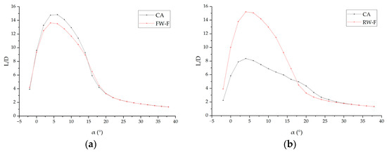
Figure 12.
(a) Comparison of L/D of the front wing between FW-F model and CA model; (b) Comparison of L/D of the rear wing between RW-F model and CA model.
The variation in the rear wing’s L/D with the angle of attack is shown in Figure 12b. Compared to the RW-F model, the L/D of the rear wing in the CA model is significantly reduced, and the trend undergoes a substantial change. Instead of the traditional smooth convex curve typical of a wing lift-to-drag ratio, the curve becomes irregular, indicating that the aerodynamic interference from the front wing has a significant impact on the rear wing’s L/D.
3.3.2. Flow Field Analysis
The aerodynamic data indicates that, in the tandem-wing configuration studied in this paper, the aerodynamic interference of the rear wing on the front wing is negligible and significantly smaller than that of the front wing on the rear wing. Therefore, the subsequent flow field analysis will primarily focus on investigating the aerodynamic interference of the front wing on the rear wing.
To visually examine the aerodynamic interference of the front wing on the rear wing in this tandem configuration, a comparative analysis of streamline patterns and velocity contours between the CA model and the RW-F model was conducted. A detailed analysis of the rear wing’s pressure coefficient (CP) distribution will be presented in the following section.
As shown in Figure 13, the left side displays cross-sections at Y = 0.65 m for the CA model, while the right side shows the RW-F model. From top to bottom, the figure presents streamline patterns and velocity contours at angles of attack from 10° to 22°. When airflow passes the front wing, velocity vectors change significantly near the wing surface but remain relatively unchanged farther away. Comparing the left and right sides reveals that, at smaller angles of attack, airflow above the front wing’s upper surface accelerates over the rear wing, effectively reducing its angle of attack. As the angle of attack increases within a certain range, the airflow adhering to the upper surface of the front wing exhibits progressively stronger interaction with the rear wing, leading to a continuous enhancement of aerodynamic interference effects on the rear wing.
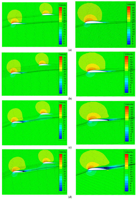
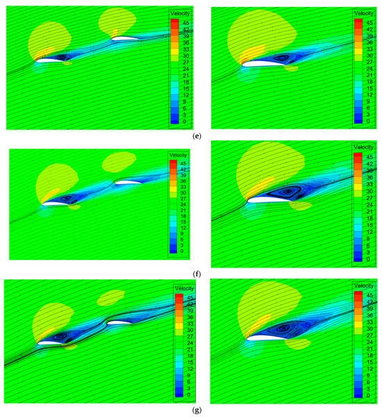
Figure 13.
Comparison of velocity contours and streamlines between CA model (left) and RW-F model (right), and angles of attack are as follows: (a) α = 10°; (b) α = 12°; (c) α = 14°; (d) α = 16°; (e) α = 18°; (f) α = 20°; (g) α = 22°.
Figure 13a–g demonstrate that, from 10° to 22° angles of attack, the front wing’s upper surface maintains higher flow velocity than the rear wing, while its lower surface shows lower velocity, resulting in significantly greater lift generation on the front wing. Starting from the 14° angle of attack, turbulent low-velocity airflow from the front wing’s trailing edge begins affecting the rear wing’s leading edge. By the 18° angle of attack, a pronounced low-velocity region forms at the rear wing’s leading edge, causing anomalous changes in the rear wing’s CD between 14 and 20° angles of attack, where CD growth slows or stalls (Figure 11b).
The front wing reaches CL,max at an approximately 13° angle of attack, while minor separation vortices appear at 12° (Figure 13b), showing slight trailing-edge separation while the rear wing remains attached. The rear wing’s critical angle occurs at 14° (Figure 11a) but without significant trailing-edge separation. Trailing-edge separation vortices on the rear wing first emerge at a 22° angle of attack (Figure 13g).
3.3.3. Pressure Coefficient Distribution on the Rear Wing
The spanwise sections of the rear wing for both the RW-F model and CA model are selected as shown in Figure 14. At a 10° angle of attack, the rear wing experiences maximum lift loss (Figure 11a), with the pressure coefficient (CP) distributions on the upper and lower surfaces presented in Figure 15. It can be observed that, without interference from the front wing, CP distribution of the rear wing is nearly unaffected by the fuselage and wingtip plates. CP distribution of CA model is shown in Figure 15b, revealing smaller lift near the wingtip plates. This indicates that the aerodynamic interference of the front wing on the rear wing also varies spanwise, with greater lift loss occurring closer to the wingtip.
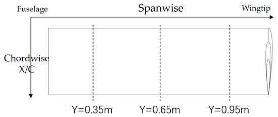
Figure 14.
Selected cross-section position.
Figure 15.
The pressure coefficient (CP) distributions on the upper and lower surfaces of the rear wing at 10° angle of attack for different models: (a) Fuselage + rear wing. (b) Complete aircraft.
The comparison of CP distributions at different spanwise sections of the rear wing between the RW-F model and CA model is shown in Figure 16. The results show that the front wing’s interference affects the rear wing in two aspects: first, CP in the negative pressure region near the leading edge of the rear wing’s upper surface increases significantly; second, CP in the extensive positive pressure region on the lower surface decreases to zero, resulting in a significant contraction of the positive pressure zone. These pressure changes on the wing surfaces clearly account for the lift loss observed on the rear wing in the CA model.
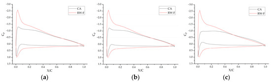
Figure 16.
Comparison of CP distributions of the rear wings between the RW-F model and CA model at different spanwise sections: (a) Y = 0.35 m; (b) Y = 0.65 m; (c) Y = 0.95 m.
3.4. Influence of Propellers on Aerodynamic Characteristics of Tandem Tilt-Wing Configuration
To investigate the influence of propellers on overall aerodynamic characteristics during cruise flights across varying angles of attack, a comparative analysis was conducted between propeller-driven configuration (PDC) and propeller-off configuration (POF). In PDC, the propeller rotational speed is set to 6000 rpm.
CL and CD variations in PDC with an angle of attack are shown in Figure 17. As shown in Figure 17a, the front wing of the PDC exhibits a significantly higher CL compared to the rear wing, with the CL slope of the front wing also surpassing that of the rear wing. It is evident from Figure 17b that, with increasing angles of attack, the CD of both the front wing, rear wing, and the total aircraft demonstrates a characteristic trend of initial decrease followed by subsequent increase. The rear wing consistently maintains a lower CD than the front wing throughout the tested angle-of-attack range. Compared to the POF, the CD of the front wing and rear wing in PDC changes more regularly with the angle of attack, and the difference between the front wing and rear wing increases steadily.
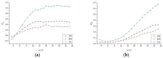
Figure 17.
CL and CD for each component of the propeller-driven configuration during the cruise flight: (a) CL curves; (b) CD curves.
Compared to POF, component-specific aerodynamic comparisons are shown in Figure 18. Figure 18a indicates that, beyond the critical angle of attack, the propeller action increases the front wing’s CL and maintains it at higher values, eliminating the stall-induced sharp drop in CL. Figure 18c reveals that propellers reduce the rear wing’s maximum CL, increase their critical angle of attack, and cause non-monotonic variations in CL with the angle of attack. As depicted in Figure 18e, between 6° and 16° angles of attack, the total aircraft CL decreases compared to POF, and, beyond the 16° angle of attack, the total CL increases without stall-induced collapse.
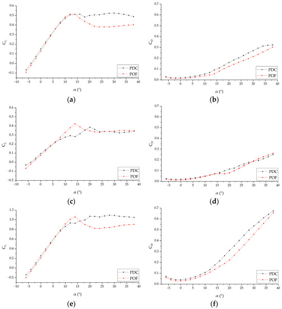
Figure 18.
Comparison of CL and CD for each component of the aircraft during the tilt transition conditions between PDC and POF: (a) CL of the front wing; (b) CD of the front wing; (c) CL of the rear wing; (d) CD of the rear wing; (e) CL of the total aircraft; (f) CD of the total aircraft.
The propeller’s effects on the CD are shown in Figure 18b,d,f: propeller action increases the front wing’s CD; the rear wing’s CD increases overall with a smoother curve progression; and the total aircraft CD increases across all angles.
4. Aerodynamic Characteristics of Tandem Tilt-Wing Aircraft in Transitional States
4.1. Computational Model Setup
To examine the aerodynamic coupling effects between the front wing and rear wing during tilt transition, three computational models were established, as shown in Figure 6: FW-F model, RW-F model, and CA model. The analysis considered wing tilt angles ranging from 0° (horizontal) to 90° (vertical) at 10° intervals. Flow field simulation and analysis were sequentially performed for each model, with a simplified workflow diagram presented in Figure 19.
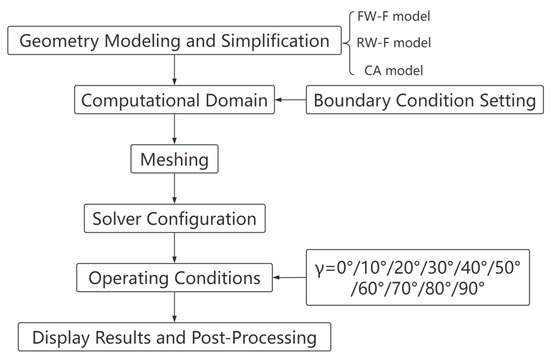
Figure 19.
Flowchart of flow field simulation analysis in transitional states.
In the CA model, the aerodynamic force coefficients of the front wing, rear wing, and total aircraft were compared, along with their variation patterns with wing tilt angles. At the same time, comparative assessments were performed by analyzing the FW-F model against CA model data and similarly comparing the RW-F model with CA model data. This methodology enables systematic investigation of both the front wing’s influence on the rear wing and the reciprocal interference effects of the rear wing on the front wing.
4.2. Aerodynamic Characteristics of Tandem-Wing Configuration
The lift and drag characteristics of the propeller-off model under tilt transition conditions at 10° intervals are shown in Figure 20.
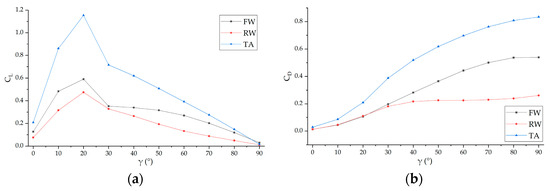
Figure 20.
CL and CD for each component of the propeller-off aircraft during the tilt transition conditions: (a) CL curves; (b) CD curves.
As depicted in Figure 20a, the CL trends of the front wing, rear wing, and the total aircraft are consistent, and CL initially increases then decreases as the wing tilt angle varies from 0° (horizontal) to 90° (vertical), approaching zero at 90° tilt angle. The CL,max of the front wing, rear wing, and the total aircraft occurs at 20° tilt angle.
Figure 20b presents the drag characteristics. The CD of the front wing, rear wing, and the total aircraft exhibit continuous growth throughout the 0–90° tilt transition. Notably, the front wing maintains a higher CD than the rear wing, with this differential progressively increasing. Beyond a 40° tilt angle, the rear wing’s CD shows minimal variation. Between 60° and 90° wing tilt angles, the CD of the front wing consistently reaches twice that of the rear wing.
L/D characteristics for each component of the propeller-off aircraft model are presented in Figure 21. As the wing tilt angle increases from 0° to 90°, the L/D of the front wing, rear wing, and the total aircraft exhibit similar trends: their L/D initially increases then decreases, ultimately approaching zero, with peak values achieved at 10° tilt angle, and the L/D of the front wing is 60% higher than that of the rear wing at this condition.
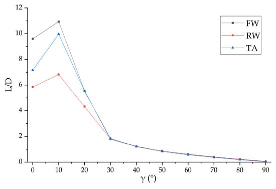
Figure 21.
L/D for each component of the propeller-off aircraft during the tilt transition conditions.
4.3. Analysis of Aerodynamic Coupling Effects in Tandem-Wing Configuration
4.3.1. Aerodynamic Data Analysis
Figure 22 compares the CL and CD of the front wing between the FW-F model and CA model. As the wing tilt angle increases, the front wing’s CL initially increases and then decreases, while the CD continuously increases. Compared to the FW-F model, the CL in CA shows a slight increase at a 10° wing tilt angle, a significant increase at 20°, and an overall slight decrease in the 30–90° tilt angle range, while the CD exhibits a minor reduction across the entire tilt range.
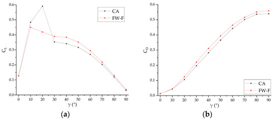
Figure 22.
Comparison of CL and CD of the front wing between FW-F model and CA model: (a) CL curves; (b) CD curves.
A comparison of the CL and CD of the rear wing between the RW-F model and CA model is shown in Figure 23. Significant discrepancies in CL, CD, and their trends with the wing tilt angle confirm substantial aerodynamic interference from the front wing on the rear wing. As the wing tilt angle increases, the front wing’s CL initially increases and then decreases, while its CD continuously increases.
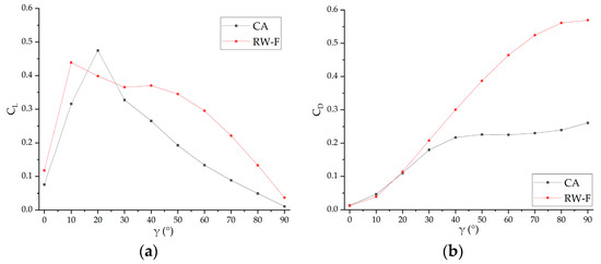
Figure 23.
Comparison of CL and CD of the rear wing between the RW-F model and CA model: (a) CL curves; (b) CD curves.
As shown in Figure 23a, the maximum CL of the rear wing in the RW-F model occurs at a 10° wing tilt angle, whereas, in the CA model, the rear wing’s maximum CL shifts to a 20° wing tilt angle. Overall, due to aerodynamic interference from the front wing, the rear wing’s CL in the CA model is significantly reduced at all tilt angles except 20°. Figure 23b shows that the rear wing’s CD increases with tilt angle in both models, but a critical divergence emerges beyond the 30° tilt angle: the CD of the RW-F model continues to increase at a steady rate, while the CD growth rate in the CA model plummets to near-zero, resulting in CD values significantly lower than those of the RW-F model at high tilt angles (40–90°).
Aerodynamic data analysis reveals that, unlike in cruise flights, both front-to-rear and rear-to-front wing aerodynamic interference are significant during tilt transition. Figure 24 quantifies the bidirectional lift loss and drag variation (penalty/reduction). The lift loss variations in both the front and rear wings are shown in Figure 24a: at a 10° wing tilt angle, the rear wing’s influence increases the front wing’s CL slightly, while the front wing’s aerodynamic interference reduces the rear wing’s CL by 28%; at a 20° tilt angle, mutual aerodynamic interactions between the front and rear wing enhance the CL for both with greater amplification observed on the front wing, and the CL of the front wing increased by 41%, while that of the rear wing increased by 19%; between 30 and 90° tilt angles, bidirectional interference causes lift reduction for both wings, with the rear wing exhibiting more significant degradation. The drag variations in both front and rear wings are shown in Figure 24b. The rear wing’s influence induces a minor drag reduction on the front wing with nearly constant magnitude across angles. Between 30 and 90° tilt angles, the front wing’s aerodynamic interference causes significant drag reduction on the rear wing, with the reduction amplitude progressively increasing as the tilt angle grows. At an 80° wing tilt angle, the CD loss of the rear wing reaches its peak, with a magnitude of up to 57%.
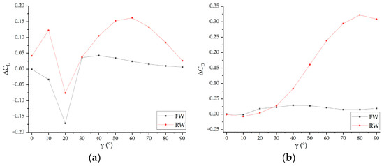
Figure 24.
Comparison of lift loss and drag penalty between CA model front wing vs. FW-F model and CA model rear wing vs. RW-F model: (a) lift loss curves; (b) drag penalty curves.
4.3.2. Flow Field Analysis
To visually study the aerodynamic coupling effects between the front and rear wings in the tandem-wing configuration during tilt transition, a comparative analysis of aerodynamic characteristics at the Y = 0.65 m flow field cross-section for three configurations was conducted: CA model, FW-F model, and RW-F model. In the streamline and pressure contour diagrams below, the left panel shows the front wing flow field of the FW-F model, the middle panel displays the coupled flow field of front and rear wings in the CA model, and the right panel presents the rear wing flow field of the RW-F model.
Figure 25a shows the streamlines and pressure contours at a 10° tilt angle. Compared to the FW-F model and RW-F model, in the CA model, the coupled flow field of both front and rear wings creates an integrated low-pressure region on their upper surfaces. Additionally, the pressure in the low-pressure region on the upper surface of the rear wing increases. The front wing’s lower surface exhibits a slight high-pressure enhancement, while the rear wing’s lower surface shows a significant high-pressure region reduction, leading to increased lift for the front wing and decreased lift for the rear wing.
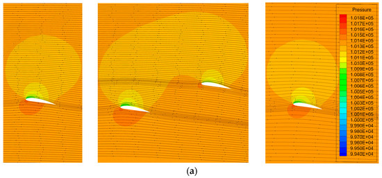
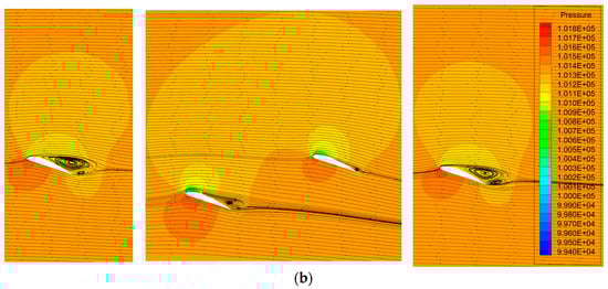
Figure 25.
The streamlines and pressure contours at wing tilt angles of 10° and 20°: (a) 10° wing tilt angle; (b) 20° wing tilt angle.
Figure 25b demonstrates that, at a 20° tilt angle, compared to the FW-F model and RW-F model, the coupled flow field forms a continuous low-pressure zone over both wings’ upper surfaces in the CA model, significantly reducing leading-edge pressure and weakening trailing-edge separation vortices. The diminished low-pressure region at the rear wing’s lower trailing edge, combined with enhanced high pressure on the front wing’s lower surface, explains why the front wing’s lift increases substantially more than the rear wing’s lift at this tilt angle.
Figure 26 reveals the aerodynamic coupling between the front and rear wings at 60° and 80° tilt angles. Compared to the FW-F model, the front wing experiences a slight reduction in pressure on the upper surface in the CA model, resulting in a minor decrease in its lift coefficient (Figure 24a). Compared to the RW-F model, the rear wing in the CA model shows a significant decrease in pressure on its lower surface, which explains its substantial reductions in both lift and drag coefficients (Figure 24). The interacting flow field between the wings creates a mutual interference zone, where the rear wing resides predominantly within the front wing’s turbulent wake. This positioning of the rear wing partially suppresses the development of the front wing’s separation vortices.
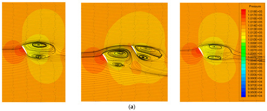
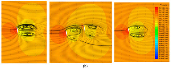
Figure 26.
The streamlines and pressure contours at wing tilt angles of 60° and 80°: (a) 60° wing tilt angle; (b) 80° wing tilt angle.
4.4. Influence of Propellers on Aerodynamic Characteristics of Tandem Tilt-Wing Configuration
To investigate the influence of propellers on overall aerodynamic characteristics during tilt transition at different wing tilt angles, a comparative analysis was conducted between PDC and POF. In PDC, the propeller rotational speed is set to 6000 rpm.
CL and CD variations in the propeller-driven configuration with a tilt angle are shown in Figure 27. The aerodynamic coefficients vary with wing tilt angles as follows: as the wing tilt angle increases, the CL of front wing, rear wing, and total aircraft first increase and then decrease, with the CL of front wing consistently exceeding that of rear wing. The CD of the front wing and total aircraft continuously increase, while the CD of the rear wing follows a complex trend—first increasing, then decreasing, and subsequently increasing again.
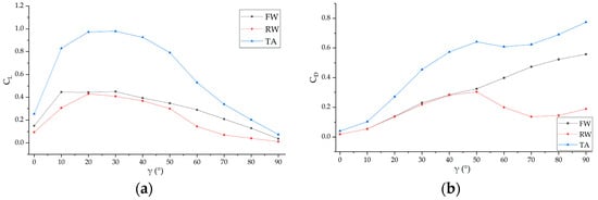
Figure 27.
CL and CD for each component of the propeller-driven configuration during tilt transition conditions: (a) CL curves; (b) CD curves.
The variations of CL with a wing tilt angle for each component of the aircraft between PDC and POF are shown in Figure 28a,c,e. Compared to POF, the propeller’s influence reduces the CL,max of the front wing, rear wing, and total aircraft. The propeller’s effect on the CL is most pronounced between 10 and 30° tilt angles. From 30° to 60° tilt angles, the propeller’s influence increases the CL of the front wing, rear wing, and total aircraft, bringing them closer to the values observed in the 10–30° tilt angle range and resulting in smoother lift coefficient variations. The CL curves of the POF exhibit a sharp peak followed by rapid decay, while the PDC shows smoother variations with gentler transitions.
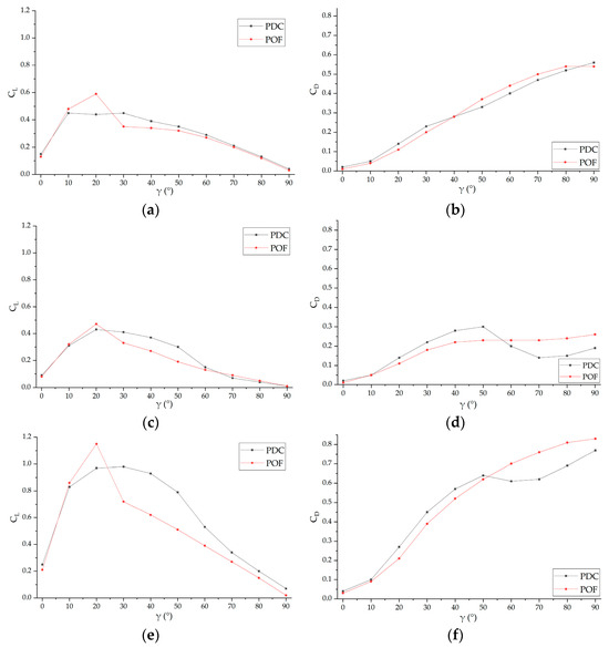
Figure 28.
Comparison of CL and CD for each component of the aircraft during tilt transition conditions between PDC and POF: (a) CL of the front wing; (b) CD of the front wing; (c) CL of the rear wing; (d) CD of the rear wing; (e) CL of the total aircraft; (f) CD of the total aircraft.
As shown in Figure 28e, the CL of the total aircraft in the POF peaks sharply at 20° tilt angle before decreasing rapidly between 10 and 30° tilt angles. In contrast, the PDC achieves its maximum CL at 30° tilt angle, primarily due to propeller-induced modifications to fuselage lift. The fuselage CL (Figure 29a) demonstrates significant enhancement in the PDC starting from a 20° tilt angle compared to the POF.
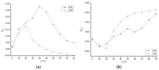
Figure 29.
Comparison of CL and CD for fuselage of the aircraft during tilt transition conditions between PDC and POF: (a) CL of the fuselage; (b) CD of the fuselage.
The CD variations with wing tilt angles for both configurations are shown in Figure 28b,d,f. At smaller tilt angles, the PDC exhibits higher CD for the front wing, rear wing, and total aircraft compared to the POF. At larger tilt angles, the propeller reduces CD across all components, creating more complex variation patterns. The total aircraft CD inherits characteristics from both wings, with pronounced differences in rear wing CD between configurations leading to a distinct drag reduction phase in the PDC. Additionally, the propeller reduces the fuselage CD across the entire tilt range compared to POF (Figure 29b).
5. Conclusions
Numerical simulations were conducted to analyze the strongly coupled nonlinear aerodynamic characteristics of the designed tandem tilt-wing UAV during cruise flight and tilt transition. By computing the variations in lift/drag coefficients of each component with an angle of attack and wing tilt angle, combined with velocity contours, pressure coefficient distributions, and pressure contours, the aerodynamic mechanisms were analyzed.
During both the level flight and tilt transition, aerodynamic interference from the front wing on the rear wing consistently exceeds the rear wing’s influence on the front wing, resulting in significantly lower lift and drag coefficients for the rear wing. Consequently, the aircraft’s aerodynamic center shifts forward, detrimentally impacting static stability. To mitigate this, the design of tandem tilt-wing aircraft necessitates a proportionally larger rear wing area.
During the level flight, aerodynamic coupling between the wings primarily manifests as the front wing’s influence on the rear wing (with negligible reverse effects), as evidenced by lift/drag coefficient comparisons. During tilt transition, bidirectional interference exists between the wings as tilt angle changes, but the front wing’s influence on the rear wing remains significantly stronger.
Aerodynamic interference between the wings does not always cause lift loss. During tilt transition simulations, lift coefficients increase at specific tilt angles where baseline lift coefficients are already high, posing greater challenges for practical tilt-wing UAV control.
During tilt transition, the propeller reduces the maximum lift coefficients of the main lift surfaces of the aircraft but generally increases their lift coefficients across tilt angles, resulting in smoother lift coefficient variations that enhance flight stability and controllability.
Author Contributions
Conceptualization, B.X., G.T. and L.J.; methodology, B.X.; software, B.X. and L.J.; validation, B.X., G.T. and L.J.; formal analysis, B.X.; investigation, B.X.; resources, J.C. and J.Z.; data curation, B.X.; writing—original draft preparation, B.X.; writing—review and editing, B.X. and J.C.; visualization, J.Z.; supervision, B.X.; project administration, G.T.; funding acquisition, G.T. All authors have read and agreed to the published version of the manuscript.
Funding
This research received no external funding.
Data Availability Statement
The authors confirm that the data supporting the findings of this study are available within this article.
Conflicts of Interest
The authors declare no conflicts of interest.
Abbreviations
The following abbreviations are used in this manuscript:
| eVTOL | Electric Vertical Take-Off and Landing |
| UAV | Unmanned Aerial Vehicle |
| CFD | Computational Fluid Dynamics |
| MRF | Multiple Reference Frame |
| NS | Navier–Stokes |
| RANS | Reynolds-Averaged Navier–Stokes |
| URANS | Unsteady Reynolds-Averaged Navier–Stokes |
| α | Angle of Attack |
| γ | Wing Angle |
| CL | Lift Coefficient, Normal Force/Q*S |
| CD | Drag Coefficient, Axial Force/Q*S |
| L/D | Lift-to-Drag Ratio |
| n | Propeller Speed |
| η | Propeller efficiency |
| FW | Front Wing |
| RW | Rear Wing |
| TA | Total Aircraft |
| CA | Complete Aircraft |
| POF | Propeller-Off Configuration |
| PDC | Propeller-Driven Configuration |
References
- Wang, G.; Wu, Z. Comprehensive Analysis of Overall Configuration and Control Strategies for VTOL UAVs. Aircr. Des. 2006, 26, 25–30. [Google Scholar]
- Cai, J.; Cai, R. Development History and Key Technologies of the V-22 Osprey Tiltrotor Aircraft. Aeronaut. Sci. Technol. 2013, 11–14. [Google Scholar]
- Mu, Z.; Cheng, W.; Song, G. Application of Electric Propulsion Technology in Aviation. Aeronaut. Sci. Technol. 2019, 30, 30–35. [Google Scholar]
- Kong, X.; Zhang, Z.; Lu, J.; Li, J.; Yu, L. Review of Distributed Electric Propulsion Aircraft Power Systems. Acta Aeronaut. Astronaut. Sin. 2018, 39, 46–62. [Google Scholar]
- Karthik, A.; Chiniwar, D.S.; Das, M.; Prabhu, P.; Mulimani, P.A.; Samanth, K.; Naik, N. Electric propulsion for fixed wing aircrafts–a review on classifications, designs, and challenges. Eng. Sci. 2021, 16, 129–145. [Google Scholar] [CrossRef]
- Figat, M.; Kwiek, A. Analysis of longitudinal dynamic stability of tandem wing aircraft. Aircr. Eng. Aerosp. Technol. 2023, 95, 1411–1422. [Google Scholar] [CrossRef]
- Rhodes, M.D.; Selberg, B.P. Benefits of dual wings over single wings for high-performance business airplanes. J. Aircr. 1984, 21, 116–127. [Google Scholar] [CrossRef]
- Zhao, J. Research on Structural Design and Control Methods for Tilt-Wing Aircraft. Master’s Thesis, Shandong University, Jinan, China, 2022. [Google Scholar]
- Stokkermans, T.C.A.; Usai, D.; Sinnige, T.; Veldhuis, L.L.M. Aerodynamic Interaction Effects Between Propellers in Typical eVTOL Vehicle Configurations. J. Aircr. 2021, 58, 815–833. [Google Scholar] [CrossRef]
- Zanotti, A.; Velo, A.; Pepe, C.; Savino, A.; Grassi, D.; Riccobene, L. Aerodynamic interaction between tandem propellers in eVTOL transition flight configurations. Aerosp. Sci. Technol. 2024, 147, 17. [Google Scholar] [CrossRef]
- Geuther, S.C.; North, D.D.; Busan, R.C. Investigation of a Tandem Tilt-Wing VTOL Aircraft in the NASA Langley 12-Foot Low-Speed Tunnel; NASA Langley Research Center: Hampton, VA, USA, 2020.
- Liu, F.; Ma, D.; Luo, J. Wind Tunnel Experimental Study on Transition Characteristics of a Small Multi-Rotor Tilt-Wing Aircraft. Helicopter Tech. 2023, 215, 29–33. [Google Scholar]
- Johnson, W. Calculation of the aerodynamic behavior of the tilt rotor aeroacoustic model (TRAM) in the DNW. In Proceedings of the American Helicopter Society 57th Annual Forum, Washington, DC, USA, 9–11 May 2001. [Google Scholar]
- Johnson, W. Influence of wake models on calculated tiltrotor aerodynamics. In Proceedings of the American Helicopter Society Aerodynamics, Acoustics, and Test and Evaluation Technical Specialist Meeting Proceedings, San Francisco, CA, USA, 23–25 January 2002. [Google Scholar]
- Sheng, C.H.; Narramore, J.C. Computational Simulation and Analysis of Bell Boeing Quad Tiltrotor Aero Interaction. J. Am. Helicopter Soc. 2009, 54, 15. [Google Scholar] [CrossRef]
- Gupta, V.; Baeder, J. Investigation of quad tiltrotor aerodynamics in forward flight using CFD. In Proceedings of the 20th AIAA Applied Aerodynamics Conference, St. Louis, MO, USA, 24–26 June 2002; p. 2812. [Google Scholar]
- Shinozuka, A.; Taniguchi, S.; Yasue, K.; Fukuchi, R.; Oyama, A. Aerodynamic Analysis of Tandem Tilt-Wing eVTOL Aircraft in Cruise and Transition Flight. In Proceedings of the AIAA SciTech Forum, Orlando, FL, USA, 8–12 January 2024. [Google Scholar]
- Huang, Q.J.; He, G.Y.; Jia, J.K.; Hong, Z.L.; Yu, F. Numerical Simulation on Aerodynamic Characteristics of Transition Section of Tilt-Wing Aircraft. Aerospace 2024, 11, 283. [Google Scholar] [CrossRef]
- Li, P.; Zhao, Q.; Wang, B. High-Efficiency Predefined Boundary Motion Overset Grid Method for Rotor CFD Simulations. Acta Aerodyn. Sin. 2015, 33, 747–756. [Google Scholar]
- Li, P.; Zhao, Q. CFD Analysis of Aerodynamic Characteristics for Tiltrotor Aircraft in Typical Flight Conditions. J. Aerosp. Power 2016, 31, 421–431. [Google Scholar]
- Li, P.; Zhao, Q.; Yin, J.; Zhu, Q.; Wang, B. A Novel Overset Grid Method for Aerodynamic Analysis of Tiltrotor Aircraft. J. Aero-Space Power 2017, 32, 2145–2159. [Google Scholar]
- Wang, Z.; Yang, Y.; Zhao, H.; Zhao, J. Numerical Simulation of Tilting Wing and Rotor UAV During Transition Flight. Mod. Def. Technol. 2024, 52, 9. [Google Scholar]
- Wang, Y.; He, G.; Wang, Q. Aerodynamic Analysis and Optimization of Tilt-Wing UAV During Return Transition Phase. Eng. Sci. Technol. 2022, 22, 9848–9856. [Google Scholar]
- Pengqian, Y.; Yutong, C.; Junhui, L.; Jiehao, Y.; Jiayuan, S.; Shijun, S. Study on High-Angle-of-Attack Aerodynamics and Controllability of Tandem-Wing Cargo UAV. Acta Aeronaut. Astronaut. Sin. 2025, 46, 131056. [Google Scholar]
- Liu, P. Aerodynamics; Springer: Beijing, China, 2021. [Google Scholar]
- Jones, W.P.; Launder, B.E. The prediction of laminarization with a two-equation model of turbulence. Int. J. Heat Transf. 1972, 15, 301–314. [Google Scholar] [CrossRef]
- Wilcox, D.C. Reassessment of the scale-determining equation for advanced turbulence models. AIAA J. 1988, 26, 1299–1310. [Google Scholar] [CrossRef]
- Spalart, P.; Allmaras, S. A one-equation turbulence model for aerodynamic flows. In Proceedings of the 30th Aerospace Sciences Meeting and Exhibit, Reno, NV, USA, 6–9 January 1992; p. 439. [Google Scholar]
- Menter, F.R. Two-equation eddy-viscosity turbulence models for engineering applications. AIAA J. 1994, 32, 1598–1605. [Google Scholar] [CrossRef]
- Chen, T. Aerodynamic Characteristics Analysis and Design Study of Quad-Tiltrotor Aircraft. Master’s Thesis, Nanjing University of Aeronautics and Astronautics, Nanjing, China, 2018. [Google Scholar]
- Gudmundsson, S. General Aviation Aircraft Design: Applied Methods and Procedures; Butterworth-Heinemann: Oxford, UK, 2013. [Google Scholar]
Disclaimer/Publisher’s Note: The statements, opinions and data contained in all publications are solely those of the individual author(s) and contributor(s) and not of MDPI and/or the editor(s). MDPI and/or the editor(s) disclaim responsibility for any injury to people or property resulting from any ideas, methods, instructions or products referred to in the content. |
© 2025 by the authors. Licensee MDPI, Basel, Switzerland. This article is an open access article distributed under the terms and conditions of the Creative Commons Attribution (CC BY) license (https://creativecommons.org/licenses/by/4.0/).