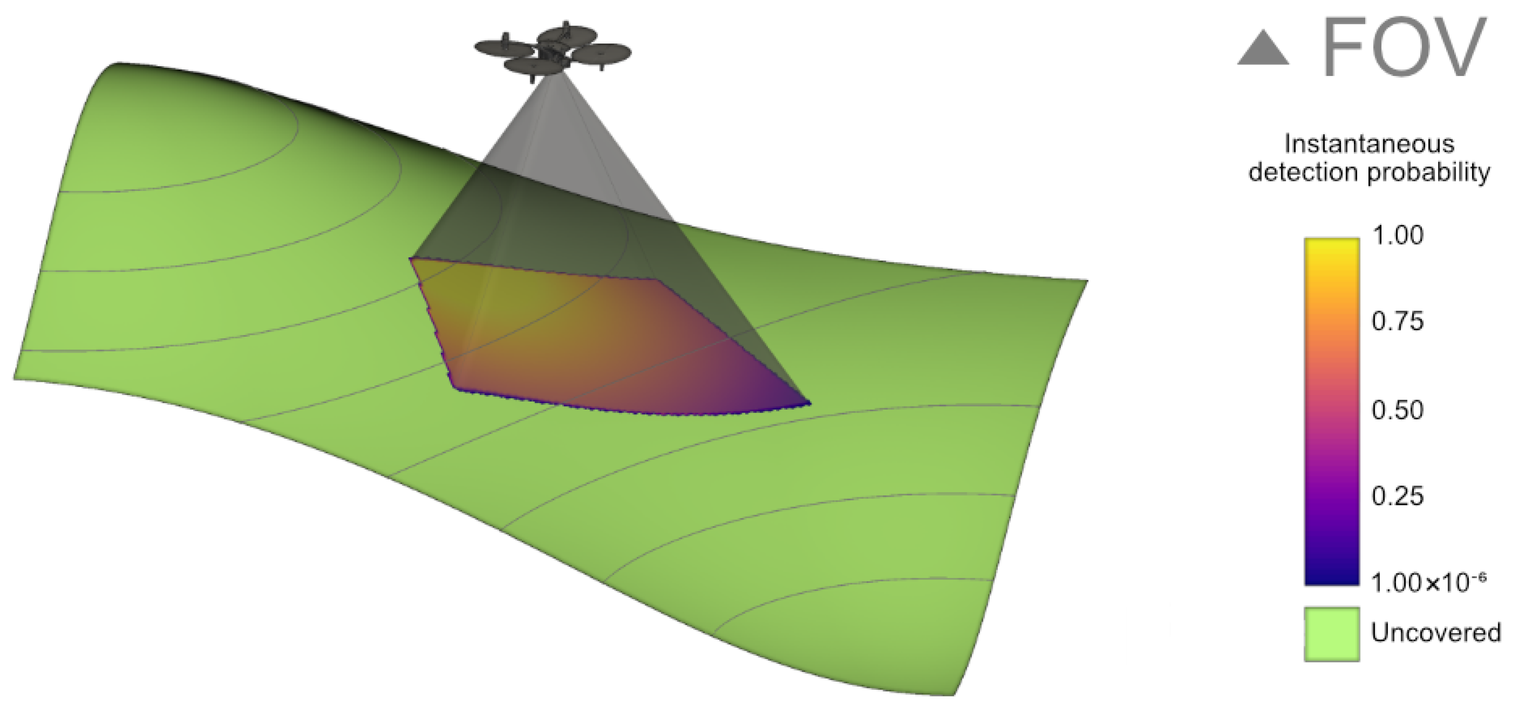
Figure 1.
The FOV of a single UAV is represented by a semi-transparent pyramid. The detection probability in the UAV’s FOV is shown using a gradient that increases the detection probability for points closer to the UAV’s orthogonal view according to the sensing model, while the undetectable points are represented in green color.
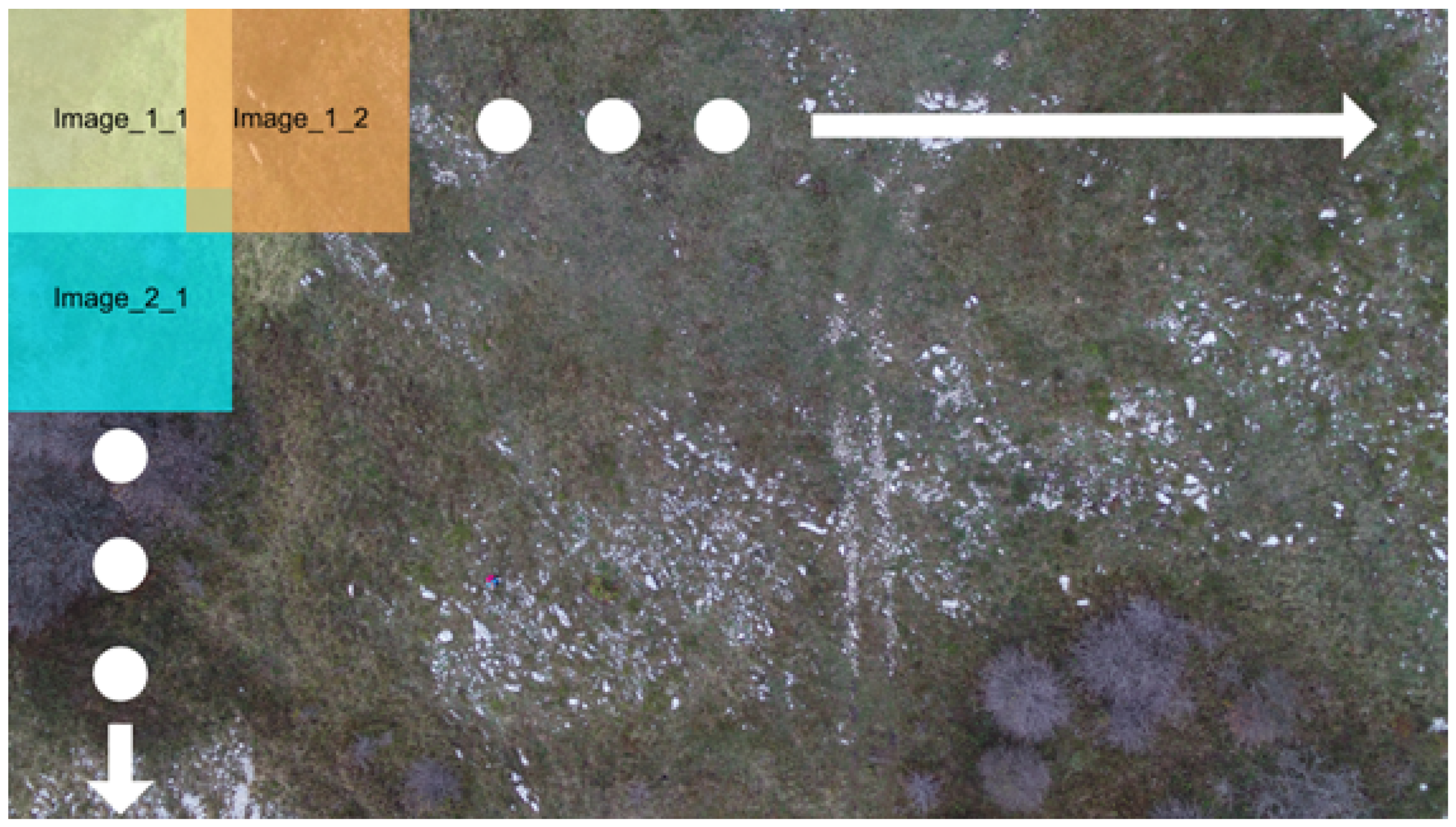
Figure 2.
The tiling method used to divide original sized images into images of 512 × 512 pixels. The overlap ensures more context being available in the newly created dataset.
Figure 2.
The tiling method used to divide original sized images into images of 512 × 512 pixels. The overlap ensures more context being available in the newly created dataset.
Figure 3.
Distribution of images captured by each camera categorized by GSD. The majority of the images have a GSD ranging from 1.0 to 2.5 cm/px indicating high spatial resolution across most images. This initial distribution is directly relevant to the main experiment where the flight regime is optimized resulting in a similar distribution of having most images in the range of 1.5–3.0 cm/px.
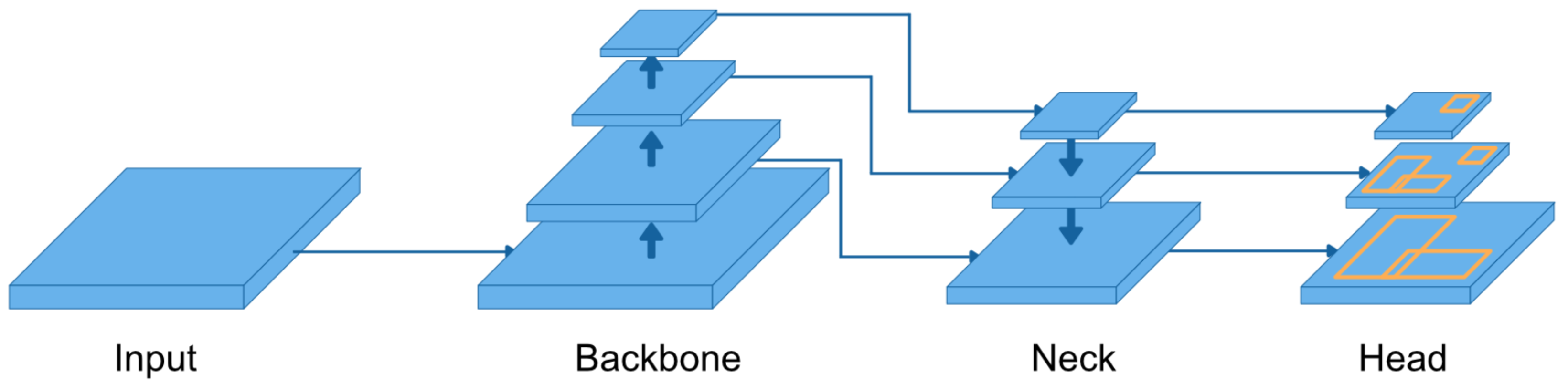
Figure 4.
Simplified YOLO architecture. The input data is sent to the backbone which extracts image features by propagating it through multiple layers. The neck is enhancing the created feature maps by using different scales. The head is predicting bounding boxes.
Figure 4.
Simplified YOLO architecture. The input data is sent to the backbone which extracts image features by propagating it through multiple layers. The neck is enhancing the created feature maps by using different scales. The head is predicting bounding boxes.
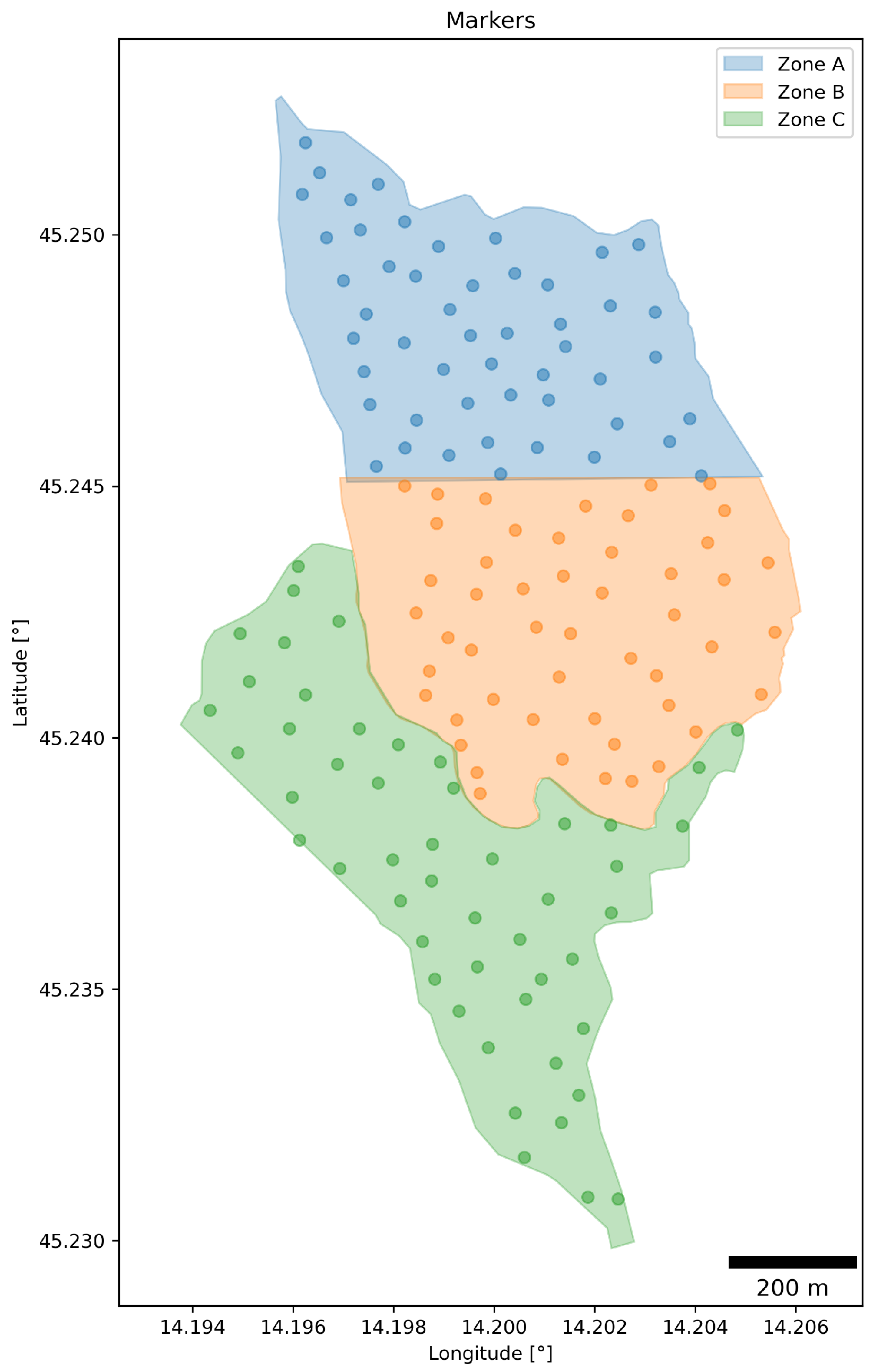
Figure 5.
Three zones and their corresponding markers. Each zone contains 50 markers for the treasure hunt ensuring a uniform distribution of participants during the search experiment.
Figure 5.
Three zones and their corresponding markers. Each zone contains 50 markers for the treasure hunt ensuring a uniform distribution of participants during the search experiment.
Figure 6.
The information flier containing the map of the search area and zones in (a) as well as all important information for the participants and the log section in (b). The original version of the flier is in Croatian, but for the purpose of including this flier in the paper, it has been translated into English.
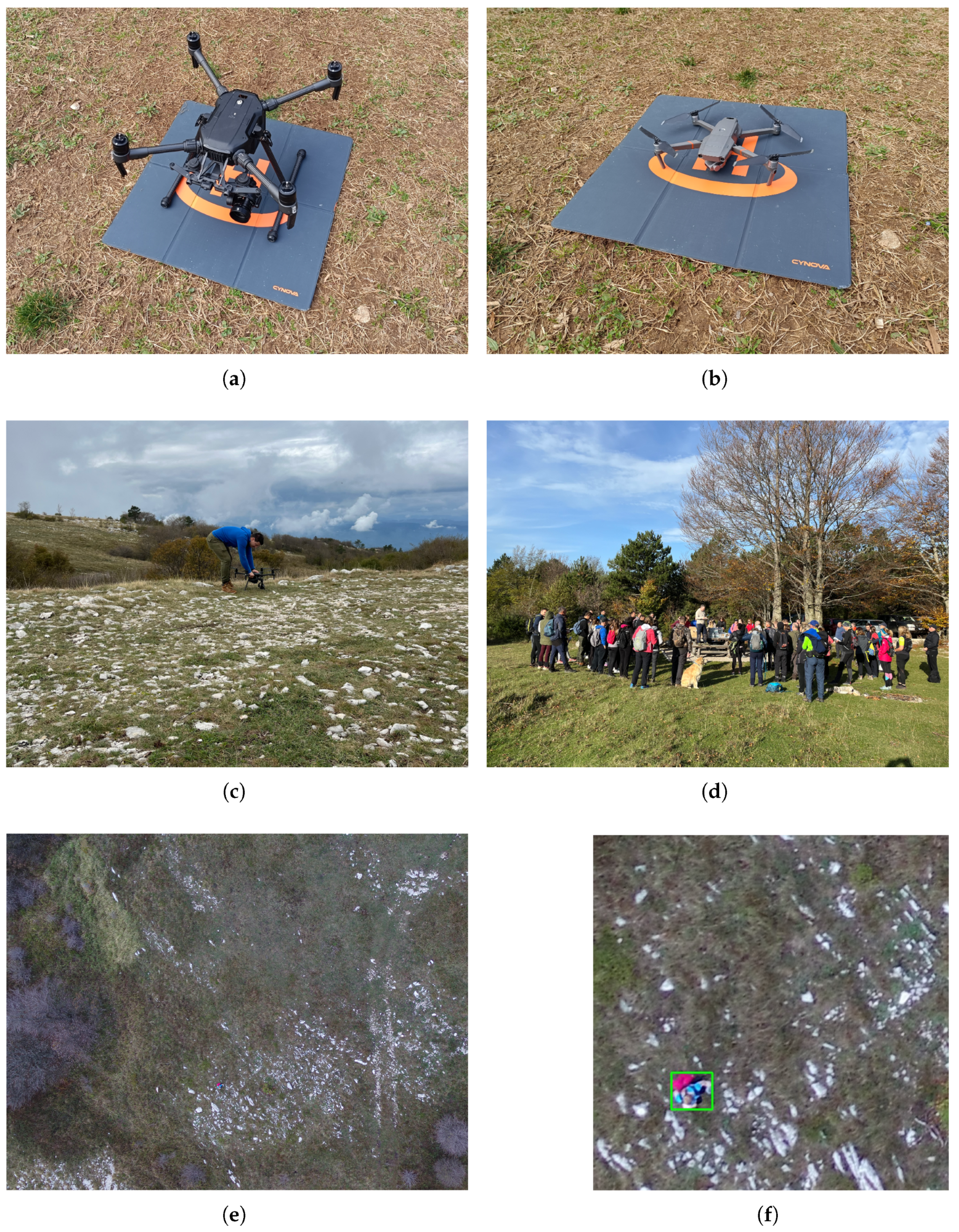
Figure 7.
Scenes from conducting the experiment. Subfigure (a) shows the Matrice 210 v2 UAV and Subfigure (b) displays the Mavic 2 Enterprise Dual UAV. Subfigure (c) illustrates the preparation to begin the mission at the home point of each flight. In (d) the participants are depicted while the introduction speech has been given. Subfigure (e) shows one example of UAV images and (f) presents one tile of the image containing a detected participant.
Figure 8.
All flight trajectories of all search missions. (a) visualizes the flights conducted during Search mission 1 consisting of flights 1, 2, and 3. In (b) the trajectory of Search mission 2 is displayed. (c) illustrates the flight trajectory of Search mission 3. (d) combines the trajectories of all search missions.
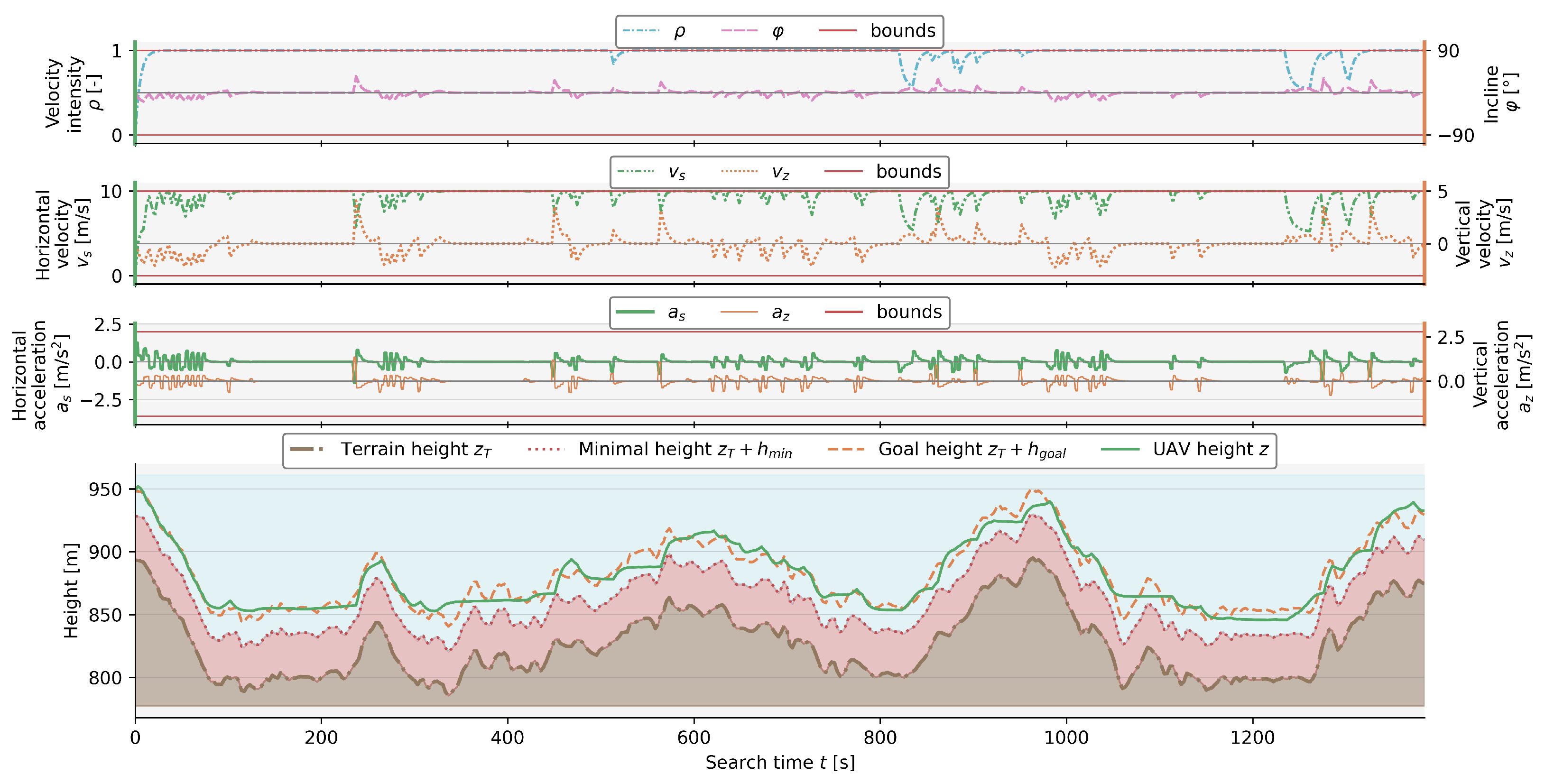
Figure 9.
The first flight of Search mission 1 with a MPC horizon length of 15 s during a 1400 s flight. The UAV’s velocity and acceleration is inside the set constraints. The goal flight height is set to 55 m with the UAV maximizing the flight velocity, while minimizing the flight height resulting in a smoother line.
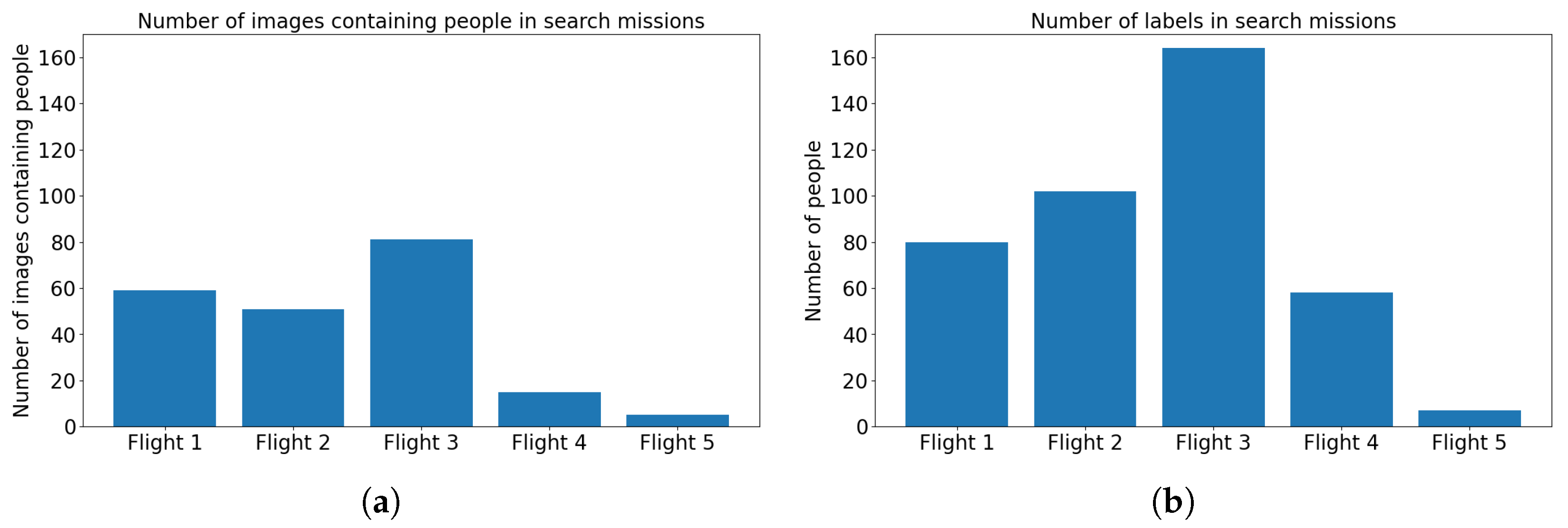
Figure 10.
Number of images containing people and number of labels in each search mission. (a) represents the number of images with labels and (b) is showing the number of labels in all UAV flights. It can be seen that the Flight 3 contains most images as well as labels. Flight 1 contains more images with labels than Flight 2, but less labels. Even though Flight 5 consisted of only one zone, it has the lowest number of images containing people and labels.
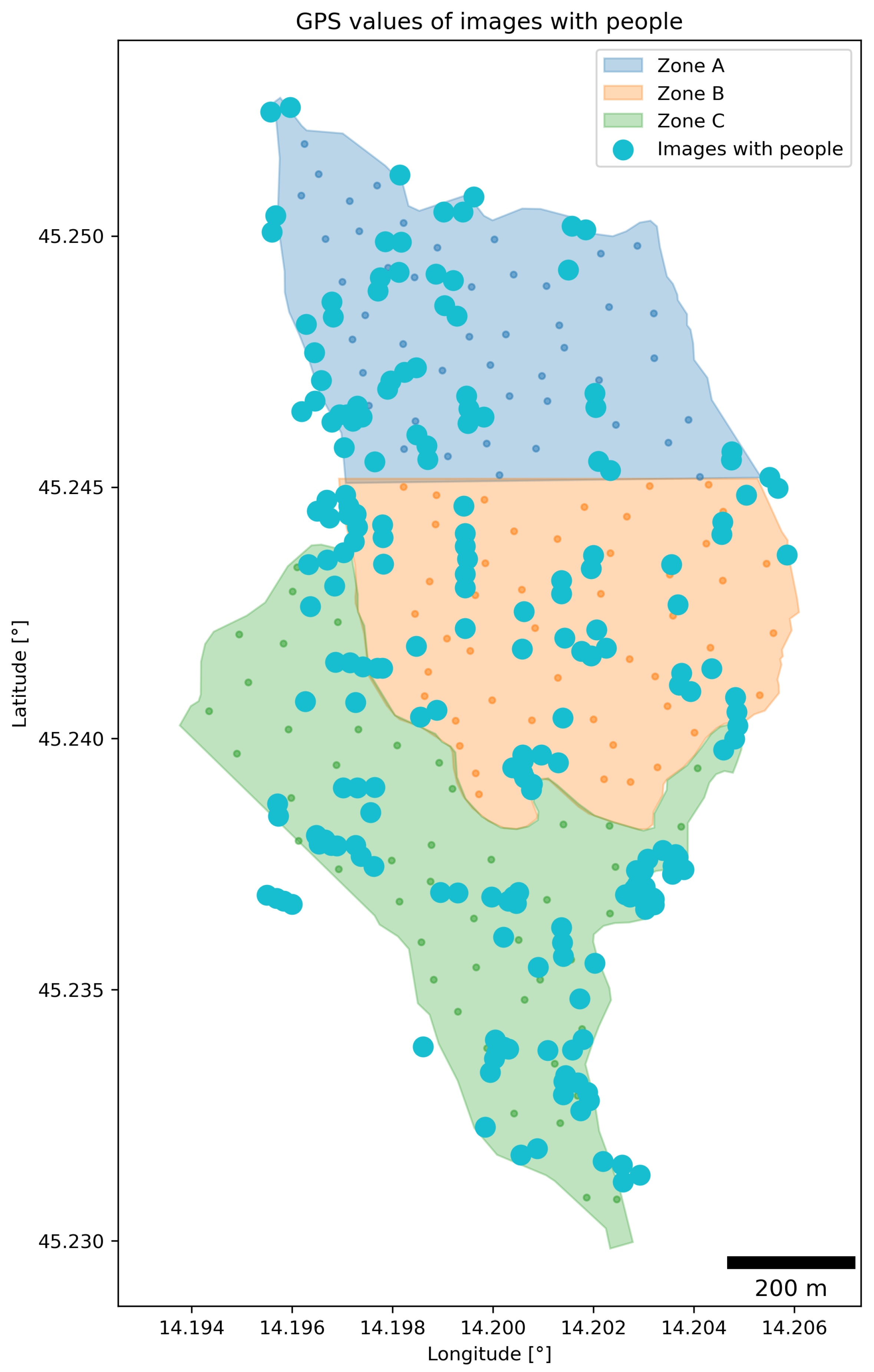
Figure 11.
All images containing people and their locations. The UAV flight zone is larger than the defined zones containing markers. Most people were detected in the location of the starting point. This is expected since two UAV flight operators were in this location at all times and took images at the UAV flight start and end of each flight.
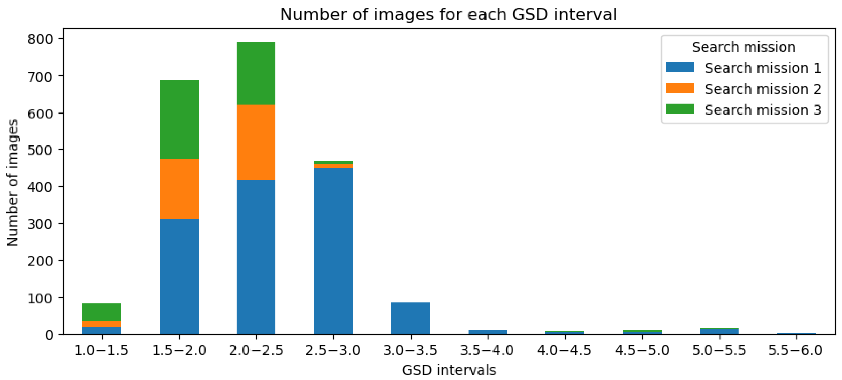
Figure 12.
Number of images in each GSD interval for each Mission. Search mission 1 was the longest one and consisted of three flights generating the largest amount of images for most GSD intervals. It is important to note that this represents all images, meaning that not only images with labels are considered, but also images without them.
Figure 13.
Recall of images created as tiles of images containing people. The initial experiment was operated manually with no height optimization resulting in more GSD intervals than the autonomously operated missions in the search experiment. Nevertheless, it can be seen that the missions’ recall follows the general trend of the recall declining with higher GSDs.
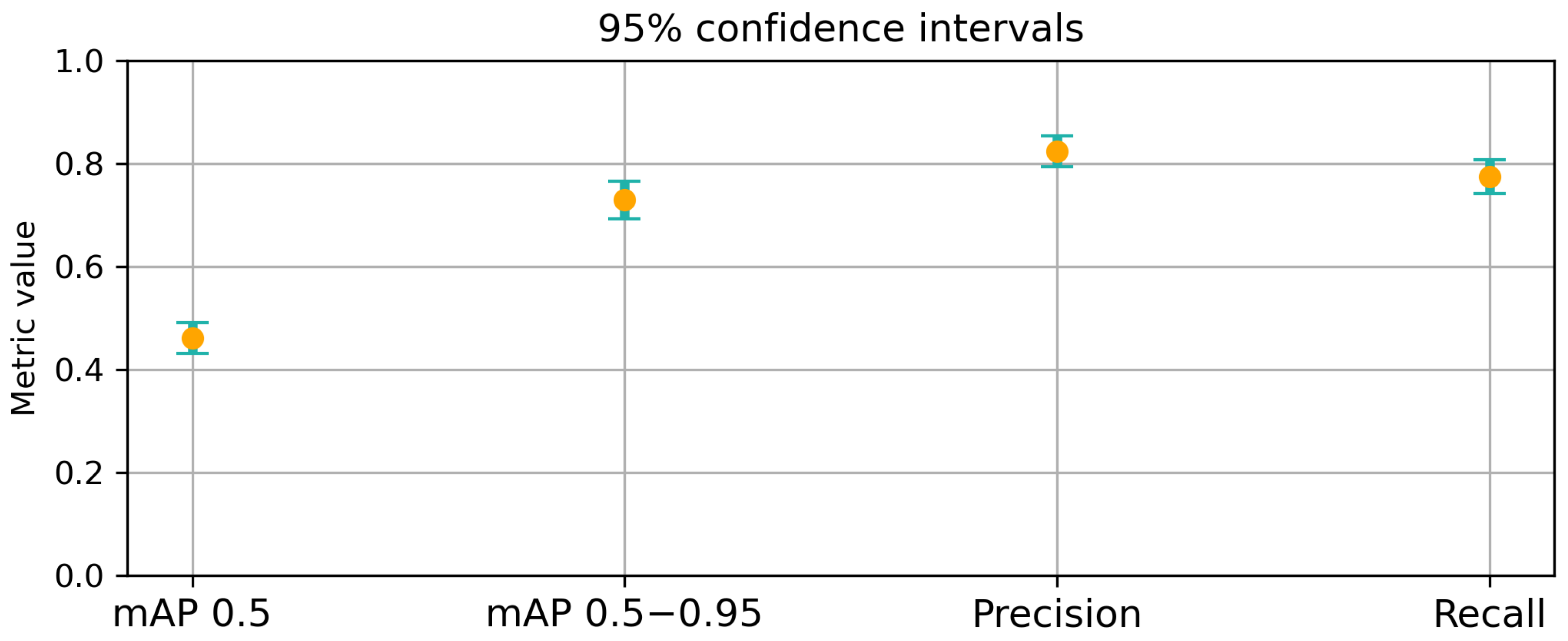
Figure 14.
Bootstrapped 95% confidence intervals for detection performance metrics, including mAP 0.5, mAP 0.5–0.95, precision, and recall. To estimate the variability of the metrics, 100 images were randomly sampled from the dataset and this process was repeated 200 times. The results illustrate the variability and robustness of the detection system using repeated sampling, confirming the consistency.
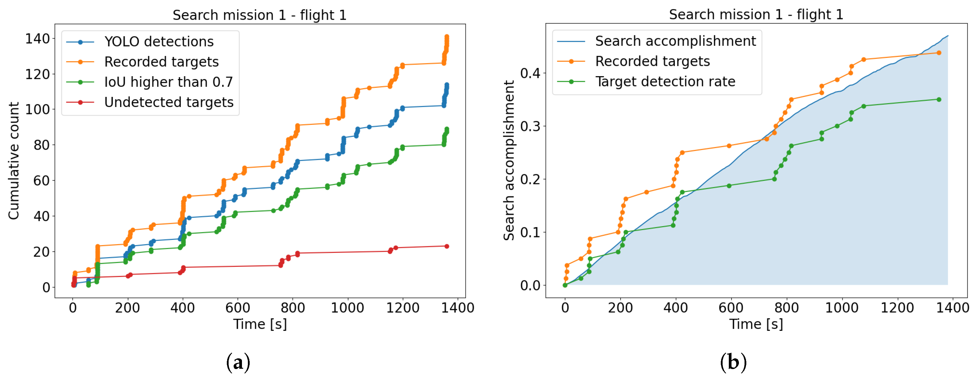
Figure 15.
The detections and search accomplishment of the first flight in Search mission 1. (a) displays the recorded targets meaning the manually labeled individuals, the YOLO detections of detections with a confidence score higher than 0.5, the detections with an intersection over union (IoU) higher than 0.7 and the undetected targets. In (b) the predicted search accomplishment is shown in blue, the recorded manual identifications obtained by images taken in the experiment are illustrated in orange, while the YOLO detection rate is presented in green. The points indicate timestamps of images detecting an individual for the first time.
Figure 16.
Confusion matrices for Search mission 1 in (a) and 2 in (b). Most ground truth labels have been detected, while the background area in the ground truth could only be mistakenly predicted as a person causing the maximum percentage being detected as persons. It is important to note that the Search mission 3 only contained seven labels, making the results not relevant.
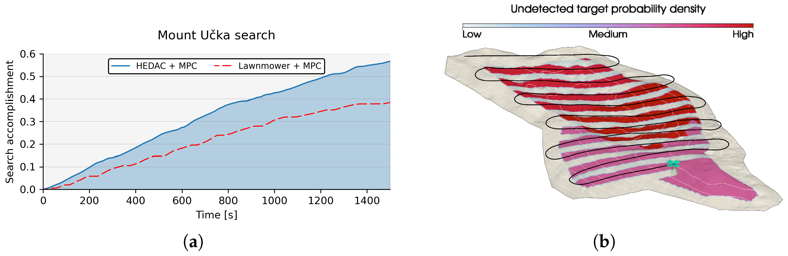
Figure 17.
Comparison of the search accomplishment between the used HEDAC-MPC framework and a traditional lawnmower coverage method in simulation shown in (a). The HEDAC-MPC approach demonstrates more effective coverage by prioritizing high-probability regions based on the probabilistic model, resulting in faster and more efficient detection of targets. In (b) the simulated lawnmower trajectory is visualized.
Table 1.
Recall for each GSD group in the initial experiment.
Table 1.
Recall for each GSD group in the initial experiment.
| GSD | Recall |
|---|
| 0.5–1.0 | 0.95 |
| 1.0–1.5 | 0.977 |
| 1.5–2.0 | 0.956 |
| 2.0–2.5 | 0.953 |
| 2.5–3.0 | 0.897 |
| 3.0–3.5 | 0.881 |
| 3.5–4.0 | 0.781 |
| 4.0–4.5 | 0.796 |
| 4.5–5.0 | 0.719 |
| 5.0–5.5 | 0.699 |
| 5.5–6.0 | 0.621 |
| 6.0–6.5 | 0.142 |
Table 2.
UAV specifications.
Table 2.
UAV specifications.
| UAV | Full Name | Unit | Matrice 210 v2 | Mavic 2
Enterprise Dual |
|---|
| Minimum incline angle | ° | −90 | −90 |
| Maximum incline angle | ° | 90 | 90 |
| Minimum horizontal velocity | m/s | 0 | 0 |
| Maximum horizontal velocity | m/s | 10 | 8 |
| Minimum vertical velocity | m/s | −3 | −2 |
| Maximum vertical velocity | m/s | 5 | 3 |
| Minimum horizontal acceleration | m/s2 | −3.6 | −3.6 |
| Maximum horizontal acceleration | m/s2 | 2 | 2 |
| Minimum vertical acceleration | m/s2 | −2 | −2 |
| Maximal vertical acceleration | m/s2 | 2.8 | 2.8 |
| Maximal angular velocity | °/s | 120 | 30 |
| MPC horizon timesteps (duration) | (s) | 5 (15) | 5 (15) |
Table 3.
Camera specifications.
Table 3.
Camera specifications.
| Camera | FOV c1 [°] | FOV c2 [°] | Resolution [px] |
|---|
| DJI Zenmuse X5S | 39.2 | 64.7 | 5280 × 2970 |
| DJI Zenmuse Z30 | 33.9 | 56.9 | 1920 × 1080 |
| Mavic 2 Enterprise Dual built-in camera | 57.58 | 72.5 | 4056 × 3040 |
Table 4.
Experiment setup settings.
Table 4.
Experiment setup settings.
| Flight | 1 | 2 | 3 | 4 | 5 |
|---|
| Search mission | Mission 1 | Mission 1 | Mission 1 | Mission 2 | Mission 3 |
| UAV | M210 | M210 | M210 | Mavic | M210 |
| Camera | X5S | X5S | Z30 | Mavic built-in camera | X5S |
| Min/goal altitude [m] | 35/55 | 55/75 | 35/75 | 35/55 | 35/55 |
| Zone | A, B, C | A, B, C | A, B, C | B, C | A |
| Start time | 11:15 | 11:44 | 12:13 | 12:40 | 13:02 |
| End time | 11:38 | 12:07 | 12:35 | 12:55 | 13:27 |
Table 5.
Specification of each zone.
Table 5.
Specification of each zone.
| Zone | Area [m2] | Num. Markers | Num. People |
|---|
| A | 432,734 | 50 | 25 |
| B | 470,233 | 50 | 27 |
| C | 613,709 | 50 | 26 |
Table 6.
Performance metrics for all five flights, illustrating the influence of camera quality, weather conditions, and the number of images containing people on detection outcomes. Flights 1 and 2 show the best performance, reflecting clearer image quality and minimal fog interference.
Table 6.
Performance metrics for all five flights, illustrating the influence of camera quality, weather conditions, and the number of images containing people on detection outcomes. Flights 1 and 2 show the best performance, reflecting clearer image quality and minimal fog interference.
| | Flight 1 | Flight 2 | Flight 3 | Flight 4 | Flight 5 |
|---|
| Precision | 0.82 | 0.85 | 0.42 | 0.56 | 0.68 |
| Recall | 0.62 | 0.74 | 0.16 | 0.43 | 0.59 |
| mAP 0.5 | 0.68 | 0.73 | 0.14 | 0.39 | 0.55 |
| mAP 0.5–0.95 | 0.44 | 0.42 | 0.09 | 0.20 | 0.49 |
Table 7.
Recall for each GSD group in all search missions.
Table 7.
Recall for each GSD group in all search missions.
| GSD | SM1 | SM2 | SM3 |
|---|
| 1.0–1.5 | 1 | | 1 |
| 1.5–2.0 | 0.71 | 0.51 | 0.67 |
| 2.0–2.5 | 0.68 | 0.37 | 0.38 |
| 2.5–3.0 | 0.80 | | |
| 3.0–3.5 | 0.37 | | |
Table 8.
Comparison of the performance between the YOLOv8l model pretrained on the COCO dataset and the YOLOv8l model additionally trained on our initial dataset. The results show a significant improvement in performance when the model is further trained on our data, highlighting the positive impact of domain-specific fine-tuning on the model’s accuracy and robustness.
| | | Our Model | YOLOv8l |
|---|
| |
GSD
|
SM1
|
SM2
|
SM3
|
SM1
|
SM2
|
SM3
|
|---|
| Precision | 1.0–1.5 | 0.98 | | 0.99 | 0.43 | | 0.11 |
| 1.5–2.0 | 0.88 | 0.83 | 0.28 | 0.54 | 0.24 | 1 |
| 2.0–2.5 | 0.76 | 0.53 | 0.64 | 0.46 | 0.13 | 0.02 |
| 2.5–3.0 | 0.84 | | | 0.40 | | |
| 3.0–3.5 | 0.62 | | | 0 | | |
| Recall | 1.0–1.5 | 1 | | 1 | 0.50 | | 1 |
| 1.5–2.0 | 0.71 | 0.51 | 0.67 | 0.39 | 0.71 | 0.64 |
| 2.0–2.5 | 0.68 | 0.37 | 0.38 | 0.22 | 0.51 | 0.38 |
| 2.5–3.0 | 0.80 | | | 0.17 | | |
| 3.0–3.5 | 0.37 | | | 0.11 | | |
| mAP 0.5 | 1.0–1.5 | 1 | | 1 | 0.47 | | 0.68 |
| 1.5–2.0 | 0.77 | 0.53 | 0.28 | 0.42 | 0.38 | 0.67 |
| 2.0–2.5 | 0.69 | 0.35 | 0.38 | 0.25 | 0.23 | 0.09 |
| 2.5–3.0 | 0.81 | | | 0.21 | | |
| 3.0–3.5 | 0.31 | | | 0 | | |
| mAP 0.5–0.95 | 1.0–1.5 | 0.80 | | 0.95 | 0.40 | | 0.67 |
| 1.5–2.0 | 0.52 | 0.23 | 0.21 | 0.29 | 0.18 | 0.44 |
| 2.0–2.5 | 0.41 | 0.19 | 0.31 | 0.17 | 0.16 | 0.08 |
| 2.5–3.0 | 0.48 | | | 0.15 | | |
| 3.0–3.5 | 0.15 | | | 0 | | |
| Overall precision | | | |
| Overall recall | | | |
Table 9.
Results of the correlation analysis between search accomplishment and detection rate. Pearson, Spearman, and Kendall’s tau correlation coefficients all indicate a strong positive relationship, with statistically significant p-values. The perfect Spearman rank and near-perfect and Kendall’s tau suggest the strictly increasing trend observed of the search accomplishment and detection rate in the search mission confirming that improvements in detection are closely associated with an enhanced search success.
| Test | Correlation | p-Value |
|---|
| Pearson | 0.99 | 1.05 |
| Spearman | 1 | 0 |
| Kendall tau | 1 | 1.19 |


