Pigeon-Inspired Transition Trajectory Optimization for Tilt-Rotor UAVs

Abstract

The continuous configuration changes and velocity variations of tilt-rotor UAVs during the transition phase pose significant challenges to flight safety. Hence, the transition phase trajectory must be specially designed. The transition corridor is an effective means of characterizing the controllable flight state and safe flight boundary of the tilt-rotor UAV transition phase. However, the conventional transition corridor is established based on the trim criterion, which cannot fully characterize the dynamic characteristics of the transition phase, resulting in deviations in the delineation of the flight boundary. This paper proposes a method that characterizes the dynamic transition corridor of a tilt-rotor UAV during the transition phase. A three-dimensional transition corridor considering the nacelle angle, velocity, and angle of attack is established by relaxing the force constraints and introducing angle of attack variables, allowing the dynamic characteristics of acceleration and deceleration in the transition phase to be characterized. On this basis, a transition trajectory optimization method based on the three-dimensional dynamic transition corridor is established using pigeon-inspired optimization with an objective that considers the smooth transition of tilt-rotor UAVs. Numerical simulations show that, compared with the transition trajectory obtained using a two-dimensional transition corridor, the proposed method ensures smoother changes in the velocity, nacelle angle, and expected angle of attack during the transition phase, resulting in stronger engineering practicality.

1. Introduction

As a new type of morphing aircraft integrating vertical take-off and landing with high-speed cruise capabilities, tilt-rotor UAVs have significant application potential in urban air traffic and inter-regional rapid transportation scenarios [1,2]. Advantages such as a large load capacity and high maneuverability also conform to the current development concept of the low-altitude economic industry and have broad developmental prospects [3,4,5]. However, modifying the configuration of tilt-rotor UAVs is relatively complicated [6,7,8]. When such aircraft transition from the hover phase to the cruise phase, the nacelle angle and flight speed undergo a wide range of changes, posing a great challenge to flight safety.

The transition corridor is an effective means of characterizing the controllable flight state and safe flight boundary of the tilt-rotor UAV transition phase. The transition corridor refers to the set of flight status points permitted for the tilt-rotor UAV during the transition phase. Various studies have explored the transition corridor of tilt-rotor UAVs. For instance, Chen et al. [9] calculated the low- and high-speed section boundaries of the transition corridor in accordance with the aircraft’s angle and power constraints. This approach enabled the determination of the two-dimensional transition corridor of the aircraft. Song et al. [10] constructed a transition corridor for a tilt-rotor UAV by prioritizing the low- and high-speed boundaries of the aircraft, and corrected the corridor boundaries using the power constraints of the aircraft. Zhang et al. [11] established a transition corridor for a tilt-rotor quadrotor aircraft by considering the limitations imposed by the stall of the wing, the dynamic stability, the flight power, and the blade loads. Yu [12] constructed a more stringent safety margin corridor based on the safety range of the state quantity. The transition corridors considered in the above studies are all trim transition corridors. The transition corridors considered in the above studies are all trim transition corridors. Every trim point within the corridor keeps the aerodynamic force and pitching moment of the tilt-rotor UAV unchanged. However, this method ignores the dynamic characteristics of the transition phase. Many studies have explored transition corridors that relax the trim conditions. May et al. [13] solved the transition corridor of a tilt-rotor UAV by combining the optimal control idea and reachable set theory for a longitudinal tilt-rotor UAV. Cheng et al. [14] designed a three-dimensional transition corridor for a tail-sitter aircraft, considering acceleration changes while maintaining a constant altitude. Although the above studies considered the effect of acceleration on the transition corridor, the direction of the flight velocity was not considered. Therefore, the solved corridors had relatively small ranges. The characterization of permissible states in the transition corridor requires further exploration.

The transition corridor represents the possible trajectory range of tilt-rotor UAVs. However, in actual flight, it is essential to select the most reasonable trajectory that ensures the robustness of the transition phase. Several scholars have researched methods of obtaining the transition trajectories of tilt-rotor UAVs based on transition corridors. For example, Xiao [15] calculated the flight state at typical nacelle angles in the transition phase and obtained the trajectory in segments according to the index requirements. Zuo [16] determined the transition trajectory of a tilt-rotor UAV based on the range of the transition corridor and the safety margin. In recent years, many researchers have used artificial intelligence to determine trajectories based on transition corridors. Jeongseok et al. [17] used a genetic algorithm and a stochastic gradient algorithm to optimize the transition trajectory using the minimum input as a metric. Hyun et al. [18] and Lyu et al. [19] employed an ant colony algorithm to optimize the trajectory of a box-wing aircraft and a tilt quad rotor. Zhang et al. [20] modified the A* algorithm to determine the globally optimal trajectory based on a bespoke path performance metric function. Chen et al. [21] used a method combining simulated annealing with a genetic algorithm to solve the optimal transition trajectory. The state points of the traditional transition corridor consider the balance of forces and moments at each static flight point. However, during actual flight, the aircraft’s velocity changes, and the two-dimensional transition corridor does not fully characterize all the information relevant to the transition phase. While some studies have considered the case of an aircraft accelerating horizontally, they typically do not incorporate the case of aircraft climbing or dropping significantly during the transition phase.

This paper proposes a characterization method for the transition corridor. The transition corridor is obtained by relaxing the trim conditions of the tilt-rotor UAV in the horizontal and vertical directions, considering the longitudinal acceleration. Based on this, a transition phase trajectory optimization method is established. The main contributions of this paper are as follows:

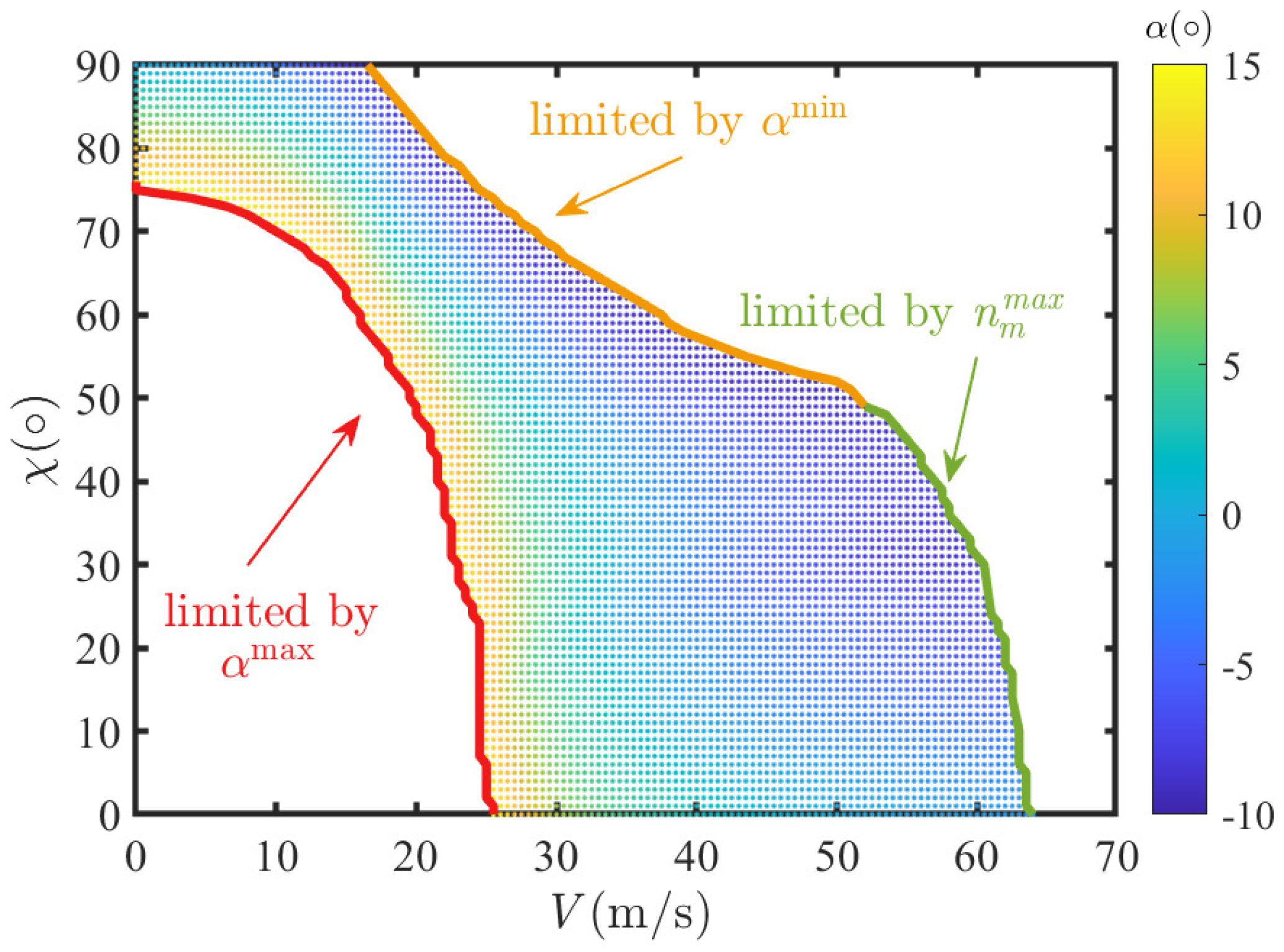
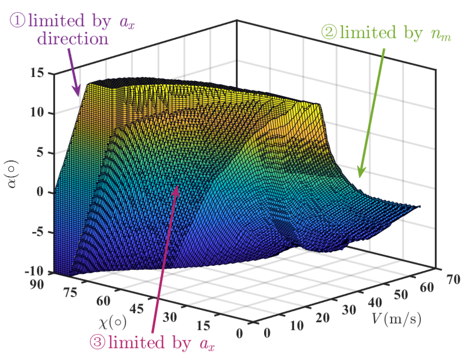
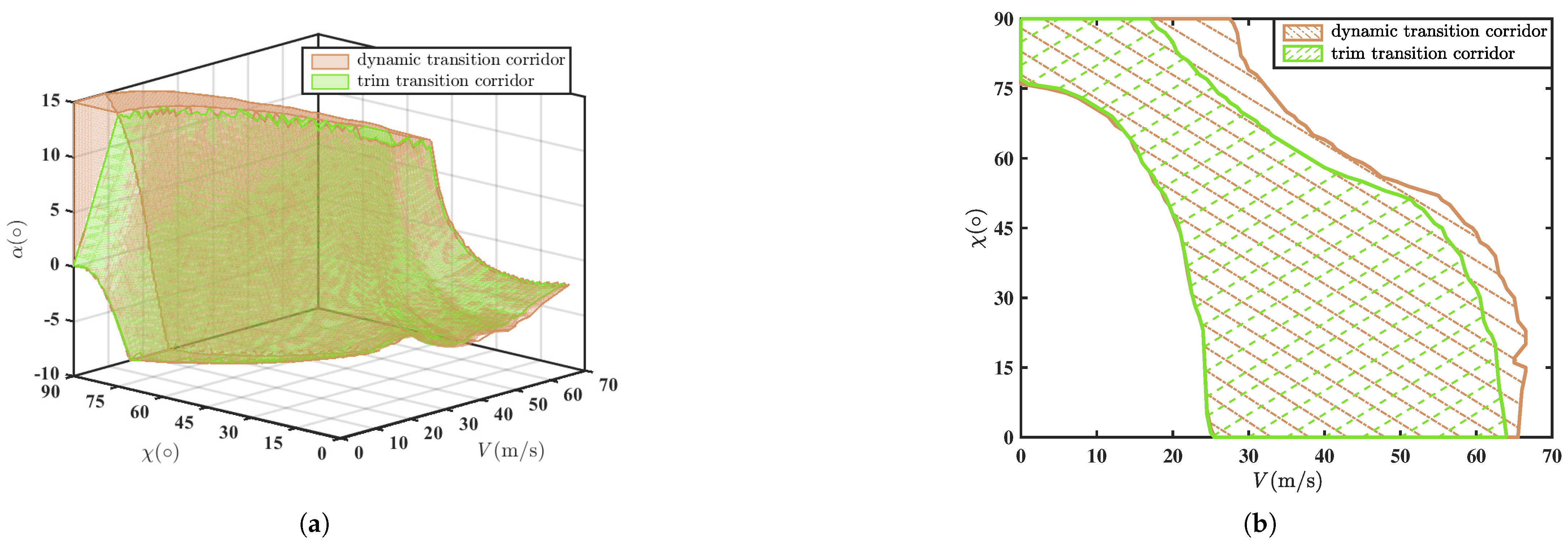
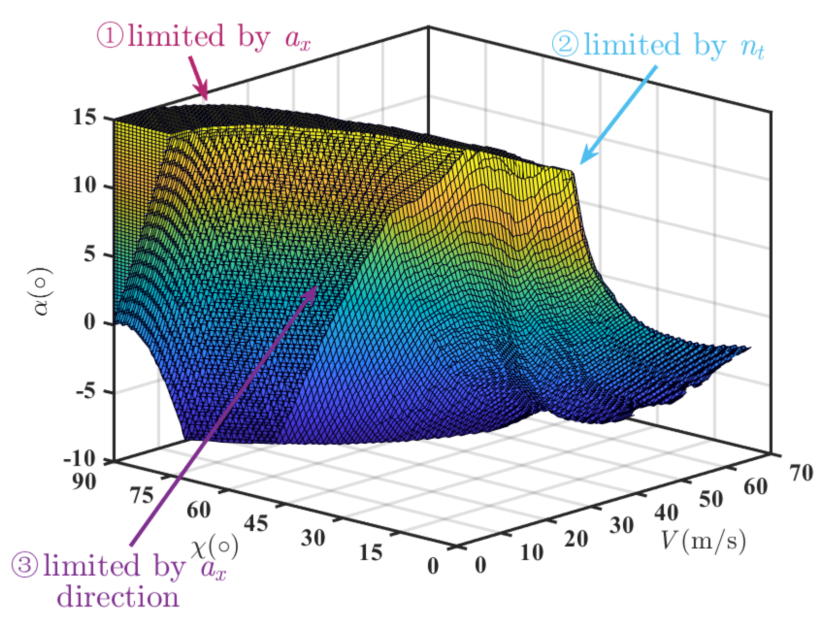
(1) Aiming at solving the problem whereby the two-dimensional trim transition corridor struggles to characterize the dynamic characteristics of the transition phase, resulting in deviations in the flight boundary characterization, a dynamic transition corridor characterization method for the transition phase of a tilt-rotor UAV is proposed. A three-dimensional transition corridor considering the nacelle angle, velocity, and angle of attack (AoA) is established to characterize the dynamic characteristics of acceleration and deceleration during the transition phase.

(2) Aiming at achieving the smooth transition of tilt-rotor UAVs, a transition trajectory optimization method based on the three-dimensional dynamic transition corridor is proposed. This method uses pigeon-inspired optimization (PIO) to accurately balance the nacelle angle, velocity, and AoA requirements in the transition from the hover phase to the cruise phase and vice versa.

The remainder of this paper is organized as follows. In Section 2, a three-degrees-of-freedom model of a tilt-rotor UAV is developed. Section 3 describes the trim transition corridor, followed by Section 4, which presents the three-dimensional dynamic transition corridor for the hover-to-cruise and cruise-to-hover phases. Section 5 applies the PIO algorithm to determine the trajectory during the transition phase. Finally, Section 6 concludes this paper.

2. Modeling of the Tilt-Rotor Aircraft

2.1. Tilt-Rotor UAV

The aircraft examined in this study is a novel class of tilt-rotor UAV as illustrated in Figure 1. The aircraft is equipped with four propellers. The propeller connected to the wing, which is called the main propeller, can be tilted 90° between vertical and horizontal positions. The propeller mounted on the upper extremity of the H-shaped tail is called the tail propeller. Tail propellers are used for attitude control and do not tilt. The outer wing of the nacelle is affixed to the nacelle itself. The outer wing-nacelle assemblies on both sides are kept in synchronized tilt, with the tilt axis positioned at the quarter chord of the wing. The main parameters of the prototype are listed in

Table 1. Main parameters of the tilt-rotor UAV.

Parameters	Values
Wing chord c (m)	$0.218$
Wing span b (m)	$2.317$
Single inner wing area $S_{iw}$ (${\mathrm{m}}^2$)	$0.141$
Single outer wing area $S_{ow}$ (${\mathrm{m}}^2$)	$0.090$
Main propeller diameter $r_m$ (m)	$1.015$
Tail propeller diameter $r_t$ (m)	$0.437$
Empennage area $S_t$ (${\mathrm{m}}^2$)	$0.145$

.

2.2. Three Degrees-of-Freedom Equation of the Tilt-Rotor UAV

The symmetry of the transverse–lateral motion of the tilt-rotor UAV during the transition phase means that only the longitudinal three-degrees-of-freedom model is considered. The tilt-rotor aircraft flies at a low speed and is subject to a small load during the transition phase; therefore, it can be assumed to be a rigid body. The model is characterized as follows:

$$\left\{\begin{array}{c}\dot{u}=-wq-gsin\theta +F_x^b/\phantom{F_x^{b}m}m\\ \dot{w}=uq+gcos\theta +F_z^b/\phantom{F_z^{b}m}m\\ \dot{\theta }=q\\ \dot{q}=M_y/\phantom{M_y{I}_{yy}}{I}_{yy}\end{array}\right.$$

(1)

where $F_x^b$ and $F_z^b$ are the x-axis and z-axis aerodynamic forces in the body axis system, u and w are the x-axis and z-axis velocities in the tilt-rotor’s body axis system, $M_y$ is the pitching moment, $\theta$ is the pitching angle, q is the pitch angular velocity, m is the mass of the aircraft, g is the acceleration due to gravity, and $I_{yy}$ is the moment of inertia of the tilt-rotor. The dynamic model of the tilt-rotor UAV is formulated through a component modeling method, wherein the aircraft is segmented into four components: propeller, wing, fuselage, and empennage. This segmentation leads to the following system of equations:

$$\left\{\begin{array}{c}{F}_x^b=F_{p\_x}^b+F_{w\_x}^b+F_{t\_x}^b+F_{f\_x}^b\hfill \\ F_z^b=F_{p\_z}^b+F_{w\_z}^b+F_{t\_z}^b+F_{f\_z}^b\hfill \\ M_y=M_p+M_w+M_t+M_f\hfill \end{array}\right.$$

(2)

where $F_{p\_x}^b$, $F_{w\_x}^b$, $F_{t\_x}^b$, and $F_{f\_x}^b$ represent the aerodynamic forces generated by the propeller, wing, empennage, and fuselage in the x-direction of the body axis; $F_{p\_z}^b$, $F_{w\_z}^b$, $F_{t\_z}^b$, and $F_{f\_z}^b$ represent the aerodynamic forces generated by the propeller, wing, empennage, and fuselage in the z-axis direction of the body axis; and $M_p$, $M_w$, $M_t$, and $M_f$ represent the pitching moment generated by the propeller, wing, empennage, and fuselage, respectively.

2.2.1. Propeller

The aerodynamic force generated by the propeller is given by the following equation:

$$\left\{\begin{array}{c}{F}_{p\_x}^b=(T_{main\_l}+T_{main\_r})\times cos\chi \hfill \\ F_{p\_z}^b=(T_{main\_l}+T_{main\_r})\times sin\chi +T_{tail\_l}+T_{tail\_r}\hfill \\ M_p=(T_{main\_l}+T_{main\_r})\times l_{main}+(T_{tail\_l}+T_{tail\_r})\ast l_{tail}\hfill \end{array}\right.$$

(3)

where $T_{main\_l}$, $T_{main\_r}$, $T_{tail\_l}$, and $T_{tail\_r}$ denote the thrust produced by four propellers; $\chi$ is the nacelle angle; and $l_{main}$ and $l_{tail}$ are the distances of the main propeller and the tail propeller from the center of gravity of the aircraft, respectively. The propeller’s thrust equations can be written as

$$T=C_T\rho {\left({\displaystyle \frac{n}{60}}\right)}^2{D}^4$$

(4)

where T is the thrust, $C_T$ is the pull force coefficient, n is the propeller speed in revolutions per minute (rpm), and $D_{*}$ is the propeller’s diameter. The propeller pulling force coefficient is modeled by the blade element method.

2.2.2. Wing

The wing dynamics of the tilt-rotor UAV are composed of two components: fixed wings and tilting wings. The combined forces and moments generated by the wings are expressed in the following equation:

$$\left\{\begin{array}{c}{L}_{w_f}=2C_L^{w_f}q{S}_{w_f}\hfill \\ L_{w_t}=2C_L^{w_t}q{S}_{w_t}\hfill \\ D_{w_f}=2C_D^{w_f}q{S}_{w_f}\hfill \\ D_{w_t}=2C_D^{w_t}q{S}_{w_t}\hfill \\ \left[\begin{array}{c}{F}_{w\_x}^b\\ F_{w\_z}^b\end{array}\right]=\left[\begin{array}{cc}sin\alpha & -cos\alpha \\ -cos\alpha & -sin\alpha \end{array}\right]\left[\begin{array}{c}{L}_{w_f}\\ D_{w_f}\end{array}\right]+\left[\begin{array}{cc}sin(\alpha +\chi )& -cos(\alpha +\chi )\\ -cos(\alpha +\chi )& -sin(\alpha +\chi )\end{array}\right]\left[\begin{array}{c}{L}_{w_t}\\ D_{w_t}\end{array}\right]\hfill \\ M_w=2\ast (C_m^{w_f}q{S}_{w_f}{c}_w+C_m^{w_t}q{S}_{w_t}{c}_w)+F_{w\_z}^b\times l_{wing}\hfill \end{array}\right.$$

(5)

where $L_{w_f}$ and $D_{w_f}$ are the lift and drag forces generated by the fixed wing, $L_{w_t}$ and $D_{w_t}$ are the lift and drag forces generated by the tilting wing, $C_L^{w_f}$ and $C_L^{w_t}$ are the lift coefficients of the fixed and tilting wings, $C_D^{w_f}$ and $C_D^{w_f}$ are the drag coefficients of the fixed and tilting wings, $C_m^{w_f}$ and $C_m^{w_f}$ are the pitching moment coefficients of the fixed and tilting wings, $S_{w_f}$ is the area of the fixed wing, $S_{w_t}$ is the area of the tilting wing, $\alpha$ is AoA, $\chi$ is the nacelle angle, q is the dynamic pressure of the aircraft, $c_w$ is the chord length of the wing, and $l_{w}ing$ is the distance of the quarter chord of the wing from the center of gravity of the aircraft. Neither the flaps nor the ailerons of the aircraft are deflected during the calculation of the transition corridor.

2.2.3. Empennage

The empennage of a tilt-rotor UAV is composed of two components: the elevator and the horizontal stabilizer. The aerodynamic forces generated by the empennage are as follows:

$$\left\{\begin{array}{c}{L}_t=C_L^{t}q{S}_t\hfill \\ D_t=C_D^{t}q{S}_t\hfill \\ \left[\begin{array}{c}{F}_{t\_x}^b\\ F_{t\_z}^b\end{array}\right]=\left[\begin{array}{cc}sin\alpha & -cos\alpha \\ -cos\alpha & -sin\alpha \end{array}\right]\left[\begin{array}{c}{L}_t\\ D_t\end{array}\right]\hfill \\ M_t=C_m^{t}q{S}_t{c}_t+F_{t\_z}^b\times l_e\hfill \end{array}\right.$$

(6)

where $L_t$ and $D_t$ are the lift and drag forces generated by the empennage, $C_L^t$ is the lift coefficient of the empennage, $C_D^t$ is the drag coefficient of the empennage, $C_m^t$ is the pitching moment coefficient of the empennage, $S_t$ is the area of the empennage, $c_t$ is the chord length of the empennage, and $l_e$ represents the distance of the quarter chord of the empennage relative to the center of gravity of the aircraft.

2.2.4. Fuselage

Tilt-rotor UAVs have a shuttle-shaped fuselage. To facilitate analysis of the aerodynamic forces generated by the fuselage, a calculation method analogous to that for the wing aerodynamic forces is used:

$$\left\{\begin{array}{c}{L}_f=C_L^{f}q{S}_f\hfill \\ D_f=C_D^{f}q{S}_f\hfill \\ \left[\begin{array}{c}{F}_{t\_x}^b\\ F_{t\_z}^b\end{array}\right]=\left[\begin{array}{cc}sin\alpha & -cos\alpha \\ -cos\alpha & -sin\alpha \end{array}\right]\left[\begin{array}{c}{L}_f\\ D_f\end{array}\right]\hfill \\ M_t=C_m^{t}q{S}_f{c}_w\hfill \end{array}\right.$$

(7)

where $L_f$ and $D_f$ are the fuselage’s lift and drag forces, $C_L^f$ is the lift coefficient of the fuselage, $C_D^f$ is the drag coefficient of the fuselage, $C_m^f$ is the pitching moment coefficient of the fuselage, and $S_f$ is the area of the fuselage.

3. Trim Transition Corridor

3.1. Two-Dimensional Trim Transition Corridor

3.1.1. Construction of the Corridor

The conventional transition corridor includes two dimensions, namely the nacelle angle and velocity. The points within the corridor represent the trim state when the aircraft is leveling off at the current nacelle angle and speed. The trim equation can be expressed as

$$f_{trim}=\left\{\begin{array}{cc}{F}_x^{b}cos\theta +F_z^{b}sin\theta =0\hfill & \cdots \left(a\right)\\ -F_x^{b}sin\theta +F_z^{b}cos\theta +mg=0\hfill & \cdots \left(b\right)\\ M_p+M_w+M_t+M_f=0\hfill & \cdots \left(c\right)\end{array}\right.$$

(8)

When solving for the trim state, the aircraft remains level, so the AoA and the pitching angle are the same. The solution for the two-dimensional trim flight corridor of a tilt-rotor UAV involves six independent variables: AoA $\alpha$, flight speed V, main propeller speed $n_m$, tail propeller speed $n_t$, elevator deflection ${\delta }_e$, and nacelle angle $\chi$. In the solution process, $\chi$ and V are given; the remaining four variables constitute the decision variables. The variables in the transition phase are constrained as follows:

(1) AoA constraints: To guarantee that the tilt-rotor UAV can generate sufficient aerodynamic forces during the transition phase, the AoA range is limited to $\alpha \in [{\alpha }^{min},{\alpha }^{max}]$, where ${\alpha }^{min}$ is the minimum AoA corresponding to a linear segment of the wing’s lift coefficient and ${\alpha }^{max}$ is the stall AoA.

(2) Elevator deflection constraints: Considering that excessive elevator deflection will cause the empennage to stall, the angle range ${\delta }_e\in [{\delta }_e^{min},{\delta }_e^{max}]$, in which the lift coefficient changes linearly with the elevator deflection, is selected as the elevator deflection range, where ${\delta }_e^{max}$ and ${\delta }_e^{min}$ are the maximum and minimum elevator deflections corresponding to the linear segment of the lift coefficient of empennage.

(3) Propeller speed constraints: The power limitation of the rotor means that the speed range of the main propeller is $n_m\in [0,n_m^{max}]$ and that of the tail propeller is $n_t\in [0,n_t^{max}]$. As the aircraft transitions from hover phase to cruise phase, the tail propellers gradually fade out of control and $n_t^{max}$ slowly decreases.

To determine the two-dimensional trim transition corridor, the transition corridor is first divided according to different speeds and nacelle angles. Next, the trim points are calculated at $\chi ={90}^{\circ }$ in order from low to high speed. If the trim point does not exist, the points for the next nacelle angle are calculated.

Figure 2 shows the wind tunnel test results of the lift coefficient of the tilt-rotor aircraft wing. As shown in Figure 2, the wing stalls at the AoA of ${16}^{\circ }$. Taking the safety margin into consideration, set ${\alpha }^{min}=-{10}^{\circ }$ and ${\alpha }^{min}={15}^{\circ }$. The range of elevator deflection is set to ${\delta }_e^{min}=-{20}^{\circ }$ and ${\delta }_e^{min}={20}^{\circ }$. The maximum main propeller speed is $n_m^{max}=4000$ rpm and the maximum tail propeller speed is $n_t^{max}=6000$ rpm. The conventional two-dimensional transition corridor is illustrated in Figure 3.

The two axes of the two-dimensional trim transition corridor represent the nacelle angle and velocity, and the constraints imposed on their boundaries can be categorized into three primary classifications. The left boundary of the transition corridor is constrained by the maximum AoA ${\alpha }^{max}$. The trim states of the aircraft near the boundary constitute low-speed, high-AoA flight. The upper portion of the right boundary of the transition corridor is subject to the minimum AoA ${\alpha }^{min}$. The lower portion of the right boundary is constrained by the main propeller speed $n_m^{max}$ and the inability of the propeller to provide more thrust to compensate for the drag generated by the aircraft.

3.1.2. Uncertainty Analysis of the Two-Dimensional Trim Transition Corridor

The transition process of the tilt-rotor aircraft is subject to numerous interference factors, and there are inevitable uncertainties in its dynamic model. The following two typical uncertainties are considered in this section:

(1) Uncertainty of the main propeller’s thrust coefficient. Due to the influence of the environment, the incoming airflow may be subject to obstruction or deflection. Furthermore, the tilting of the nacelle will also cause a change in the immersion area of the propeller wake. Consequently, the propeller thrust will engender modeling errors. Assume that the actual main propeller thrust coefficient ${\tilde{C}}_T$ is as follows:

$$\begin{array}{cc}{\tilde{C}}_T=k_{C_T}·C_T& k_{C_T}\in [0.6,0.8,1.2,1.4]\end{array}$$

(9)

where $C_T$ is the nominal thrust coefficient and $k_{C_T}$ is the uncertainty variable of the nominal tension coefficient.

(2) Uncertainty of the wing’s lift coefficients. The lift coefficient is the core parameter in aerodynamic characteristic analysis, and it can significantly reflect the characteristics of the airfoil. During the transition phase, the AoA of the outer wing changes significantly and the airflow over the wing is affected by the propeller slipstream. Therefore, it is difficult to obtain the lift coefficient accurately. Assume that the actual lift coefficient ${\tilde{C}}_L$ is as follows:

$$\begin{array}{cc}{\tilde{C}}_L=k_{C_L}·C_L& k_{C_L}\in [0.6,0.8,1.2,1.4]\end{array}$$

(10)

where $C_L$ is the nominal wing’s aerodynamic coefficients and $k_{C_L}$ is the uncertainty variable of the wing’s aerodynamic coefficients.

Figure 4 shows the two-dimensional trim corridor, taking into account model uncertainty. Figure 4a illustrates the impact of uncertainty of the thrust coefficient on the two-dimensional trim corridor. As shown in Figure 4a, uncertainty of the thrust coefficient primarily affects the high velocity boundary when $\chi \in \left[0,60\right]$. As $k_{C_T}$ gradually increases, the trim velocity gradually increases in the trim corridor. This indicates that the uncertainty of the propeller affects the trim range in the middle of the transition process. Figure 4b illustrates the impact of uncertainty of lift coefficient on the two-dimensional trim corridor. The uncertainty in the lift coefficient has an impact on both the low- and high-velocity boundaries of the transition corridor. For low-velocity boundaries, the trim velocity at the boundary gradually decreases as $k_{C_L}$ increases. This suggests that an increased lift coefficient leads to additional low-velocity trim points for the aircraft. For high-velocity boundaries, the uncertainty of the lift coefficient mainly affects the range of nacelle angles from ${45}^{\circ }$ to ${85}^{\circ }$. As $k_{C_L}$ decreases, the number of high-velocity trim points contained in the corridor gradually increases.

3.2. Three-Dimensional Trim Transition Corridor

The two-dimensional transition corridor can characterize the trim state of the aircraft at different nacelle angles and velocities. However, during the transition phase, for the same nacelle angle and velocity, the tilt-rotor UAV may have different trim states. The introduction of the AoA dimension can fully display all the trim points contained in the same nacelle angle and velocity. It is therefore necessary to construct a three-dimensional trim transition corridor to characterize the transition phase. Compared with the two-dimensional trim transition corridor, the three-dimensional trim transition corridor also considers the AoA. Hence, the solution method changes. For the three-dimensional trim transition corridor, the independent variables involved in the trim equation are the same as those of the two-dimensional trim transition corridor, but the decision variables change. In the solution process, $\alpha$, $\chi$, and V are given; $n_m$, $n_t$, and ${\delta }_e$ constitute the decision variables. To solve the three-dimensional trim transition corridor, the three-dimensional corridor is first divided according to different velocities, nacelle angles, and AoAs. The trim state is then calculated $\chi ={90}^{\circ }$. Taking the state at the current nacelle angle as the initial value, the trim points of the next nacelle angle are successively calculated. Considering that the trim state is affected by the initial value, once the transition corridor has been determined, it is necessary to search for trim points around the untrimmed points. If an untrimmed point has trim points around it, the trim state is used as the initial value for recalculation to supplement the missed solutions in the trim process. The trim points in the transition corridor are solved using Matlab’s fsolve function. In the trim calculation process, the decision variable $\alpha$ is assigned a given value. However, in practice, the given AoA varies within the range of $\pm 0.{125}^{\circ }$ to facilitate the calculation.

In determining the three-dimensional trim transition corridor, the constraints on the AoA, elevator deflection, and propeller speed are the same as those for the two-dimensional trim corridor. Figure 3 shows that the maximum cruising velocity is $V^{max}=64$ m/s. The range of the variables velocity, nacelle angle, and AoA are set to $V\in$ [0 m/s, 65 m/s], $\chi \in [0^{\circ },{90}^{\circ }]$, and $\alpha \in [-{10}^{\circ },{15}^{\circ }]$. The velocity is divided into 130 equal segments at 0.5 m/s intervals, the AoA is divided into 100 equal segments at $0.{25}^{\circ }$ intervals, and the nacelle angle is divided into 90 equal segments at $1^{\circ }$ intervals. The three-dimensional trim transition corridor is illustrated in Figure 5.

The three axes in Figure 5a represent the nacelle angle, velocity, and AoA. Colored dots represent trim points within the trim transition corridor. It is evident that the three-dimensional trim transition corridor has a greater number of trim states in the transition phase. When the aircraft is in a near-hover state, it can be trimmed at a lower AoA because the aircraft requires propeller thrust to balance the aerodynamic forces generated by the slipstream. As the nacelle angle gradually increases, the three-dimensional trim transition corridor becomes wider. The coupling of aircraft aerodynamic forces with propeller thrust is more pronounced at this stage. Consequently, there are multiple combinations of control parameters that allow the aircraft to be trimmed. As the nacelle angle decreases, the transition corridor tightens. The number of trim points is reduced by the limitations of the vertical force and the tail propeller speed. Figure 5b is a top view of the three-dimensional trim transition corridor. The top view range of the three-dimensional trim transition corridor is the same as that of the two-dimensional trim transition corridor.

4. Dynamic Transition Corridor

During actual flight, the tilt-rotor UAV is in a state of acceleration or deceleration during the transition phase and does not always fly in the trim state. To characterize the flight states in which the allowable combined forces are nonzero during the transition phase, it is necessary to construct a three-dimensional dynamic transition corridor. The trim conditions must be relaxed to allow for acceleration by the aircraft. In the horizontal direction, the tilt-rotor UAV is permitted to accelerate during the hover-to-cruise transition phase with a stabilizing moment and decelerate during the cruise-to-hover transition phase with a stabilizing moment. In the vertical direction, considering flight safety, it is imperative that the altitude of the aircraft does not decrease during the transition phase. That is, the lift generated by the tilt-rotor UAV in the vertical direction must exceed the aircraft’s gravity.

4.1. Dynamic Transition Corridor for Hover-to-Cruise Phase

Considering the aircraft is required to accelerate during the hover-to-cruise phase without dropping height, the trim equation for the transition corridor is

$$f_{dyn}^{hc}=\left\{\begin{array}{cc}0\le F_x^{b}cos\theta +F_z^{b}sin\theta \le m{a}_x^{max}\hfill & \cdots \left(\mathrm{a}\right)\\ m{a}_z^{min}\le -F_x^{b}sin\theta +F_z^{b}cos\theta +mg\le 0\hfill & \cdots \left(\mathrm{b}\right)\\ M_p+M_w+M_t+M_f=0\hfill & \cdots \left(\mathrm{c}\right)\end{array}\right.$$

(11)

where $a_x^{max}$ is the maximum horizontal acceleration of the aircraft, and $a_z^{min}$ is the minimum vertical acceleration of the aircraft. Compared with Equation (8), Equation (11) relaxes the constraints of the x-axis and z-axis aerodynamic forces in the Earth axis system. Equation (11)(a) indicates that the tilt-rotor UAV is allowed to accelerate during the hover-to-cruise phase. Equation(11)(b) reflects the relaxation of the vertical restrictions on the aircraft, ensuring that the flight altitude does not decrease during the hover-to-cruise phase. To ensure that the flight speed does not change drastically, acceleration constraints are added to the horizontal and vertical directions. Considering that the relaxation of the force restriction will lead to multiple solutions of the trim equation, the state point with the smallest absolute value of longitudinal acceleration is preferred as the trim point of the dynamic transition corridor. When determining the trim point, the state is first calculated for the case $a_z=0$ m/s². If the trim point does not exist, the case $a_z>0$ m/s² is explored.

The maximum horizontal acceleration is set to $a_x^{max}=3$ m/s² and the minimum vertical acceleration is set to $a_z^{min}=-0.5$ m/s². The dynamic transition corridor for the hover-to-cruise phase is shown in Figure 6. The portion of the purple surface envelope shown in Figure 6a is the extent of the transition corridor consisting of all trim points. When the aircraft is in a near-hover state, the trimmed AoA of the aircraft is small. At this stage, the lift of the aircraft mainly consists of the propeller’s thrust. Given the limitation of the flight direction, the aircraft only meets the forward flight condition at small AoAs. As the nacelle angle gradually decreases, the propeller thrust increases in the horizontal direction, so the transition corridor gradually widens. When the aircraft approaches the cruise state, the tail rotor speed gradually decreases. The vertical force generated in this stage is mainly an aerodynamic force. To ensure a balanced moment, the trim state is gradually reduced. Compared with the three-dimensional trim transition corridor, the dynamic transition corridor covers a larger range in the low-velocity or small-AoA state. Given the relaxation of constraints on the horizontal forces, the aircraft can satisfy the vertical force constraints by reducing the AoA. This results in a broader coverage of small-AoA state points. Figure 6b shows the top view of the transition corridor. The low-velocity boundary of the dynamic transition corridor is significantly smaller than that of the three-dimensional trim transition corridor. This is because, after relaxing the constraints, the diminished aerodynamic force at low velocity can be compensated by the thrust. Consequently, a broader range of low-velocity state points is encompassed.

Figure 7 shows the constraints on the boundaries of the dynamic transition corridor for the hover-to-cruise phase. The corridor boundary at ① in Figure 7 is constrained by the $a_x$ direction, and the acceleration of the aircraft outside the boundary is negative. The corridor boundary at ② in Figure 7 is limited by the main propeller speed. With the increase in flight speed, the excessive incoming flow causes the blades to stall, resulting in an untrimmed flight condition. The corridor boundary at ③ in Figure 7 is subject to the horizonal acceleration.

4.2. Dynamic Transition Corridor for Cruise-to-Hover Phase

The direction of the horizontal force anticipated by the cruise-to-hover phase is contrary to that of the hover-to-cruise phase. According to Equation (8), the constraint equation is presented as

$$f_{dyn}^{ch}=\left\{\begin{array}{cc}m{a}_x^{min}\le F_x^{b}cos\theta +F_z^{b}sin\theta \le 0\hfill & \cdots \left(\mathrm{a}\right)\\ m{a}_z^{min}\le -F_x^{b}sin\theta +F_z^{b}cos\theta +mg\le 0\hfill & \cdots \left(\mathrm{b}\right)\\ M_p+M_w+M_t+M_f=0\hfill & \cdots \left(\mathrm{c}\right)\end{array}\right.$$

(12)

where ${\mathrm{a}}_x^{max}$ refers to the maximum horizontal of the aircraft. Equation (12)(a) indicates that the tilt-rotor aircraft is allowed to decelerate during the cruise-to- hover phase. Equation (12)(b) reflects the relaxation of the vertical restrictions on the aircraft. The calculation principle of the trim state is the same as that of the hover-to-cruise phase. And the acceleration constraints are also added to the horizontal and vertical directions, respectively.

The minimum horizontal acceleration is set to $a_x^{min}=-3$ m/s² and the minimum vertical acceleration is set to $a_z^{min}=-0.5$ m/s². The dynamic transition corridor is shown in Figure 8. The portion of the orange surface in Figure 8a is the extent of the transition corridor consisting of all trim points. While in a near-hover state, the aircraft is restricted by the acceleration direction and meets the deceleration flight conditions at large AoAs. As the nacelle angle gradually decreases, the transition corridor first widens and then tightens. Compared with the trim transition corridor, the dynamic transition corridor covers a larger range at high-velocity or large-AoA state. Given the relaxation of constraints on horizontal forces, the aircraft is capable of meeting the constraints on vertical forces by increasing the AoA. This results in a broader coverage of large AoA state points. Figure 8b shows the top view of the transition corridor. The high-velocity boundary of the dynamic transition corridor is significantly larger than that of the trim transition corridor. Subsequent to the relaxation of the constraints, the augmented aerodynamic force of the aircraft under high-velocity conditions can meet the constraints by diminishing the thrust; thus, the corridor encompasses a greater number of high-speed state points.

Figure 9 shows the constraints on the boundaries of the dynamic transition corridor for the cruise-to-hover phase. The corridor boundary at ① in Figure 9 is subject to a maximum velocity constraint. The corridor boundary at ② in Figure 9 is limited by the tail propeller speed. At this state, the pitching moment generated by the tail rotor will not be able to compensate for the head-up moment generated by the aircraft. The corridor boundary at ③ in Figure 9 is constrained by the $a_x$ direction, and the acceleration of the aircraft outside the boundary is positive.

5. Transition Trajectory Optimization

The optimal transition path can be determined using the transition corridor obtained in the previous section. In this section, the PIO algorithm is employed to identify the optimal path.

5.1. PIO Algorithm

The PIO algorithm is modeled on the homing behaviors of pigeon flocks [22], whereby these homing instincts are used to find the optimal solution of a trajectory. The algorithm is divided into two main parts: a map and compass operator and a landmark operator.

(1) Map and compass operator: Pigeons are oriented in the pre-homing period mainly by magnetic sensing. For the trajectory solution problem, each pigeon represents a feasible solution. Each feasible solution has a corresponding position and velocity, denoted as $X^i=[x_1^i,x_2^i,\cdots x_D^i]$ and $\begin{array}{cc}{V}^i=[v_1^i,v_2^i,\cdots v_D^i]& i=1,2,\cdots ,Np,\end{array}$ where $Np$ stands for the number of pigeons and D stands for the number of dimensions for a pigeon. The position and velocity of the individual are updated with each iteration. In the t-th iteration, the position $X^i$ and velocity $V^i$ of each individual are calculated as follows:

$$V^i\left(t\right)=V^i(t-1)\times e^{-Rt}+rand\times (X^g-X^i(t-1))$$

(13)

$$X^i\left(t\right)=X^i(t-1)+V^i\left(t\right)$$

(14)

where R is the map and compass factor, rand is a random number between 0 and 1, and $X^g$ is the current global optimal position. The position of the pigeon with the best fitness value in the current pigeon flock is taken as the current global optimal position. This iterative process is repeated $N_{c{1}_{max}}$ times before stopping and passing the resulting $X^i$ to the landmark operator to continue the operation, where $N_{c{1}_{max}}$ is the maximum number of iterations of the map and compass operator.

(2) Landmark operator: In the later stages of homing, as the pigeon flock gradually approaches its destination, it navigates using familiar landmarks in the vicinity. The fitness value of each pigeon is calculated by the cost function $fit\left(\right)$, and the top half of the pigeons with the better fitness value is selected to calculate the center of the flock position $Xc$. Using $Xc$ as the reference direction, the position of each pigeon is updated according to the following equation:

$$Np\left(t\right)=Np(t-1)/2$$

(15)

$$Xc\left(t\right)={\displaystyle \frac{{\displaystyle \sum _{i=1}^{Np\left(t\right)}}{X}^i\left(t\right)\times fit\left(X^i\left(t\right)\right)}{{\displaystyle \sum _{i=1}^{Np\left(t\right)}}fit\left(X^i\left(t\right)\right)}}$$

(16)

$$X^i\left(t\right)=X^i(t-1)+rand(Xc\left(t\right)-X^i(t-1))$$

(17)

The landmark operator stops running after the iterative loop reaches $N_{c{2}_{max}}$ times, where $N_{c{2}_{max}}$ is the maximum number of iterations of the landmark operator.

5.2. Algorithm Implementation

For the trajectory optimization problem of a tilt-rotor UAV, each pigeon represents a trajectory. The number of state points selected for the transition trajectory is set. To achieve a comprehensive characterization of the transition trajectory, the feasible solution should include all information on the nacelle angles, velocities, and AoAs. Thus, the dimension of each pigeon is $D=k\ast 3$, and its composition is

$$\begin{array}{cc}X=\{V_1,V_2,\cdots ,V_k,{\chi }_1,{\chi }_2,\cdots ,{\chi }_k,{\alpha }_1,{\alpha }_2,\cdots ,{\alpha }_k\}& i=1,2,\cdots ,k\end{array}$$

(18)

where $V_i$, ${\chi }_i$, and ${\alpha }_i$ represent the velocity, nacelle angle, and AoA corresponding to the i-th state point. The initial and final state points of the transition phase are already determined, so the velocity and nacelle angle ranges for the transition trajectory are $V\in [0,V_c]$ and $\chi \in [{\chi }_c,{\chi }_h]$. Considering that the velocity and nacelle angle of the aircraft vary monotonically during the transition phase, these values should be sorted accordingly during the initial pigeon flock generation process to improve the optimization efficiency. The objective function, i.e., fitness function, is based on the three-dimensional dynamic corridors. Considering the attitude and smoothness requirements of the aircraft during the transition phase, the cost function is as follows:

$$J=\sum _{i=2}^k\left(w_1{\left(V\right(i)-V(i-1\left)\right)}^2+w_2{\left(\chi \right(i)-\chi (i-1\left)\right)}^2+w_3{(\alpha \left(i\right)-{\alpha }_e\left(i\right))}^2\right)$$

(19)

where ${\alpha }_i^e$ represents the desired AoA corresponding to the current nacelle angle and $w_1$–$w_3$ represent the various weighting coefficients of the objective function. The initial two terms in Equation (19) represent the sum of the squares of the differences in velocity and nacelle angle between two adjacent state points. The purpose is to maintain uniform intervals between the selected state points and to prevent sudden changes in velocity and nacelle angle (see Appendix A for the detailed proof process). The third term represents the difference between the current AoA and the desired AoA. To ensure that the aircraft can be trimmed under different nacelle angles and velocities during the transition phase, the velocity range of the dynamic transition corridor must be the same as that of the three-dimensional trim transition corridor, i.e., $V\in [V_{\chi }^{min},V_{\chi }^{max}]$, where $V_{\chi }^{min}$ and $V_{\chi }^{max}$ represent the lowest and highest velocity that can be trimmed under the nacelle angle in the three-dimensional trim transition corridor, respectively.

The specific implementation of the PIO algorithm for the transition phase trajectory of the tilt-rotor UAV is described below:

Step 1: Initialize the algorithm parameters.

Step 2: Input the position and velocity information of the initial flock. Compare the fitness value of each pigeon to find the current optimal path.

Step 3: Update the position and velocity of each pigeon according to Equations (13) and (14). Compare the fitness values of all pigeons and reorder them to find the new best position.

Step 4: If the number of iterations has not reached the maximum number of iterations of the map and compass operator, repeat step 3; otherwise, proceed to step 5.

Step 5: Find the center position of the best-adapted pigeon according to Equation (16). Adjust the speed of the pigeon flock according to Equation (17). For some less-adapted individuals in the flock, the initial values are regenerated to participate in the calculation, keeping the number of pigeons constant.

Step 6: If the number of iterations has not reached the maximum number of iterations of the landmark operator, repeat step 4; otherwise, stop the operation and output the result.

The landmark operator has been modified in step 5 by initializing the second half of the flock, which is poorly adapted, and by introducing new information to prevent the optimized trajectory from becoming trapped around a local optimum.

5.3. Optimization Results

The number of state points is set to $d_t=31$. In order to strike a balance between the optimality of the results and the efficiency of the optimization process, the number of pigeons is set to $Np=600$; the map and compass factor is set to $R=0.002$; and the maximum numbers of iterations for each stage are set to $Nc1max=1000$ and $Nc2max=200$. The nacelle angle and AoA in the hover state are set to ${\chi }_h={90}^{\circ }$, and ${\alpha }_h=-0.{25}^{\circ }$. The nacelle angle, velocity, and AoA in the cruise state are set to ${\chi }_c=0^{\circ }$, $V_c$ = 42.5 m/s and ${\alpha }_c=1.{75}^{\circ }$. The desired transition AoA is set to ${\alpha }_t=7^{\circ }$ and the expected nacelle angles of the high AoA flight range are set to ${\chi }_{t_s}={25}^{\circ }$ and ${\chi }_{t_f}={80}^{\circ }$. 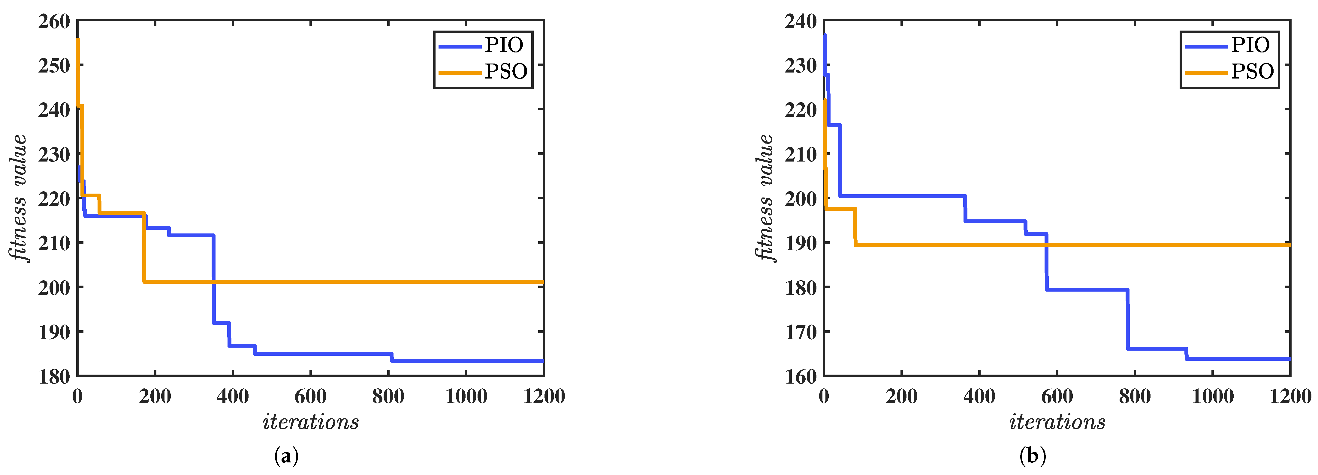The PIO algorithm and the particle swarm optimization (PSO) algorithm are compared by using the same populations and iterations. Figure 10 shows the changes in the fitness value of two algorithms during the optimization process. As shown in Figure 10, despite the PIO algorithm exhibiting a convergence speed that is lower than that of the PSO algorithm, its optimization result possesses a lower fitness value, and the obtained trajectory meets the requirements better.

5.3.1. Optimization Results for Hover-to-Cruise Phase

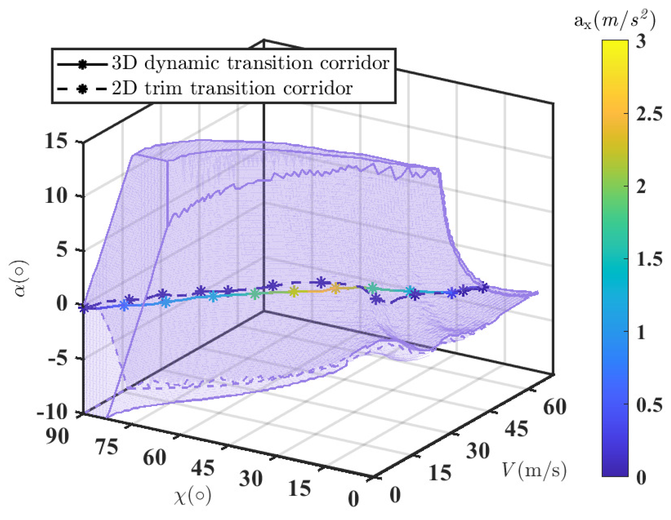
The optimized transition trajectory obtained from the hover-to-cruise dynamic transition corridor is shown in Figure 11. This figure illustrates the change in forward acceleration of the tilt-rotor UAV during the hover-to-cruise phase. For the hover-to-cruise phase, the aircraft acceleration mainly changes when $\chi \in [{10}^{\circ },{70}^{\circ }]$. This is because acceleration can bring the AoA closer to the desired AoA.

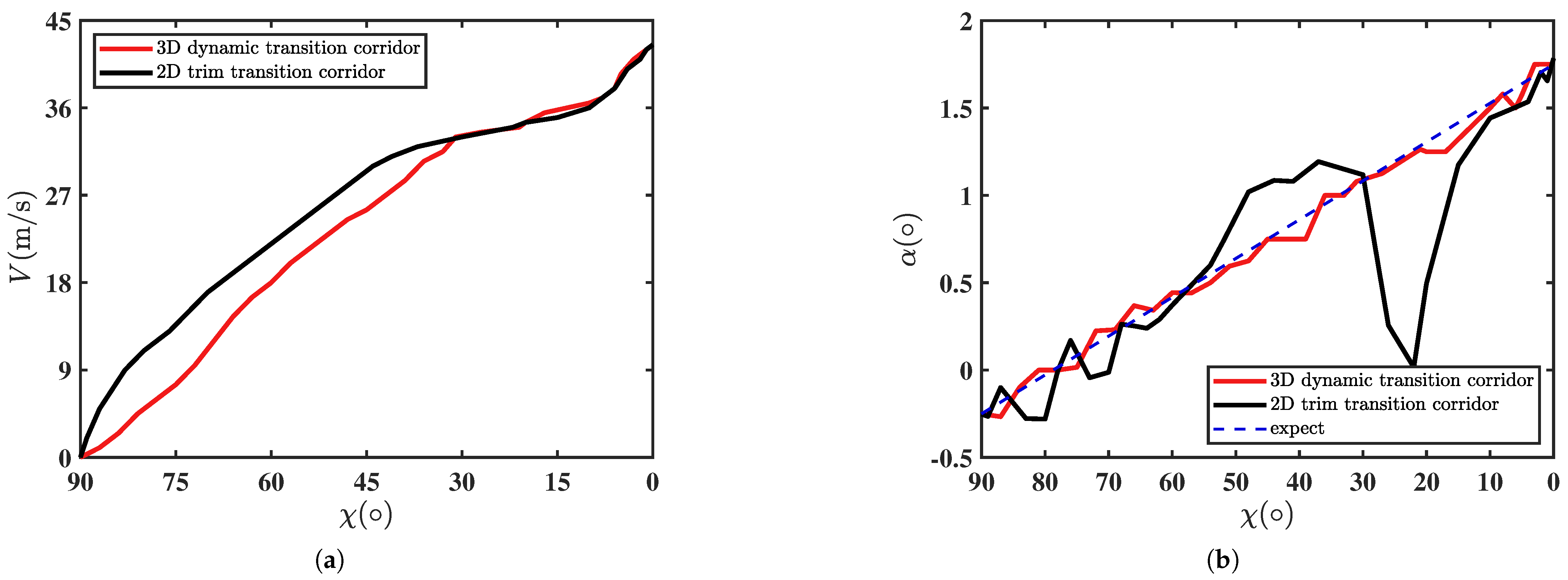
Figure 12 shows the variations in velocity and AoA with respect to the nacelle angle during the hover-to-cruise phase. Compared with the transition trajectory obtained using the two-dimensional trim corridor, the optimized velocity based on the dynamic transition corridor varies smoothly with changes in the nacelle angle, and the gap between the optimized AoA and the desired AoA is relatively small. The AoA curve obtained by the two-dimensional trim transition corridor in Figure 12b is significantly different from the expected AoA in the middle of the transition phase. This is because the aircraft must maintain an increase in its forward speed during the transition phase. Therefore, the AoA of the trim point selected in the trajectory is relatively large.

Figure 13 shows the variations in each control quantity with respect to the velocity during the hover-to-cruise phase of the tilt-rotor UAV. During the transition phase, each actuator has a sufficient control margin. The increase in the main propeller speed after optimization is due to the forward acceleration of the tilt-rotor UAV in the transition phase.

5.3.2. Optimization Results for Cruise-to-Hover Phase

The optimized transition trajectory obtained from the cruise-to-hover dynamic transition corridor is shown in Figure 14. For the cruise-to-hover phase, the acceleration changes in the near-cruise phase. This is because, at the beginning of the transition phase, the aircraft’s AoA is expected to change rapidly and the aircraft will be able to fly at a larger AoA in a decelerated flight state.

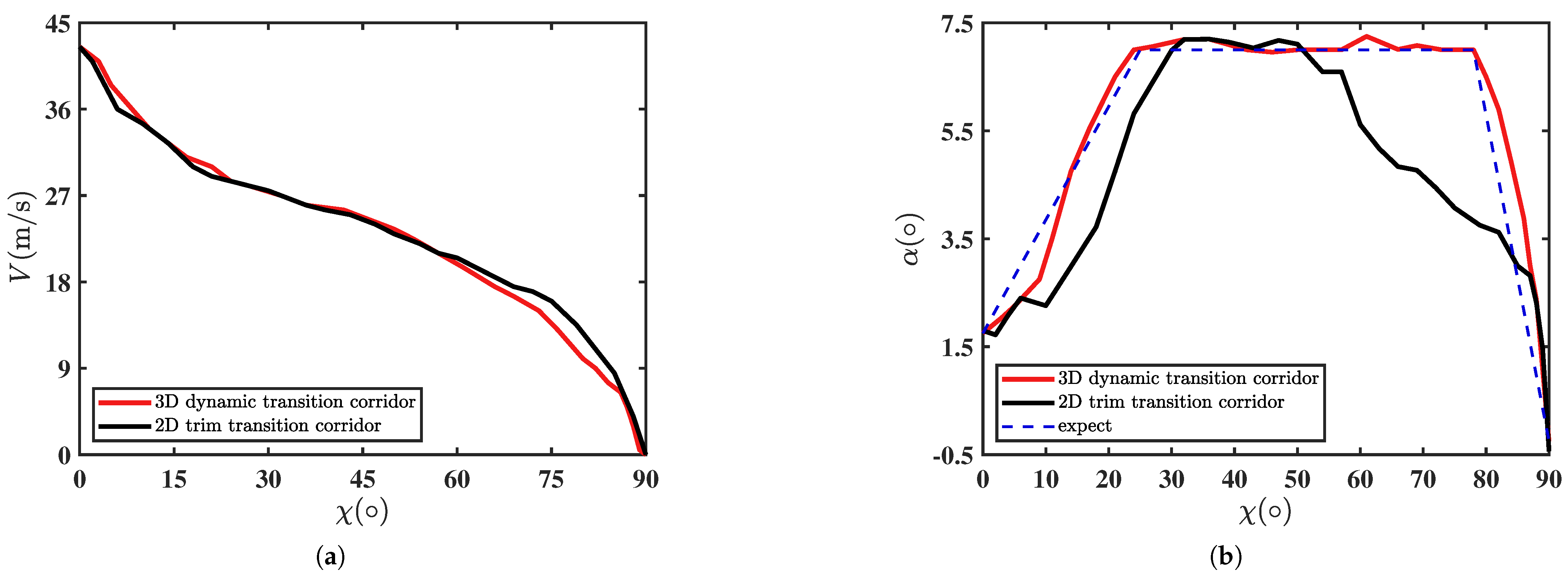
Figure 15 shows the variations in velocity and AoA with respect to the nacelle angle during the cruise-to-hover phase. Compared with the transition trajectory obtained based on the two-dimensional trim corridor, the velocity trajectories optimized based on the dynamic transition corridor vary more smoothly with changes in the nacelle angle. The optimized AoA achieves the desired value faster and the aircraft can fly with a larger AoA in the middle of the transition phase.

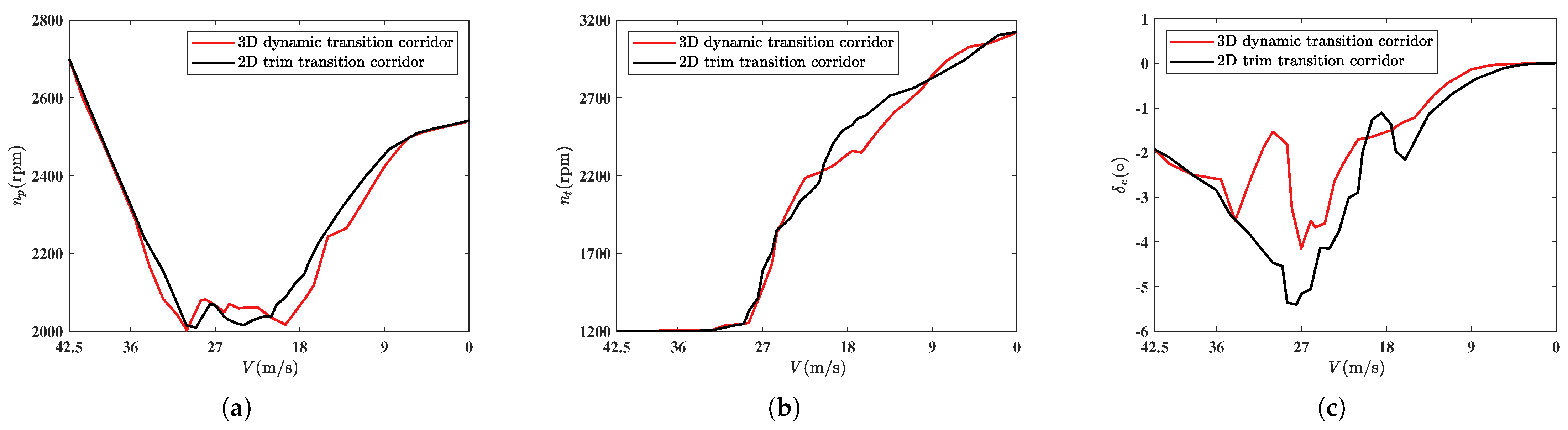
Figure 16 shows the variations in each control quantity during the cruise-to-hover phase of the tilt-rotor UAV. In the cruise-to-hover phase, each actuator has a sufficient control margin. During the pre-transition period, the main propeller speed is reduced due to the aircraft’s deceleration. Late in the transition phase, the optimized main propeller speed is less than the trajectory of the two-dimensional corridor. This is because the aircraft has a large AoA at this stage and the aerodynamic forces generated provide some of the lift.

6. Conclusions

This paper has described research on a characterization method for the transition corridor and an optimization method for the transition trajectory of tilt-rotor UAVs. First, a component modeling method was used to model the tilt-rotor UAV. Based on this, a dynamic transition corridor characterization method considering the dynamic characteristics of acceleration and deceleration during the transition phase was proposed. Based on the established three-dimensional dynamic transition corridor, a transition trajectory optimization method was derived using the PIO algorithm. Numerical simulations have shown that, compared with the transition trajectory obtained based on the two-dimensional transition corridor, the proposed method ensures smoother changes in the velocity, nacelle angle, and expected AoA during the transition phase. The research results provide a solid foundation for the study of transition phase control strategies.

In the future, we first study the trajectory optimization method for the uncertain dynamic model of the tilt-rotor aircraft, including the optimization analysis of the modeling uncertainty of each aircraft component and the uncertainty of the flight environment. Secondly, we will analyze the structural load distributions on key components during the transition phase. In addition, more flight tests for the transition phase will be conducted.

References

1. Silva Castilho, D.; Andrade, D. Is the tiltrotor worthy for civilian transportation between grea cities? ERF 2012. [Google Scholar]
2. Karimli, Y.; Marano, A.D. Exploring the Promises and Challenges of Urban Air Mobility (UAM). Adv. Aerosp. Sci. Technol. 2024, 9, 75–84. [Google Scholar] [CrossRef]
3. Misra, A.; Jayachandran, S.; Kenche, S.; Katoch, A.; Suresh, A.; Gundabattini, E.; Selvaraj, S.K.; Legesse, A.A. A Review on Vertical Take-Off and Landing (VTOL) Tilt-Rotor and Tilt Wing Unmanned Aerial Vehicles (UAVs). J. Eng. 2022, 2022, 1803638. [Google Scholar] [CrossRef]
4. Yan, X.; Lou, B.; Xie, A.; Chen, L.; Zhang, D. A review of advanced high-speed rotorcraf. IOP Conf. Ser. Mater. Sci. Eng. (MSE) 2021, 1102, 012006. [Google Scholar] [CrossRef]
5. Rehan, M.; Akram, F.; Shahzad, A.; Shams, T.A.; Ali, Q. Vertical take-off and landing hybrid unmanned aerial vehicles: An overview. Aeronaut. J. 2022, 126, 2017–2057. [Google Scholar] [CrossRef]
6. Liu, Z.; He, Y.; Yang, L.; Han, J. Control techniques of tilt rotor unmanned aerial vehicle systems: A review. Chin. J. Aeronaut. 2017, 30, 135–148. [Google Scholar] [CrossRef]
7. Yuan, L.; Zhang, W.; Wen, X. Study on Model and Simulation of the Tilt Rotor Aircraft in Transition Mode. In Proceedings of the International Conference on Advances in Mechanical Engineering and Industrial Informatics (AMEII 2015), Shenyang, China, 11–12 April 2015. [Google Scholar]
8. Bhardwaj, P.; Raab, S.A.; Zhang, J.; Holzapfel, F. Integrated reference model for a tilt-rotor vertical take-off and landing transition uav. In Proceedings of the 2018 Applied Aerodynamics Conference, Atlanta, GA, USA, 25–29 June 2018. [Google Scholar]
9. Chen, S.; Yang, Y.; Zhang, X.; Wang, B. Research on transition corridor of distributed tilting power configuration. J. Phys. Conf. Ser. 2024, 2691, 012029. [Google Scholar] [CrossRef]
10. Song, W.; Sun, L.; Wang, Q. Nonlinear Constrained Optimization Method for Dynamic Conversion Corridor of Tilt-Rotor Aircraft. J. Guid. Control Dynam. 2024, 47, 2661–2666. [Google Scholar] [CrossRef]
11. Zhang, S.; Yang, Y.; Wang, X.; Zhu, J.; Zhang, X. Modeling and dynamic analysis of a distributed propulsion tilt-rotor aircraft. In Proceedings of the AIAA Aviation 2022 Forum, Chicago, IL, USA, 27 June–1 July 2022. [Google Scholar]
12. Yu, X. Flight Dynamies Modeling and Control Methods of Tiltrotor Aircraft Coupled with Dynamic Tilting Characteristics of Rotor. Doctoral Dissertation, Nanjing University of Aeronautics and Astronautics, Nanjing, China, 2023. [Google Scholar]
13. May, M.S.; Milz, D.; Looye, G. Towards the Determination of the Dynamic Transition Corridor for Tandem Tilt-Wing Aircraft. In Proceedings of the AIAA Aviation Forum and Ascend 2024, Las Vegas, NV, USA, 29 July–2 August 2024. [Google Scholar]
14. Cheng, Z.; Pei, H. A corridor-based flight mode transition strategy for agile ducted-fan tail-sitter UAV:Altitude-hold transition. Chin. J. Aeronaut. 2023, 36, 330–345. [Google Scholar] [CrossRef]
15. Xiao, J. Design of Flight Control Law for the New Configuration Unmanned Tilt-Rotor Aircraftin Transition State. Doctoral Dissertation, Nanjing University of Aeronautics and Astronautics, Nanjing, China, 2021. [Google Scholar]
16. Zuo, Z.; Ye, Z.Q.; Xiao, S.Q.; Huang, Y. Research on Conversion Trajectory Design of Tilt-rotor UAV. EEA 2021, 50, 167–172. [Google Scholar]
17. Hyun, J.; Jang, M.; Nguyen, T.A.; Lee, J.-W. Transition control planning and optimization for a boxed-wing eVTOL tiltrotor vehicle using trim analysis. In Proceedings of the 2023 International Conference on Unmanned Aircraft Systems (ICUAS), Warsaw, Poland, 6–9 June 2023. [Google Scholar]
18. Zhang, Z.; Tian, J.; Chen, H.; Sheng, S. Optimal Transition Trajectory Search for Tilt-Rotor Aircraft Based on Ant Colony Algorithm. In Proceedings of the 2023 2nd International Conference on Artificial Intelligence and Computer Information Technology (AICIT), Yichang, China, 15–17 September 2023. [Google Scholar]
19. Lyu, Z.; Wang, Z.; Duan, D.; Lin, L.; Li, J.; Yang, Y. Tilting path optimization of tilt quad rotor in conversion process based on ant colony optimization algorithm. IEEE Access 2020, 8, 140777–140791. [Google Scholar] [CrossRef]
20. Zhou, X.Q.; Xu, J.F. Analysis of 3D conversion corridor and establishment of transition path for tilting quadcopter aircraft. AASE 2024. [Google Scholar]
21. Chen, Z.; Zhang, Z.; Sheng, S.; Yuan, S. Transition Trajectory Planning for Tilt-Rotor Aircraft Based on SA-IGA Algorithm. In Proceedings of the 2024 International Conference on Guidance, Navigation and Control (ICGNC), Changsha, China, 9–11 August 2024. [Google Scholar]
22. Duan, H.; Qiao, P. Pigeon-inspired optimization: A new swarm intelligence optimizer for air robot path planning. Int. J. Intell. Comput. Cybern. 2014, 7, 24–37. [Google Scholar] [CrossRef]
Figure 1. Layout of the tilt-rotor UAV.
Drones 09 00432 g001
Figure 2. Lift coefficient of the tilt-rotor aircraft wing.
Drones 09 00432 g002
Figure 3. Two-dimensional trim transition corridor.
Drones 09 00432 g003
Figure 4. Two-dimensional trim transition corridor taking into account model uncertainty. (a) Uncertainty of main propeller thrust coefficient. (b) Uncertainty of wing lift coefficient.
Drones 09 00432 g004
Figure 5. Three-dimensional trim transition corridor: (a) 3D view; (b) top view.
Drones 09 00432 g005
Figure 6. Dynamic transition corridor for hover-to-cruise phase: (a) 3D view; (b) top view.
Drones 09 00432 g006
Figure 7. Constraints of the dynamic transition corridor for hover-to-cruise phase.
Drones 09 00432 g007
Figure 8. Dynamic transition corridor for hover-to-cruise phase: (a) 3D view; (b) top view.
Drones 09 00432 g008
Figure 9. Constraints of the dynamic transition corridor for cruise-to-hover phase.
Drones 09 00432 g009
Figure 10. Convergence results of fitness values: (a) hover to cruise; (b) cruise to hover.
Drones 09 00432 g010
Figure 11. Optimized transition trajectory given by the PIO algorithm for hover-to-cruise phase.
Drones 09 00432 g011
Figure 12. Variations in velocity and AoA with nacelle angle for hover-to-cruise phase: (a) velocity; (b) AoA.
Drones 09 00432 g012
Figure 13. Variations in control parameters with velocity for hover-to-cruise phase. (a) Main propeller speed. (b) Tail propeller speed. (c) Elevator deflection.
Drones 09 00432 g013
Figure 14. Optimized transition trajectory given by PIO algorithm for cruise-to-hover phase.
Drones 09 00432 g014
Figure 15. Optimized transition trajectory given by PIO algorithm for hover-to-cruise phase. (a) Velocity. (b) AoA.
Drones 09 00432 g015
Figure 16. Variations in control parameters with velocity for cruise-to-hover phase. (a) Main propeller speed. (b) Tail propeller speed. (c) Elevator deflection.
Drones 09 00432 g016