
A Cross-Mamba Interaction Network for UAV-to-Satallite Geolocalization


Abstract
1. Introduction
- (1)
- We propose a simple and effective baseline pipeline, named CMIN, for UAV geolocalization. To the best of our knowledge, this is the first work to utilize a state-space model to capture the global correlation between UAV and satellite from a larger receptive field.
- (2)
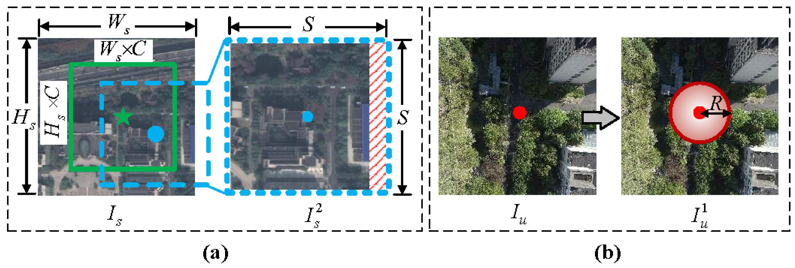
- We present an SFEM to extract shared features from both UAV and satellite images and employ an LCAM to fuse the cross-Mamba features. Moreover, a CM method is introduced for data augmentation, enabling the model to capture more detailed contextual clues.
- (3)
- Extensive experiments show that our method achieves state-of-the-art performance on the benchmark dataset. Specifically, our CMIN achieves 77.52% w.r.t. Relative Distance Score (RDS) metric on the UL14 dataset, outperforming a well-established method [17] by 12.19%. Ablation studies further demonstrate the effectiveness of CMIN for UAV localization.
2. Related Work
2.1. Cross-View Geolocalization
2.2. Mamba in Computer Vision
3. Method
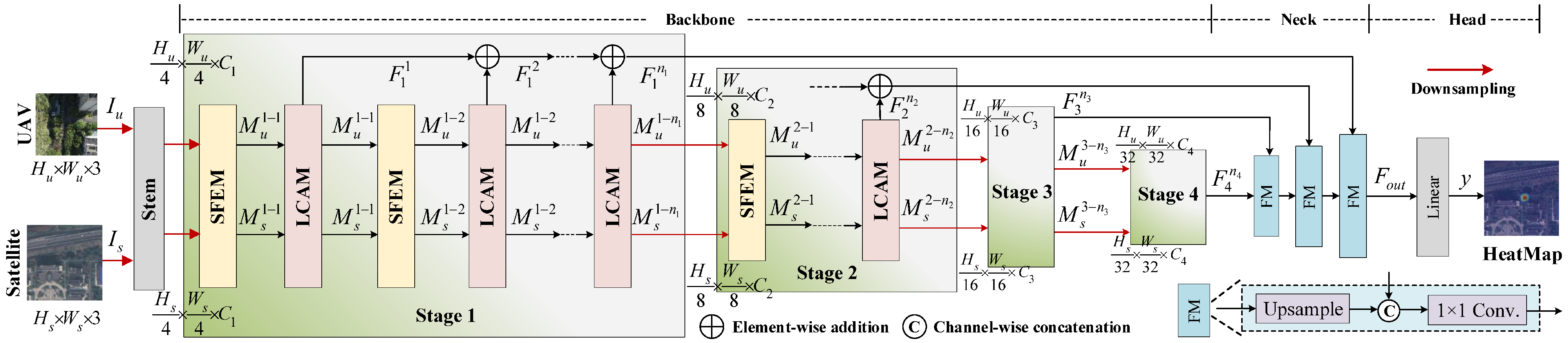
3.1. Overview
3.2. Siamese Feature Extraction Module
3.3. Local Cross-Attention Module
3.4. Training Details
4. Experiment
4.1. Experimental Settings
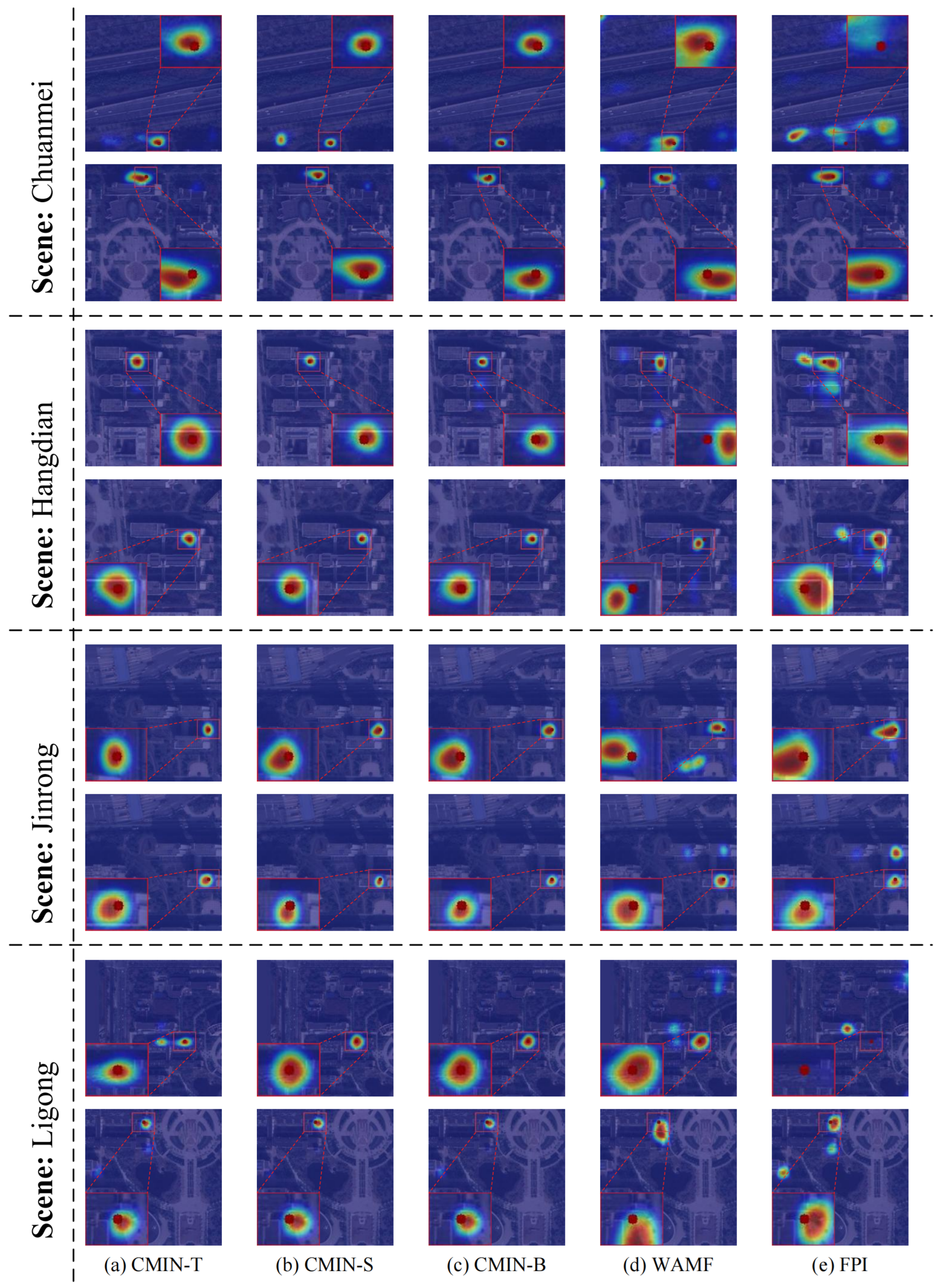
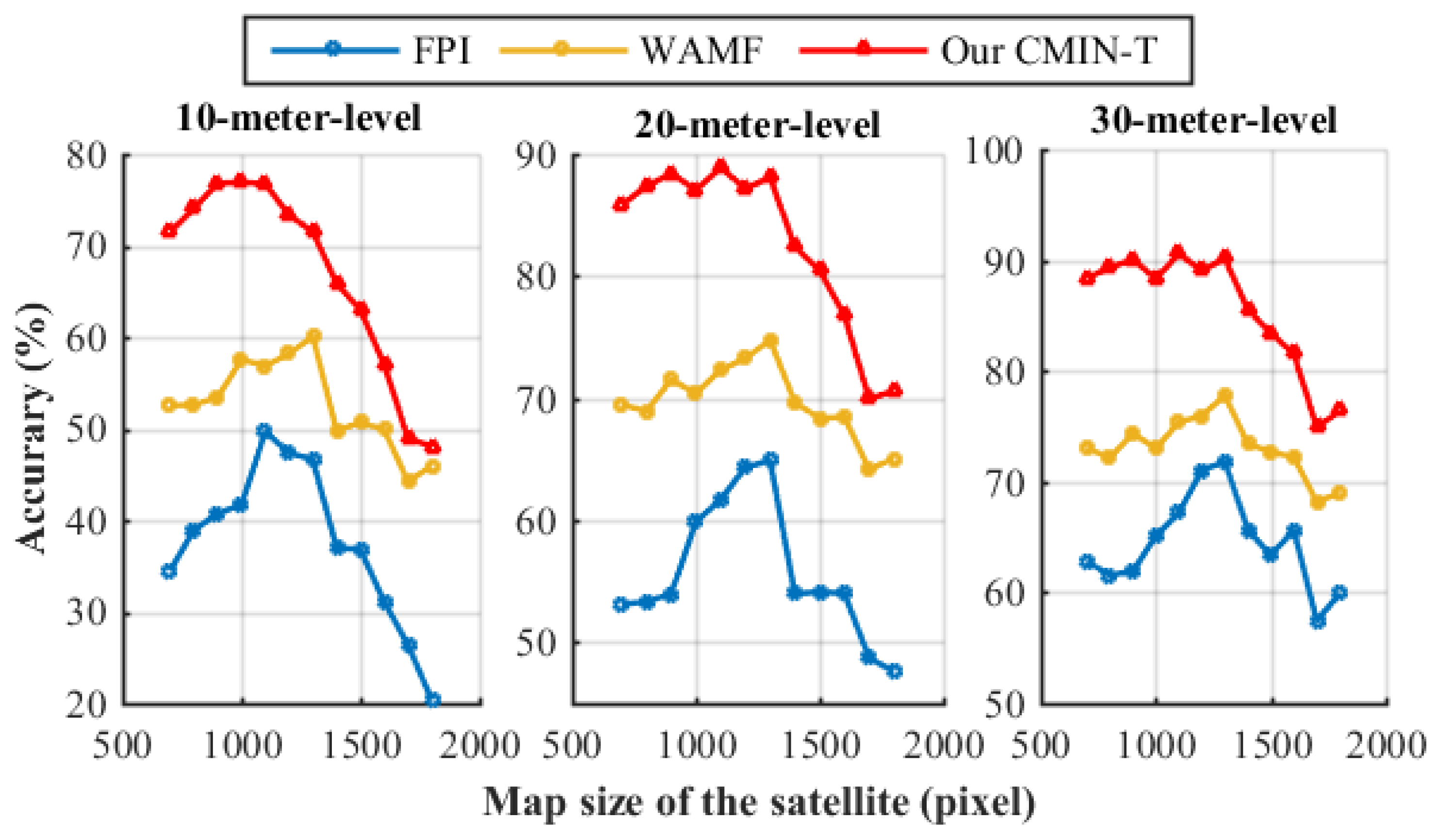
4.2. Comparison with the State-of-the-Art Methods
4.3. Ablation Study
5. Conclusions
Author Contributions
Funding
Data Availability Statement
Conflicts of Interest
References
- Ibraiwish, H.; Eltokhey, M.W.; Alouini, M. UAV-Assisted VLC Using LED-Based Grow Lights in Precision Agriculture Systems. IEEE Internet Things Mag. 2024, 7, 100–105. [Google Scholar] [CrossRef]
- Hu, Z.; Fan, S.; Li, Y.; Tang, Q.; Bao, L.; Zhang, S.; Sarsen, G.; Guo, R.; Wang, L.; Zhang, N.; et al. Estimating Stratified Biomass in Cotton Fields Using UAV Multispectral Remote Sensing and Machine Learning. Drones 2025, 9, 186. [Google Scholar] [CrossRef]
- Huang, D.; Wang, Y.; Li, H. Study on UAV Inspection Safety Distance of Substation High-Voltage and Current-Carrying Equipment Based on Power-Frequency Magnetic Field. IEEE Trans. Instrum. Meas. 2024, 73, 3539008. [Google Scholar] [CrossRef]
- Xu, J.; Fan, X.; Jian, H.; Xu, C.; Bei, W.; Ge, Q.; Zhao, T. YoloOW: A Spatial Scale Adaptive Real-Time Object Detection Neural Network for Open Water Search and Rescue From UAV Aerial Imagery. IEEE Trans. Geosci. Remote Sens. 2024, 62, 5623115. [Google Scholar] [CrossRef]
- Gaigalas, J.; Perkauskas, L.; Gricius, H.; Kanapickas, T.; Kriščiūnas, A. A Framework for Autonomous UAV Navigation Based on Monocular Depth Estimation. Drones 2025, 9, 236. [Google Scholar] [CrossRef]
- Kramarić, L.; Jelušić, N.; Radišić, T.; Muštra, M. A Comprehensive Survey on Short-Distance Localization of UAVs. Drones 2025, 9, 188. [Google Scholar] [CrossRef]
- Lin, J.; Zheng, Z.; Zhong, Z.; Luo, Z.; Li, S.; Yang, Y.; Sebe, N. Joint Representation Learning and Keypoint Detection for Cross-View Geo-Localization. IEEE Trans. Image Process. 2022, 31, 3780–3792. [Google Scholar] [CrossRef]
- Liang, Y.; Wu, X. Do Keypoints Contain Crucial Information? Mining Keypoint Information to Enhance Cross-View Geo-Localization. In Proceedings of the IEEE International Conference on Multimedia and Expo (ICME), Niagara Falls, ON, Canada, 15–19 July 2024; pp. 1–6. [Google Scholar]
- Li, Q.; Yang, X.; Fan, J.; Lu, R.; Tang, B.; Wang, S.; Su, S. GeoFormer: An Effective Transformer-Based Siamese Network for UAV Geolocalization. IEEE J. Sel. Top. Appl. Earth Obs. Remote Sens. 2024, 17, 9470–9491. [Google Scholar] [CrossRef]
- Bellavia, F. SIFT Matching by Context Exposed. IEEE Trans. Pattern Anal. Mach. Intell. 2023, 45, 2445–2457. [Google Scholar] [CrossRef]
- Ding, L.; Zhou, J.; Meng, L.; Long, Z. A Practical Cross-View Image Matching Method between UAV and Satellite for UAV-Based Geo-Localization. Remote Sens. 2021, 13, 47. [Google Scholar] [CrossRef]
- Gong, N.; Li, L.; Sha, J.; Sun, X.; Huang, Q. A Satellite-Drone Image Cross-View Geolocalization Method Based on Multi-Scale Information and Dual-Channel Attention Mechanism. Remote Sens. 2024, 16, 941. [Google Scholar] [CrossRef]
- Tian, X.; Shao, J.; Ouyang, D.; Shen, H.T. UAV-Satellite View Synthesis for Cross-View Geo-Localization. IEEE Trans. Circuits Syst. Video Technol. 2022, 32, 4804–4815. [Google Scholar] [CrossRef]
- Dai, M.; Hu, J.; Zhuang, J.; Zheng, E. A Transformer-Based Feature Segmentation and Region Alignment Method for UAV-View Geo-Localization. IEEE Trans. Circuits Syst. Video Technol. 2022, 32, 4376–4389. [Google Scholar] [CrossRef]
- Wang, Z.; Shi, D.; Qiu, C.; Jin, S.; Li, T.; Shi, Y.; Liu, Z.; Qiao, Z. Sequence Matching for Image-Based UAV-to-Satellite Geolocalization. IEEE Trans. Geosci. Remote Sens. 2024, 62, 5607815. [Google Scholar] [CrossRef]
- Dai, M.; Chen, J.; Lu, Y.; Hao, W.; Zheng, E. Finding Point with Image: An End-to-End Benchmark for Vision-based UAV Localization. arXiv 2022, arXiv:2208.06561. [Google Scholar]
- Wang, G.; Chen, J.; Dai, M.; Zheng, E. WAMF-FPI: A Weight-Adaptive Multi-Feature Fusion Network for UAV Localization. Remote Sens. 2023, 15, 910. [Google Scholar] [CrossRef]
- Chen, J.; Zheng, E.; Dai, M.; Chen, Y.; Lu, Y. OS-FPI: A Coarse-to-Fine One-Stream Network for UAV Geolocalization. IEEE J. Sel. Top. Appl. Earth Obs. Remote Sens. 2024, 17, 7852–7866. [Google Scholar] [CrossRef]
- Liu, Y.; Tian, Y.; Zhao, Y.; Yu, H.; Xie, L.; Wang, Y.; Ye, Q.; Liu, Y. VMamba: Visual State Space Model. arXiv 2024, arXiv:2401.10166. [Google Scholar]
- Zou, Z.; Yu, H.; Huang, J.; Zhao, F. FreqMamba: Viewing Mamba from a Frequency Perspective for Image Deraining. In Proceedings of the MM’24: The 32nd ACM International Conference on Multimedia, Melbourne, VIC, Australia, 28 October–1 November 2024; pp. 1905–1914. [Google Scholar]
- Guo, H.; Li, J.; Dai, T.; Ouyang, Z.; Ren, X.; Xia, S. MambaIR: A Simple Baseline for Image Restoration with State-Space Model. In Proceedings of the ECCV, Milan, Italy, 29 September–4 October 2024; pp. 222–241. [Google Scholar]
- Zamir, A.R.; Shah, M. Image Geo-Localization Based on MultipleNearest Neighbor Feature Matching UsingGeneralized Graphs. IEEE Trans. Pattern Anal. Mach. Intell. 2014, 36, 1546–1558. [Google Scholar] [CrossRef]
- Kim, H.J.; Dunn, E.; Frahm, J. Learned Contextual Feature Reweighting for Image Geo-Localization. In Proceedings of the CVPR, Honolulu, HI, USA, 21–26 July 2017; pp. 3251–3260. [Google Scholar]
- Cai, S.; Guo, Y.; Khan, S.H.; Hu, J.; Wen, G. Ground-to-Aerial Image Geo-Localization With a Hard Exemplar Reweighting Triplet Loss. In Proceedings of the ICCV, Seoul, Republic of Korea, 27 October–2 November 2019; pp. 8390–8399. [Google Scholar]
- Zeng, Z.; Wang, Z.; Yang, F.; Satoh, S. Geo-Localization via Ground-to-Satellite Cross-View Image Retrieval. IEEE Trans. Multim. 2023, 25, 2176–2188. [Google Scholar] [CrossRef]
- Shi, Y.; Liu, L.; Yu, X.; Li, H. Spatial-Aware Feature Aggregation for Image based Cross-View Geo-Localization. In Proceedings of the NeurIPS, Vancouver, BC, Canada, 8–14 December 2019; pp. 10090–10100. [Google Scholar]
- Zhu, Y.; Sun, B.; Lu, X.; Jia, S. Geographic Semantic Network for Cross-View Image Geo-Localization. IEEE Trans. Geosci. Remote Sens. 2022, 60, 4704315. [Google Scholar] [CrossRef]
- Zhu, S.; Shah, M.; Chen, C. TransGeo: Transformer Is All You Need for Cross-view Image Geo-localization. In Proceedings of the CVPR, New Orleans, LA, USA, 18–24 June 2022; pp. 1152–1161. [Google Scholar]
- Gu, A.; Johnson, I.; Goel, K.; Saab, K.; Dao, T.; Rudra, A.; Ré, C. Combining Recurrent, Convolutional, and Continuous-time Models with Linear State Space Layers. In Proceedings of the NeurIPS, Virtual, 6–14 December 2021; pp. 572–585. [Google Scholar]
- Smith, J.T.H.; Warrington, A.; Linderman, S.W. Simplified State Space Layers for Sequence Modeling. In Proceedings of the ICLR, Kigali, Rwanda, 1–5 May 2023. [Google Scholar]
- Ma, X.; Zhou, C.; Kong, X.; He, J.; Gui, L.; Neubig, G.; May, J.; Zettlemoyer, L. Mega: Moving Average Equipped Gated Attention. In Proceedings of the ICLR, Kigali, Rwanda, 1–5 May 2023. [Google Scholar]
- Fu, D.Y.; Epstein, E.L.; Nguyen, E.; Thomas, A.W.; Zhang, M.; Dao, T.; Rudra, A.; Ré, C. Simple Hardware-Efficient Long Convolutions for Sequence Modeling. In Proceedings of the ICML, Kigali, Rwanda, 1–5 May 2023; pp. 10373–10391. [Google Scholar]
- Li, Y.; Cai, T.; Zhang, Y.; Chen, D.; Dey, D. What Makes Convolutional Models Great on Long Sequence Modeling? In Proceedings of the ICLR, Kigali, Rwanda, 1–5 May 2023. [Google Scholar]
- Gu, A.; Dao, T. Mamba: Linear-Time Sequence Modeling with Selective State Spaces. arXiv 2023, arXiv:2312.00752. [Google Scholar]
- He, Y.; Tu, B.; Jiang, P.; Liu, B.; Li, J.; Plaza, A. IGroupSS-Mamba: Interval Group Spatial-Spectral Mamba for Hyperspectral Image Classification. IEEE Trans. Geosci. Remote Sens. 2024, 62, 5538817. [Google Scholar] [CrossRef]
- Yang, A.; Li, M.; Ding, Y.; Fang, L.; Cai, Y.; He, Y. GraphMamba: An Efficient Graph Structure Learning Vision Mamba for Hyperspectral Image Classification. IEEE Trans. Geosci. Remote Sens. 2024, 62, 5537414. [Google Scholar] [CrossRef]
- Ding, H.; Xia, B.; Liu, W.; Zhang, Z.; Zhang, J.; Wang, X.; Xu, S. A Novel Mamba Architecture with a Semantic Transformer for Efficient Real-Time Remote Sensing Semantic Segmentation. Remote Sens. 2024, 16, 2620. [Google Scholar] [CrossRef]
- Yang, Y.; Ma, C.; Yao, J.; Zhong, Z.; Zhang, Y.; Wang, Y. ReMamber: Referring Image Segmentation with Mamba Twister. In Proceedings of the ECCV, MiCo Milano, Italy, 29 September–4 October 2024; pp. 108–126. [Google Scholar]
- Howard, A.G.; Zhu, M.; Chen, B.; Kalenichenko, D.; Wang, W.; Weyand, T.; Andreetto, M.; Adam, H. MobileNets: Efficient Convolutional Neural Networks for Mobile Vision Applications. arXiv 2017, arXiv:1704.04861. [Google Scholar]
- Zhao, Y.; Luo, C.; Zha, Z.; Zeng, W. Multi-Scale Group Transformer for Long Sequence Modeling in Speech Separation. In Proceedings of the IJCAI, Yokohama, Japan, 11–17 July 2020; pp. 3251–3257. [Google Scholar]
- Li, Z.; Liu, X.; Drenkow, N.; Ding, A.S.; Creighton, F.X.; Taylor, R.H.; Unberath, M. Revisiting Stereo Depth Estimation From a Sequence-to-Sequence Perspective with Transformers. In Proceedings of the ICCV, Virtual, 11–17 October 2021; pp. 6177–6186. [Google Scholar]
- Xu, W.; Yao, Y.; Cao, J.; Wei, Z.; Liu, C.; Wang, J.; Peng, M. UAV-VisLoc: A Large-scale Dataset for UAV Visual Localization. arXiv 2024, arXiv:2405.11936. [Google Scholar]
- Deng, J.; Dong, W.; Socher, R.; Li, L.; Li, K.; Fei-Fei, L. ImageNet: A large-scale hierarchical image database. In Proceedings of the CVPR, Miami, FL, USA, 20–25 June 2009; pp. 248–255. [Google Scholar]
- Loshchilov, I.; Hutter, F. Decoupled Weight Decay Regularization. In Proceedings of the ICLR, New Orleans, LA, USA, 6–9 May 2019. [Google Scholar]
- Wang, T.; Zheng, Z.; Yan, C.; Zhang, J.; Sun, Y.; Zheng, B.; Yang, Y. Each Part Matters: Local Patterns Facilitate Cross-View Geo-Localization. IEEE Trans. Circuits Syst. Video Technol. 2022, 32, 867–879. [Google Scholar] [CrossRef]
- Shen, T.; Wei, Y.; Kang, L.; Wan, S.; Yang, Y. MCCG: A ConvNeXt-Based Multiple-Classifier Method for Cross-View Geo-Localization. IEEE Trans. Circuits Syst. Video Technol. 2024, 34, 1456–1468. [Google Scholar] [CrossRef]
- He, K.; Zhang, X.; Ren, S.; Sun, J. Deep Residual Learning for Image Recognition. In Proceedings of the 2016 IEEE Conference on Computer Vision and Pattern Recognition, CVPR 2016, Las Vegas, NV, USA, 27–30 June 2016; IEEE Computer Society: Washington, DC, USA, 2016; pp. 770–778. [Google Scholar] [CrossRef]
- Dosovitskiy, A.; Beyer, L.; Kolesnikov, A.; Weissenborn, D.; Zhai, X.; Unterthiner, T.; Dehghani, M.; Minderer, M.; Heigold, G.; Gelly, S.; et al. An Image is Worth 16x16 Words: Transformers for Image Recognition at Scale. In Proceedings of the 9th International Conference on Learning Representations, ICLR 2021, Virtual Event, Austria, 3–7 May 2021; OpenReview.net: Alameda, CA, USA, 2021. [Google Scholar]
- Huang, T.; Pei, X.; You, S.; Wang, F.; Qian, C.; Xu, C. LocalMamba: Visual State Space Model with Windowed Selective Scan. arXiv 2024, arXiv:2403.09338. [Google Scholar]


| Method | RDS | MA@3 | MA@10 | MA@20 | |
|---|---|---|---|---|---|
| Image retrieval | LCM [11] | - | 0.014 | 0.112 | 0.250 |
| LPN [45] | - | 0.015 | 0.158 | 0.273 | |
| RKNet [7] | - | 0.021 | 0.177 | 0.317 | |
| MCCG [46] | - | 0.078 | 0.574 | 0.752 | |
| FSRA [14] | - | 0.079 | 0.580 | 0.743 | |
| Heatmap regression | FPI [16] | 57.22% | - | 0.384 | 0.577 |
| WAMF [17] | 65.33% | 0.125 | 0.526 | 0.697 | |
| OS-FPI* [18] | 66.22% | 0.157 | 0.576 | 0.706 | |
| OS-FPI [18] | 76.25% | 0.228 | 0.723 | 0.825 | |
| Our CMIN-T | 75.23% | 0.177 | 0.661 | 0.818 | |
| Our CMIN-S | 76.74% | 0.199 | 0.701 | 0.837 | |
| Our CMIN-B | 77.52% | 0.204 | 0.713 | 0.850 | |
| Method | RDS | MA@3 | MA@10 | MA@20 |
|---|---|---|---|---|
| LPN [45] | - | 0.0009 | 0.0116 | 0.0318 |
| FSRA [14] | - | 0.0011 | 0.0135 | 0.0358 |
| FPI [16] | 15.82% | 0.0012 | 0.0152 | 0.0447 |
| WAMF [17] | 16.23% | 0.0011 | 0.0157 | 0.0464 |
| OS-FPI* [18] | 17.14% | 0.0019 | 0.0194 | 0.0457 |
| OS-FPI [18] | 18.21% | 0.0025 | 0.0230 | 0.0829 |
| Our CMIN-T | 20.01% | 0.0072 | 0.0548 | 0.0938 |
| Our CMIN-S | 31.09% | 0.0860 | 0.2234 | 0.2652 |
| Our CMIN-B | 35.45% | 0.0921 | 0.2280 | 0.3053 |
| Method | GFLOPs | Speed | Parameters | RDS | MA@5 | MA@30 |
|---|---|---|---|---|---|---|
| CMIN-T | 20.9 G | 95.48 FPS | 34.8 M | 75.23% | 0.352 | 0.847 |
| CMIN-S | 34.5 G | 49.24 FPS | 50.2 M | 76.74% | 0.388 | 0.860 |
| CMIN-B | 57.8 G | 40.59 FPS | 88.5 M | 77.52% | 0.396 | 0.872 |
| Method | RDS | MA@3 | MA@5 | MA@20 | MA@30 |
|---|---|---|---|---|---|
| (a) | 70.07% | 0.117 | 0.258 | 0.796 | 0.798 |
| (b) | 75.23% | 0.177 | 0.352 | 0.818 | 0.847 |
| Method | RDS | MA@3 | MA@10 | MA@20 |
|---|---|---|---|---|
| ResNet [47] | 65.15% | 0.112 | 0.512 | 0.662 |
| ViT-S [48] | 70.42% | 0.155 | 0.605 | 0.754 |
| ViT-B [48] | 72.19% | 0.163 | 0.648 | 0.799 |
| VSS [19] | 75.23% | 0.177 | 0.661 | 0.818 |
| LocalVim [49] | 78.67% | 0.182 | 0.716 | 0.863 |
| R | RDS | MA@3 | MA@5 | MA@10 | MA@20 |
|---|---|---|---|---|---|
| 0% | 72.49% | 0.147 | 0.309 | 0.602 | 0.786 |
| 10% | 74.24% | 0.167 | 0.339 | 0.647 | 0.807 |
| 20% | 75.23% | 0.177 | 0.352 | 0.661 | 0.818 |
| 30% | 74.50% | 0.171 | 0.344 | 0.644 | 0.809 |
| RDS | MA@3 | MA@5 | MA@10 | MA@20 | |
|---|---|---|---|---|---|
| 0.2 | 75.03% | 0.173 | 0.347 | 0.648 | 0.821 |
| 0.3 | 75.23% | 0.177 | 0.352 | 0.661 | 0.818 |
| 0.4 | 74.83% | 0.172 | 0.344 | 0.648 | 0.814 |
| 0.5 | 74.64% | 0.172 | 0.342 | 0.644 | 0.812 |
| 0.6 | 74.24% | 0.166 | 0.329 | 0.632 | 0.808 |
Disclaimer/Publisher’s Note: The statements, opinions and data contained in all publications are solely those of the individual author(s) and contributor(s) and not of MDPI and/or the editor(s). MDPI and/or the editor(s) disclaim responsibility for any injury to people or property resulting from any ideas, methods, instructions or products referred to in the content. |
© 2025 by the authors. Licensee MDPI, Basel, Switzerland. This article is an open access article distributed under the terms and conditions of the Creative Commons Attribution (CC BY) license (https://creativecommons.org/licenses/by/4.0/).
Share and Cite
Tian, L.; Shen, Q.; Gao, Y.; Wang, S.; Liu, Y.; Deng, Z. A Cross-Mamba Interaction Network for UAV-to-Satallite Geolocalization. Drones 2025, 9, 427. https://doi.org/10.3390/drones9060427
Tian L, Shen Q, Gao Y, Wang S, Liu Y, Deng Z. A Cross-Mamba Interaction Network for UAV-to-Satallite Geolocalization. Drones. 2025; 9(6):427. https://doi.org/10.3390/drones9060427
Chicago/Turabian StyleTian, Lingyun, Qiang Shen, Yang Gao, Simiao Wang, Yunan Liu, and Zilong Deng. 2025. "A Cross-Mamba Interaction Network for UAV-to-Satallite Geolocalization" Drones 9, no. 6: 427. https://doi.org/10.3390/drones9060427
APA StyleTian, L., Shen, Q., Gao, Y., Wang, S., Liu, Y., & Deng, Z. (2025). A Cross-Mamba Interaction Network for UAV-to-Satallite Geolocalization. Drones, 9(6), 427. https://doi.org/10.3390/drones9060427