
Passive Positioning and Adjustment Strategy for UAV Swarm Considering Formation Electromagnetic Compatibility


Abstract
1. Introduction
2. Materials and Methods
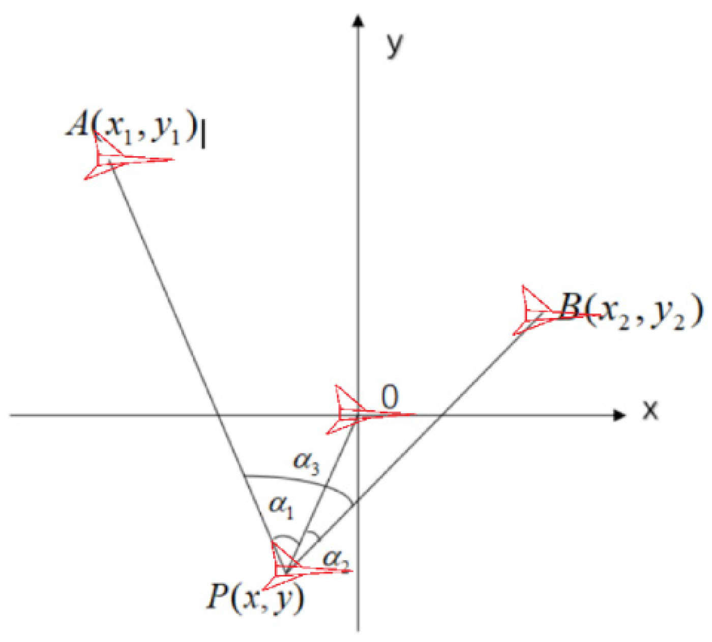
2.1. Determining the Position of the Target Drone Using Vector Methods in a Cartesian Coordinate System
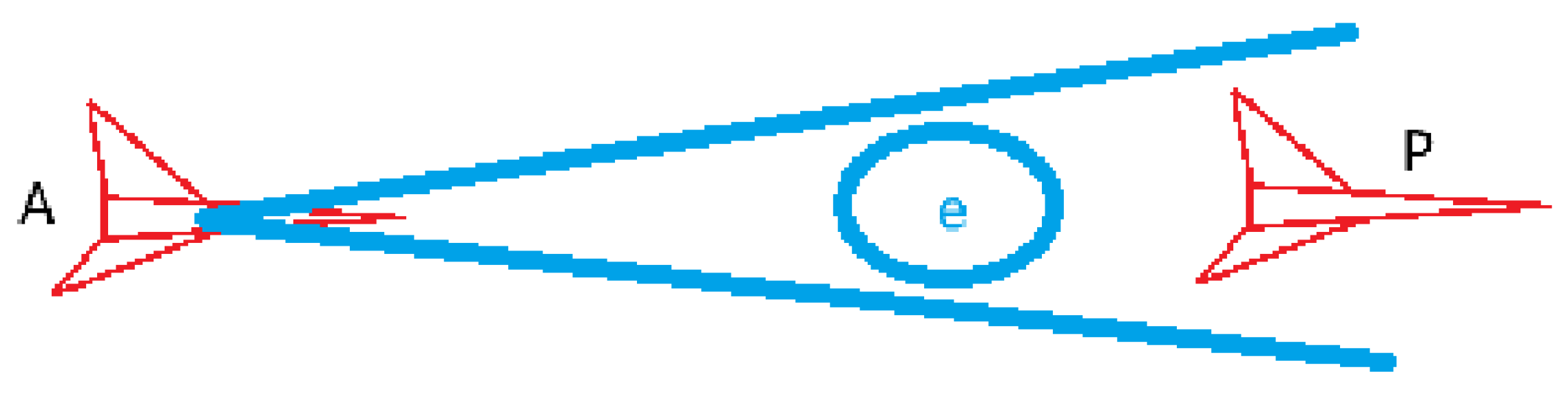
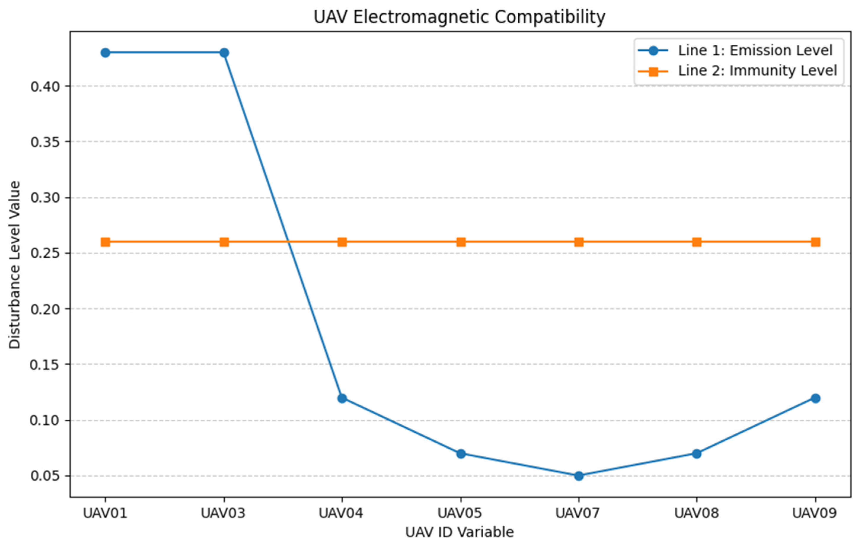
2.2. Analysis of Internal Electromagnetic Interference in UAV Formation Systems
2.3. Establishment of Passive Positioning Model for UAV Formation
2.4. Site Selection Criteria for UAV Formations Under Internal Interference Conditions
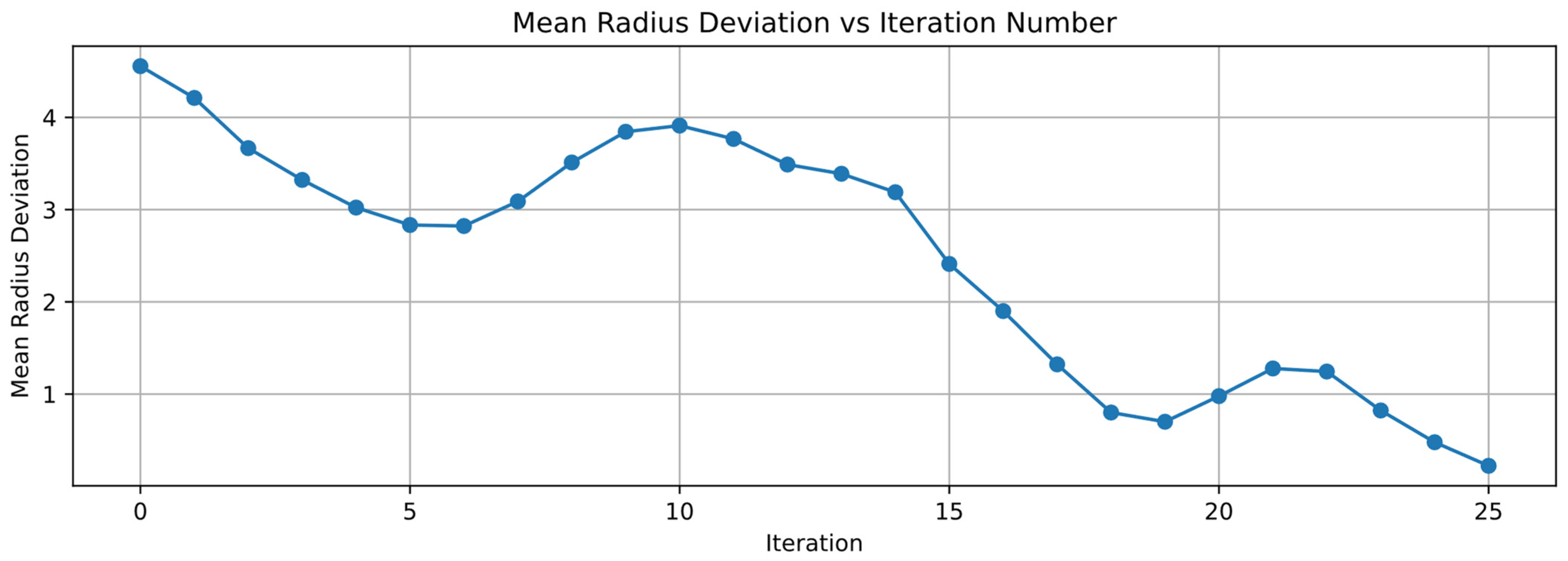
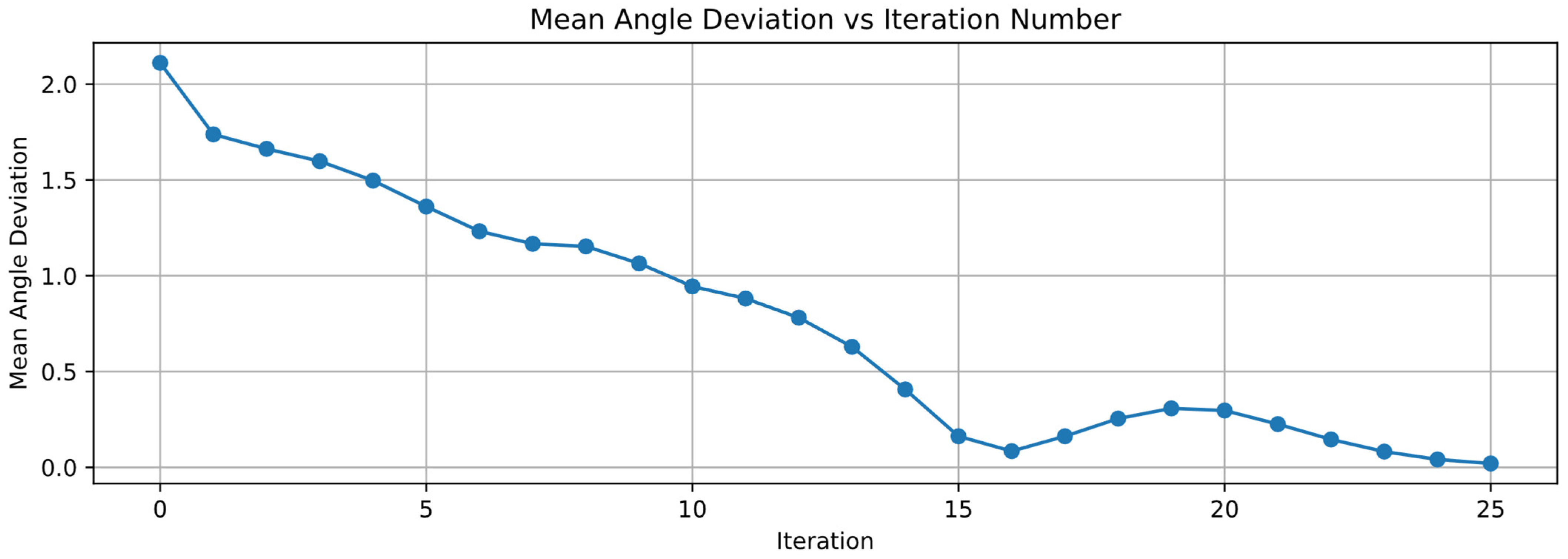
2.5. Passive Positioning Adjustment and Global Iteration
3. Simulation and Results
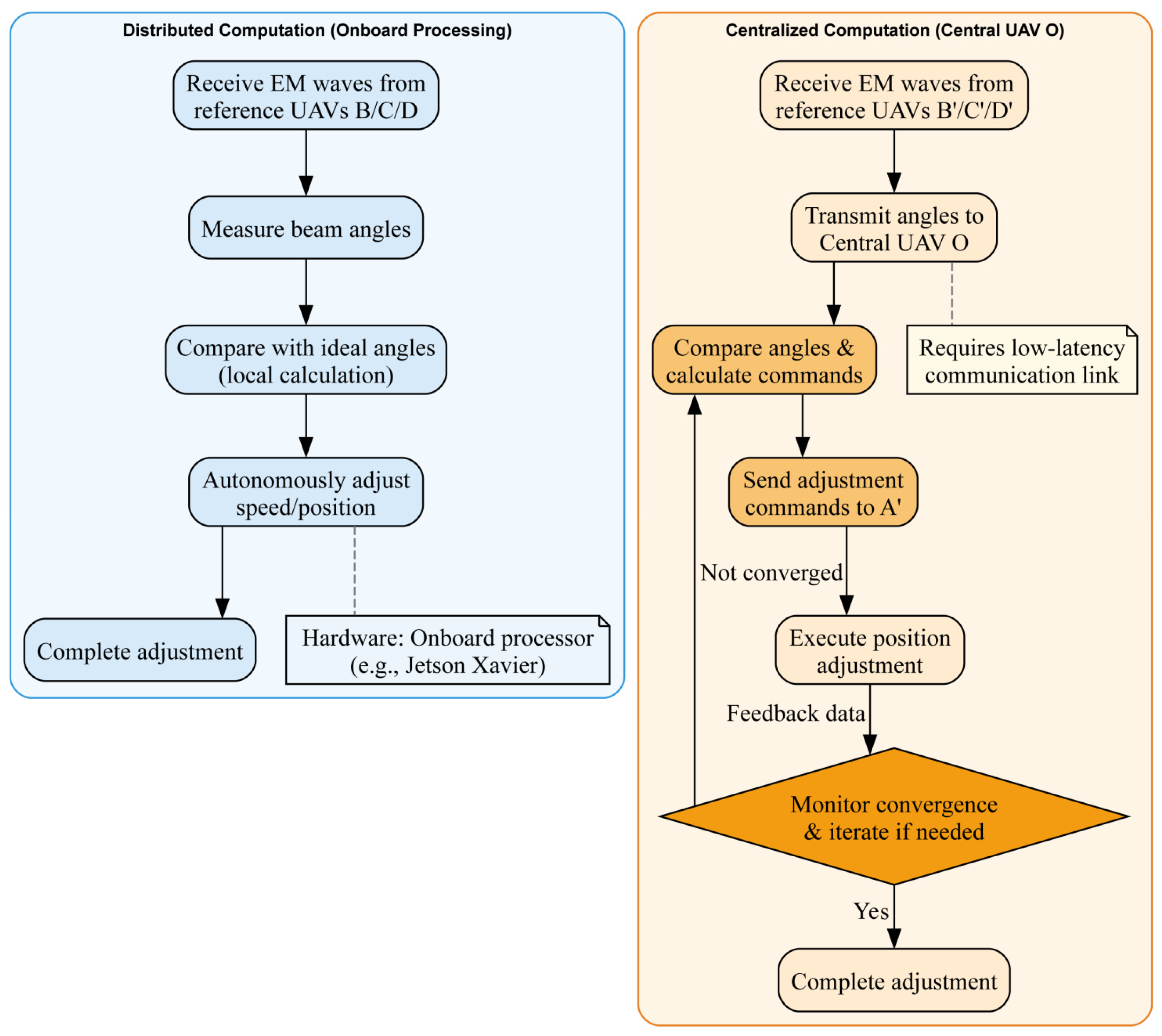
3.1. Signal Transmission Methods and Specific Implementation Processes in Simulation
- A receives electromagnetic waves emitted by three reference drones (B, C, D) and collects the angles between the three beams.
- A compares the current measured angles with the ideal angles at the target position.
- A adjusts its speed to alter its relative position within the formation, bringing the measured angles closer to the ideal angles.
- A completes the positional adjustment.
- A’ receives electromagnetic waves emitted by three reference drones (B’, C’, D’) and collects the angles between the three beams.
- A’ transmits the current measured angles to O.
- O compares the measured angles with the ideal angles at the target position through computation.
- O sends adjustment commands to A’.
- A’ adjusts its speed to alter its relative position and continuously transmits updated angles to O.
- O iteratively issues commands until the measured angles converge to the ideal angles.
- A’ completes the positional adjustment.
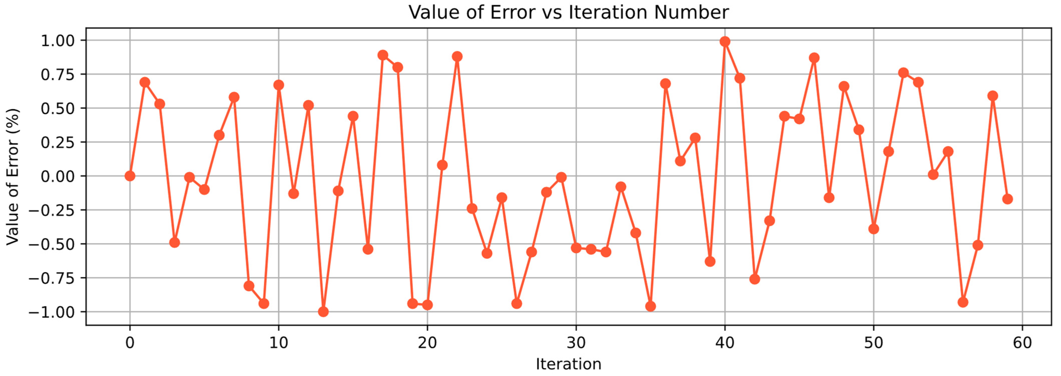
3.2. Simulation Setup and Data Result Analysis
| Algorithm 1. Optimizing UAV Formation Alignment Using Passive Localization Method |
| Input: Initial coordinates of each UAV Termination Condition: #In this simulation, the condition is set as all UAVs must lie within a 1 m radius circle centered at their ideal (unbiased) positions While termination condition is not met: Adjustment for UAV02 UAV02 selects a matching UAV pair for self-localization based on electromagnetic compatibility (EMC) criteria Receives three electromagnetic beams and calculates two angles Compares these angles with the reference angles at the ideal position to compute the proximity scores Adjusts its position to make the received angles closer to the reference angles Reduces the proximity score s ’’’ UAV03 to UAV09 perform similar adjustments ’’’ One iteration completes, and data are collected Check if termination condition is reached |
3.3. Expansion Ideas for Other Formations
4. Discussion of Real-World Deployment
5. Conclusions
Author Contributions
Funding
Data Availability Statement
Acknowledgments
Conflicts of Interest
Appendix A

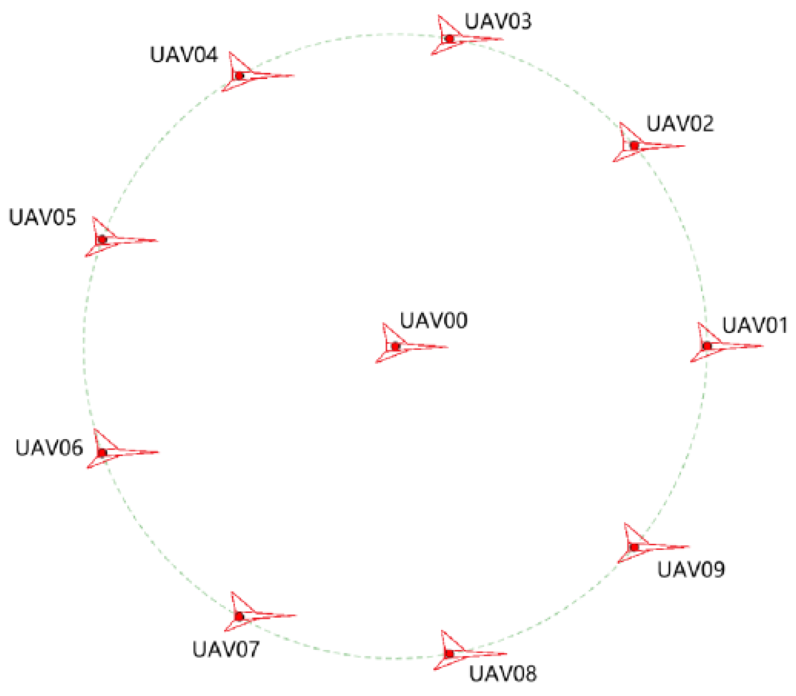
| Drone ID | Standard Position (ρ, θ) | Initial Position (ρ, θ) |
|---|---|---|
| UAV00 | (0, 0) | (0, 0) |
| UAV01 | (100, 0) | (100, 0) |
| UAV02 | (100, 40) | (99, 41) |
| UAV03 | (100, 80) | (102, 80) |
| UAV04 | (−100, 120) | (−105, 119) |
| UAV05 | (−100, 160) | (−97, 159) |
| UAV06 | (−100, 200) | (−108, 195) |
| UAV07 | (−100, 240) | (−105, 240) |
| UAV08 | (−100, 280) | (−98, 280) |
| UAV09 | (−100, 320) | (−112, 321) |
| R1 | UAV01 | UAV03 | UAV04 | UAV05 | UAV06 | UAV07 | UAV08 | UAV09 | |
|---|---|---|---|---|---|---|---|---|---|
| R2 | |||||||||
| UAV01 | / | √ | √ | × | × | × | × | √ | |
| UAV03 | √ | / | √ | × | × | × | × | × | |
| UAV04 | √ | √ | / | √ | √ | √ | √ | √ | |
| UAV05 | × | × | √ | / | √ | √ | √ | √ | |
| UAV06 | × | × | √ | √ | / | √ | √ | √ | |
| UAV07 | × | × | √ | √ | √ | / | √ | √ | |
| UAV08 | × | × | √ | √ | √ | √ | / | √ | |
| UAV09 | √ | √ | √ | √ | √ | √ | √ | / | |
| Target UAV | Passive Positioning Reference UAV |
|---|---|
| UAV02 | UAV00, UAV06, UAV07 |
| UAV03 | UAV00, UAV07, UAV08 |
| UAV04 | UAV00, UAV08, UAV09 |
| UAV05 | UAV00, UAV01, UAV09 |
| UAV06 | UAV00, UAV01, UAV02 |
| UAV07 | UAV00, UAV02, UAV03 |
| UAV08 | UAV00, UAV03, UAV03 |
| UAV09 | UAV00, UAV04, UAV05 |
| Scenario | Iteration Time (s) | CPU Utilization (%) 1 |
|---|---|---|
| Ideal Condition | 0.117727 | 3.9 |
| With Errors | 0.270794 | 5.2 |
Appendix B

References
- Karthigesu, J.; Owari, T.; Tsuyuki, S.; Hiroshima, T. UAV Photogrammetry for Estimating Stand Parameters of an Old Japanese Larch Plantation Using Different Filtering Methods at Two Flight Altitudes. Sensors 2023, 23, 9907. [Google Scholar] [CrossRef] [PubMed]
- Mohsan, S.A.H.; Khan, M.A.; Alsharif, M.H.; Uthansakul, P.; Solyman, A.A.A. Intelligent Reflecting Surfaces Assisted UAV Communications for Massive Networks: Current Trends, Challenges, and Research Directions. Sensors 2022, 22, 5278. [Google Scholar] [CrossRef] [PubMed]
- Arif, M.; Kim, W.; Iqbal, A.; Kim, S.W. Analysis of MCP-Distributed Jammers and 3D Beam-Width Variations for UAV-Assisted C-V2X Millimeter-Wave Communications. Mathematics 2025, 13, 1665. [Google Scholar] [CrossRef]
- Xu, G.; Shi, Y.; Sun, X.; Shen, W. Internet of Things in Marine Environment Monitoring: A Review. Sensors 2019, 19, 1711. [Google Scholar] [CrossRef]
- Wang, Z.; Zhang, Z.; Dou, W.; Hu, G.; Zhang, L.; Zhang, M. Extending Conflict-Based Search for Optimal and Efficient Quadrotor Swarm Motion Planning. Drones 2024, 8, 719. [Google Scholar] [CrossRef]
- Liu, F.; Li, M.; Guo, L.; Guo, H.; Cao, J.; Zhao, W.; Wang, J. Edge-Deployed Band-Split Rotary Position Encoding Transformer for Ultra-Low-Signal-to-Noise-Ratio Unmanned Aerial Vehicle Speech Enhancement. Drones 2025, 9, 386. [Google Scholar] [CrossRef]
- Ohkawa, S.; Ueda, K.; Miyoshi, T.; Yamazaki, T.; Yamamoto, R.; Funabiki, N. Relay Node Selection Methods for UAV Navigation Route Constructions in Wireless Multi-Hop Network Using Smart Meter Devices. Information 2025, 16, 22. [Google Scholar] [CrossRef]
- Ntousis, O.; Makris, E.; Tsanakas, P.; Pavlatos, C. A Dual-Stage Processing Architecture for Unmanned Aerial Vehicle Object Detection and Tracking Using Lightweight Onboard and Ground Server Computations. Technologies 2025, 13, 35. [Google Scholar] [CrossRef]
- Yan, X.; Wang, J.; Wu, F.; Bai, J.; Zhang, X.; Li, G.; Fei, H. Spatial and Temporal Variation Characteristics of Air Pollutants in Coastal Areas of China: From Satellite Perspective. Remote Sens. 2025, 17, 1861. [Google Scholar] [CrossRef]
- Tao, C.; Liu, B. Distributed coordinated motion control of multiple UAVs oriented to optimization of air-ground relay network. Sci. Rep. 2024, 14, 23920. [Google Scholar] [CrossRef]
- Galimov, M.; Fedorenko, R.; Klimchik, A. UAV Positioning Mechanisms in Landing Stations: Classification and Engineering Design Review. Sensors 2020, 20, 3648. [Google Scholar] [CrossRef] [PubMed]
- Zeng, Y.; Zhang, R.; Lim, T.J. Throughput Maximization for UAV-Enabled Mobile Relaying Systems. IEEE Trans. Commun. 2016, 64, 4983–4996. [Google Scholar] [CrossRef]
- Fonseca, E.; Galkin, B.; Amer, R.; DaSilva, L.A.; Dusparic, I. Adaptive Height Optimization for Cellular-Connected UAVs: A Deep Reinforcement Learning Approach. IEEE Access 2023, 11, 5966–5980. [Google Scholar] [CrossRef]
- Azari, M.M.; Geraci, G.; Garcia-Rodriguez, A.; Pollin, S. UAV-to-UAV Communications in Cellular Networks. IEEE Trans. Wirel. Commun. 2020, 19, 6130–6144. [Google Scholar] [CrossRef]
- Xiao, Z.; Liu, K.; Zhu, L. Millimeter-wave array enabled UAV-to-UAV communication technology. J. Commun. 2022, 43, 3–13. [Google Scholar]
- Feng, R.; Wu, W.; Qian, L.; Chang, Y.; Yousaf, M.Z.; Khan, B.; Aierken, P. A Hybrid TDOA and AOA Visible Light Indoor Localization Method Using IRS. Electronics 2025, 14, 2158. [Google Scholar] [CrossRef]
- Guo, J.; Wang, Y. Efficient AOA Estimation and NLOS Signal Utilization for LEO Constellation-Based Positioning Using Satellite Ephemeris Information. Appl. Sci. 2025, 15, 1080. [Google Scholar] [CrossRef]
- Shen, B.; Chen, J.; Xu, G.; Chen, Q.; Wang, J. Performance Analysis of a Drone-Assisted FSO Communication System over Málaga Turbulence under AoA Fluctuations. Drones 2023, 7, 374. [Google Scholar] [CrossRef]
- Xue, J.; Su, B.; Liu, Y.; Meng, J. A Multi-Receiver Pulse Deinterleaving Method Based on SSC-DBSCAN and TDOA Mapping. Electronics 2025, 14, 1833. [Google Scholar] [CrossRef]
- Wei, S.; Tang, H.; Liu, C.; Yang, T.; Zhou, X.; Zlatanova, S.; Fan, J.; Tu, L.; Mao, Y. DeepLabV3+-Based Semantic Annotation Refinement for SLAM in Indoor Environments. Sensors 2025, 25, 3344. [Google Scholar] [CrossRef]
- Heshmat, M.; Saad Saoud, L.; Abujabal, M.; Sultan, A.; Elmezain, M.; Seneviratne, L.; Hussain, I. Underwater SLAM Meets Deep Learning: Challenges, Multi-Sensor Integration, and Future Directions. Sensors 2025, 25, 3258. [Google Scholar] [CrossRef]
- Yao, F.; Zhu, Y.; Sun, Y.; Guo, W. Wireless communications “N+1 dimensionality” endogenous anti-jamming: Theory and techniques. Secur. Saf. 2023, 3, 29–43. [Google Scholar] [CrossRef]
- Esmaeilkhah, A.; Landry, R.J. Estimation of the Effect of Single Source of RF Interference on an Airborne Global Navigation Satellite System Receiver: A Theoretical Study and Parametric Simulation. Eng. Proc. 2025, 88, 53. [Google Scholar] [CrossRef]
- Sun, X.; Zhang, J.; Wang, W.; He, D. A Wearable Dual-Band Magnetoelectric Dipole Rectenna for Radio Frequency Energy Harvesting. Electronics 2025, 14, 1314. [Google Scholar] [CrossRef]
- Ye, M.; Wang, W.; Jia, J.; Cai, W.; Cao, Q.; Sheng, K. Research on an Electromagnetic Compatibility Test Method for Connected Automotive Communication Antennas. Sensors 2025, 25, 1922. [Google Scholar] [CrossRef] [PubMed]
- Barclay, B.M.; Kostelich, E.J.; Mahalov, A. Vectorial EM Propagation Governed by the 3D Stochastic Maxwell Vector Wave Equation in Stratified Layers. Atmosphere 2023, 14, 1451. [Google Scholar] [CrossRef]
- Huang, K.; Xiao, Q.; Chen, J.; Dong, M. A Study on the Electromagnetic Characteristics of Very-Low-Frequency Waves in the Ionosphere Based on FDTD. Electronics 2025, 14, 1545. [Google Scholar] [CrossRef]
- Zhao, L.; Zhan, Z.; Zhang, Z.; Feng, H. Analysis of VLF Electromagnetic Scattering in Lower Anisotropic Ionosphere Based on Transfer Matrix. Atmosphere 2024, 15, 1396. [Google Scholar] [CrossRef]
- Barbosa, B.S.d.S.; Cruz, H.A.O.; Macedo, A.S.; Cardoso, C.M.M.; Fernandes, F.C.; Eras, L.E.C.; Araújo, J.P.L.d.; Calvacante, G.P.S.; Barros, F.J.B. Application of Artificial Neural Networks for Prediction of Received Signal Strength Indication and Signal-to-Noise Ratio in Amazonian Wooded Environments. Sensors 2024, 24, 2542. [Google Scholar] [CrossRef]
- Zhang, Y.; Zhang, F.; Wang, Z.; Zhang, X. Localization Uncertainty Estimation for Autonomous Underwater Vehicle Navigation. J. Mar. Sci. Eng. 2023, 11, 1540. [Google Scholar] [CrossRef]
- Garczarek, A.; Stachowiak, D. Measurements and Analysis of Electromagnetic Compatibility of Railway Rolling Stock with Train Detection Systems Using Track Circuits. Energies 2025, 18, 2705. [Google Scholar] [CrossRef]
- Gavai, A.; Gope, D.; Dhoot, V.; Hansen, J. Probabilistic Characterization and Machine Learning-Based Modeling of Conducted Emissions of Programmable Microcontrollers. Electronics 2025, 14, 1511. [Google Scholar] [CrossRef]
- Bashkeev, A.; Parshin, A.; Trofimov, I.; Bukhalov, S.; Prokhorov, D.; Grebenkin, N. Modern Capabilities of Semi-Airborne UAV-TEM Technology on the Example of Studying the Geological Structure of the Uranium Paleovalley. Minerals 2025, 15, 630. [Google Scholar] [CrossRef]
- Illiano, L.; Liu, X.; Wu, X.; Grassi, F.; Pignari, S.A. Signal Order Optimization of Interconnects Enabling High Electromagnetic Compatibility Performance in Modern Electrical Systems. Energies 2024, 17, 2786. [Google Scholar] [CrossRef]
- Xi, Y.-Z.; Liao, G.-X.; Lu, N.; Li, Y.-B.; Wu, S. Study on the Aeromagnetic System between Fixed-Wing UAV and Unmanned Helicopter. Minerals 2023, 13, 700. [Google Scholar] [CrossRef]
- Cai, J.; Li, J.; Xie, S.; Jin, H. Evaluation and Anomaly Detection Methods for Broadcast Ephemeris Time Series in the BeiDou Navigation Satellite System. Sensors 2024, 24, 8003. [Google Scholar] [CrossRef]
- Chen, X.; Xie, S.; Wei, M.; Yang, Y. A Study on the Frequency-Domain Black-Box Modeling Method for the Nonlinear Behavioral Level Conduction Immunity of Integrated Circuits Based on X-Parameter Theory. Micromachines 2024, 15, 658. [Google Scholar] [CrossRef]
- Ma, Z.; Wei, H.; Yuan, X. A Novel Transfer Function Model Based on the Feature Selection Validation Method for Quadrotor Unmanned Aerial Vehicles in High-Intensity Radiated Field Environments. Electronics 2025, 14, 976. [Google Scholar] [CrossRef]


| Evaluation Dimension | Our Method | AOA | TDOA | SLAM |
|---|---|---|---|---|
| Energy Consumption | Internal directional communication | Receive-only mode | Receive-only mode | Active sensor operation |
| Stealth Capability | Internally active, externally silent | Fully passive | Fully passive | Requires light signal emission, easily detectable |
| Positioning Accuracy | Depends on formation geometry constraints | Amplitude error increases with distance | Depends on time-difference precision | Environment-dependent features |
| Computational Complexity | Medium | High | High | Extremely High |
| Environmental Robustness | Strong anti-electromagnetic interference capability | Sensitive to multipath effects | Severe errors under NLOS conditions | Sensitive to lighting and fog conditions |
| Three Core Factors | Their Real-World Implications |
|---|---|
| Electromagnetic Interference Source | Electromagnetic interference caused by signal |
| Coupling Path | Related to the air medium and the angle-measuring equipment on the UAV |
| Sensitive Device | Electromagnetic signal |
| Condition | Energy Relationship | Interference Status | EMC Compliance |
|---|---|---|---|
| Case 1 | Signal experiences EMI from signal | Non-Compliant | |
| Case 2 | Signal unaffected by signal | Compliant |
| Physical Quantity | Simulation Parameter Configuration |
|---|---|
| Electromagnetic wave energy density at unit distance | 10,000 |
| Ratio of electromagnetic interference energy to electromagnetic signal energy | 0.2 |
| Module | Hardware Platform | Computational Task | Load Requirement |
|---|---|---|---|
| Signal Processing | FPGA/Xilinx Zynq | Real-time beam forming, clutter suppression | Peak power consumption ≤ 5W |
| Positioning Solution | Jetson Xavier NX | Azimuth angle fusion, Kalman filtering | CPU utilization ≤ 70% |
| Data Fusion | Cloud-edge node | AOA/INS collaboration | Network latency ≤ 20 ms |
Disclaimer/Publisher’s Note: The statements, opinions and data contained in all publications are solely those of the individual author(s) and contributor(s) and not of MDPI and/or the editor(s). MDPI and/or the editor(s) disclaim responsibility for any injury to people or property resulting from any ideas, methods, instructions or products referred to in the content. |
© 2025 by the authors. Licensee MDPI, Basel, Switzerland. This article is an open access article distributed under the terms and conditions of the Creative Commons Attribution (CC BY) license (https://creativecommons.org/licenses/by/4.0/).
Share and Cite
Huang, J.; Zhang, L.; Wang, W. Passive Positioning and Adjustment Strategy for UAV Swarm Considering Formation Electromagnetic Compatibility. Drones 2025, 9, 426. https://doi.org/10.3390/drones9060426
Huang J, Zhang L, Wang W. Passive Positioning and Adjustment Strategy for UAV Swarm Considering Formation Electromagnetic Compatibility. Drones. 2025; 9(6):426. https://doi.org/10.3390/drones9060426
Chicago/Turabian StyleHuang, Junjie, Lei Zhang, and Wenqian Wang. 2025. "Passive Positioning and Adjustment Strategy for UAV Swarm Considering Formation Electromagnetic Compatibility" Drones 9, no. 6: 426. https://doi.org/10.3390/drones9060426
APA StyleHuang, J., Zhang, L., & Wang, W. (2025). Passive Positioning and Adjustment Strategy for UAV Swarm Considering Formation Electromagnetic Compatibility. Drones, 9(6), 426. https://doi.org/10.3390/drones9060426