1. Introduction
Unmanned helicopters (UHs) have been extensively applied in various surveillance and inspection tasks due to their exceptional abilities in hovering, vertical take-off and landing, and in accessing constrained environments where other aerial vehicles may be unable to operate. Nevertheless, UHs require complex, multivariable, nonlinear, and under-actuated systems, often characterized by strong coupling effects and uncertain or unidentifiable aerodynamic parameters [
1,
2]. To address these inherent limitations, control designs for UHs typically adopt a cascaded structure, consisting of an outer-loop subsystem and an inner-loop subsystem (i.e., translational and rotational). The authors of [
3,
4,
5] discussed the trajectory tracking control methods for a single UH with unknown uncertainties and external disturbances. As mission complexity and environmental challenges escalate, employing helicopter formations rather than individual units has become crucial for meeting operational demands and enhancing overall system performance. The authors of [
6] studied the intelligent formation control problem by utilizing recurrent neural networks, and the authors of [
7,
8,
9] provided fast formation tracking control protocols for multiple UHs to improve convergence rate/time.
Compared to fixed-wing aircraft, helicopters are more prone to mechanical faults and operational challenges due to their unique structural characteristics, dynamic flight mechanics, and complex operational conditions. If a fault (e.g., performance degradation) occurring in an actuator, sensor, or other component is not detected and addressed, the helicopter may fail to perform tasks. To ensure that system performance remains within acceptable bounds when a fault occurs, the fault-tolerant control (FTC) scheme must be implemented to settle the presumed faults [
10,
11]. Depending on whether to address the faults proactively, the existing FTC methods can be generally categorized into passive FTC (PFTC) and active FTC (AFTC) [
12]. PFTC does not modify the system structure and control unit. It only employs a resilient controller against the expected and considered fault categories without requiring accurate fault information [
13,
14,
15]. However, this approach may have inherent limitations in fault accommodation, potentially compromising system performance. An AFTC is developed by reconstructing the related controller, or selecting a pre-devised controller through a fault diagnosis technique that can detect and identify faults [
16,
17]. In this manner, the authors of [
18,
19] developed an output feedback-based AFTC scheme for a single three-degree-of-freedom (3-DOF) helicopter suffering from angular position sensor faults. Next, the authors of [
20] developed a decentralized fault estimation and a distributed fault-tolerant control hierarchy for a number of 3-DOF helicopters with nonlinearities, uncertainties, and both actuator and sensor faults. As the autonomy of the helicopter continues to improve, designing intelligent AFTC schemes to compensate for potential faults remains a crucial area for further investigation, serving as the primary motivation for this article.
It should be pointed out that the results above only require the helicopters to follow a desired trajectory under fault conditions, without imposing additional performance constraints such as minimizing tracking time, tracking distance, or energy consumption. Therefore, optimal control problems have received considerable attention in practice, which often need either the Hamilton–Jacobi–Bellman (HJB) or Hamilton–Jacobi–Issacs (HJI) equation to obtain an analytical solution [
21,
22,
23]. Unlike the conventional optimal control method that initially defines the cost performance function and then minimizes it to design an optimized controller, the inverse optimal control method takes an alternative way. It starts by designing a stabilizing controller and then identifies a corresponding cost function for which the controller is optimal. Also, it no longer focuses on the solution of the HJB or HJI equation but searches inversely for a certain undetermined objective function. This capability makes the inverse optimal control an essential tool in improving system performance and achieving optimization without solving partial differential equations. The authors of [
24,
25,
26,
27] investigated the inverse optimal consensus, formation, and containment control problem for multi-agent systems. The authors of [
28] devised a fuzzy-based inverse optimal output feedback strategy to resist actuator and sensor network attacks. The authors of [
29,
30,
31] later incorporated disturbance estimation into an inverse optimal control. From the perspective of the remarkable ability, it is also necessary for UHs to equip the inverse optimal control with an FTC, which is the main motivation for investigating this problem in the subsequent sections.
Enlightened by the discussions above, the inverse optimal fault-tolerant formation-containment control strategy is proposed for multi-UHs with actuator faults. The primary innovations and contributions are outlined below:
- (1)
Different from the previous control schemes in [
6,
7,
8,
9], multiple leaders and multiple followers exist in the formation system, and the leaders collaborate with each other to form a desired formation. Each UH modeling is equipped with nonlinearities and faults (simultaneous partial loss of effectiveness and bias), which are separated into outer-loop (position) and inner-loop (attitude) subsystems based on multiple-time-scale features.
- (2)
The serial-parallel estimation model is constructed with intelligent approximation techniques. Accordingly, the composite learning (CL)-based updating law is designed for both the network weight and the fault estimation observer.
- (3)
The estimated fault information is subsequently incorporated into the inverse optimal FTC to develop the controller that ensures both optimality and effective fault compensation. Owing to this, the formation of the leaders and reference tracking are obtained. Further, the followers are not only inside the convex hull established by leaders but maintain a specific formation based on the combination of the leaders.
The remaining sections of this article are structured as follows.
Section 2 gives the problem formulation and related lemmas, definitions, and assumptions.
Section 3 and
Section 4 separately design the CL-based inverse optimal fault-tolerant formation and containment controller for leaders and followers. Finally,
Section 5 presents the simulation flight results of the hierarchy-structured UHs, and
Section 6 concludes this article.
2. The UH Flight Dynamics Model and Problem Formulation
Each UH can be recognized as a rigid body in executing formation flight tasks. Let
be the inertial reference frame positioned at the take-off location, and
be the body-fixed coordinate frame located at the center of gravity of the helicopter.
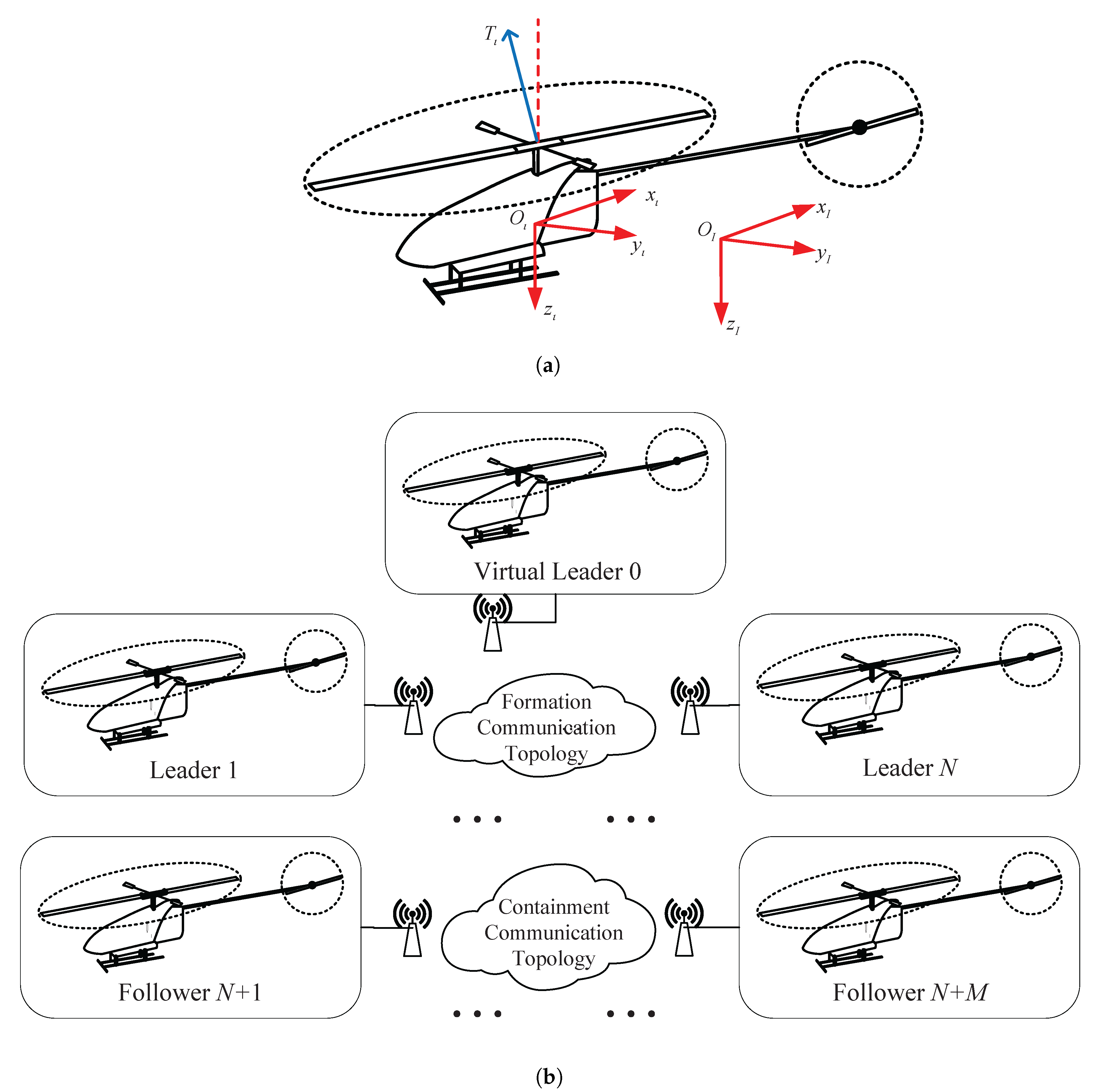
Figure 1a presents the spatial configuration of the inertial and body-fixed frames. As depicted in
Figure 1b, a flying system with
helicopters (including
N leaders and
M followers) is considered, where
is the set of serial numbers for the helicopters, and
and
are the sets of serial numbers for the leaders and followers, respectively. Also, the virtual leader is labeled as 0. The 6-DOF rigid body model of the
th UH is modeled as a position subsystem and an attitude subsystem as follows:
where
and
are the position and the velocity vectors of the inertial reference frame
, respectively.
and
denote the Euler angle and angular rate vectors of the body-fixed coordinate frame
, respectively.
is the unitary vector.
g indicates the gravity acceleration,
denotes the mass of UH, and
represents the diagonal inertia matrix. Further, the rotation matrix
, the anti-symmetric matrix
, and the rotational kinematic matrix
are defined below:
In translational dynamics, implies the force vector, with as the main rotor thrust controlled by the collective pitch . and denote the constants associated with the main rotor rotation speed and the collective pitch , respectively.
For the rotational dynamics,
is the moment vector applied to a helicopter, which is formed by
where
,
and
,
are the lateral and longitudinal wave motion coefficients of the main rotor.
denotes the damping coefficient of the yaw angle.
and
are damping coefficients related to the tail rotor and main rotor (e.g., rotation speed and blade radius).
is the collective pitch of the tail rotor.
and
denote the flapping angles of the main rotor along with the longitudinal and lateral axes, which are mainly controlled by longitudinal and lateral cyclic
and
. Their relationships can be approximated as
Therefore, combining Equations (3) and (4), a modified moment vector can be rewritten as
where
.
denotes the time constant of the main rotor. The parameters in the above matrices are
,
,
, and
, where the coefficients
,
and
,
can be obtained by the system model identification. The matrices
and
are given as
Remark 1. Note that the representations of force vector , moment vector , and blade flapping angles (both longitudinal and lateral ) are simplified in the above-mentioned model. The force and moment vectors generated by the main rotor, tail rotor, and fuselage can be highly complex due to unsteady aerodynamics and dynamic interactions. However, under steady or quasi-steady flight conditions (such as hover or low-speed cruise), these effects can be approximated using linearized or lumped-parameter models, significantly reducing computational complexity. Similarly, the blade flapping dynamics can be simplified under the small-angle assumption. In many control-oriented models, the flapping angles are approximated using first-order dynamics or even static gain relationships, assuming a linear response to cyclic pitch. These simplifications are reasonable in flight regimes, where the flapping angles remain small and high-frequency dynamics are negligible. Such simplifications keep a balance between model fidelity and computational efficiency, making them suitable for control design.
Remark 2. In this article, the virtual leader serves as a reference point that defines the desired trajectory and formation pattern for the actual leaders to follow and maintain. Although it does not physically exist, the virtual leader provides position or yaw angle information that coordinates the motions in the flying system. By tracking the virtual leader, each helicopter can maintain proper spacing and movement direction, thereby ensuring the overall geometric structure.
Let
,
,
and
be the actual input signal, which is combined with the collective pitch of the main and tail rotor, and the lateral and longitudinal cyclic. Each component plays a critical role in ensuring the helicopter’s stability and maneuverability. Due to the hydraulic or electrical malfunctions, and some environmental factors like extreme temperatures or corrosion, these control inputs may suffer from various types of faults. Among the most common are loss of effectiveness and bias faults, which allow the system to continue operating but with reduced performance. Such faults can result in sluggish or unresponsive control behavior, ultimately leading to degraded or even lost of control authority. In this article, the fault models are formulated as
where
,
, and
denote the partial loss of actuator effectiveness and the additional bias faults, respectively.
Subsequently, the flight dynamics (
1) and (
2) of the
th UH are separated into outer-loop (position) and inner-loop (attitude) subsystems for the control design. Since the design processes of three directions are similar, define
and
, and the outer-loop (position) subsystem can be rewritten as
where
,
and
are nonlinear functions.
and
imply the input signal to be designed and the lumped fault to be estimated, which are constructed as
and
Similarly, we denote
and
to reformulate the inner-loop (attitude) subsystem as
where
,
,
,
,
,
,
,
, and
are nonlinear functions.
and
denote the input signal and the lumped fault as follows:
and
Remark 3. It should be noted that the direct control inputs of the helicopter are , , , and . These inputs determine the control effectiveness in all flight directions and can be computed through the transformation relationships defined in (8) and (11). The above-mentioned (6) satisfies the following four cases: (1) When and , this indicates the fault-free (normal) case. (2) When and , it implies the partial loss of actuator effectiveness only. (3) When and , it indicates the bias fault only. (4) When and , it reveals both the partial loss of actuator effectiveness and bias faults. Note that when and , this refers to the stuck fault, i.e., sticks at a bounded function . However, this case cannot be compensated for by designing the AFTC scheme; thus, we only consider the other four cases in the subsequent sections. Before presenting the formation-containment control scheme, we make the following fundamental graph theory and some related lemmas, definitions, and assumptions.
The communication network among the
helicopters is represented by a directed graph
, where
is the node set and
is the edge set. The vertex sets of the leaders and the followers are defined as
and
, respectively. Consequently, we have
and
. The edge pair
means that the
ith UH can receive data from the
jth UH. The adjacent matrix
is a position matrix that can be defined as
when
, otherwise
. Denote the Laplacian matrix as
, where
,
, and
.
represents the degree matrix,
. Here, the Laplacian matrix is described as
where
signifies the communication topology among the leader UHs,
denotes the communication interaction from the leaders to the followers, and
implies the communication topology among the follower UHs.
In addition, , with being the connections between the ith leader UH and the virtual leader, where means that it can receive data from the virtual leader, or otherwise, .
Assumption 1 ([
32]).
As for the leader UHs, the virtual leader has at least one path to each leader UH. Also, there exists at least one path from the leader UHs to each follower UH. Lemma 1 ([
32]).
All the eigenvalues of matrix have positive real parts. Each entry of is positive and each row sum of is equal to 1. Definition 1 ([
32]).
(Convex Hull) Suppose that is a subset in the real vector space . The set is said to be convex if the point holds for any and arbitrary two elements α, β. The convex hull regarding a group of points in Z is the minimal convex set consisting of all points in X, and then, it is represented as . In this article, the control objective is to ensure the desired flight performance of
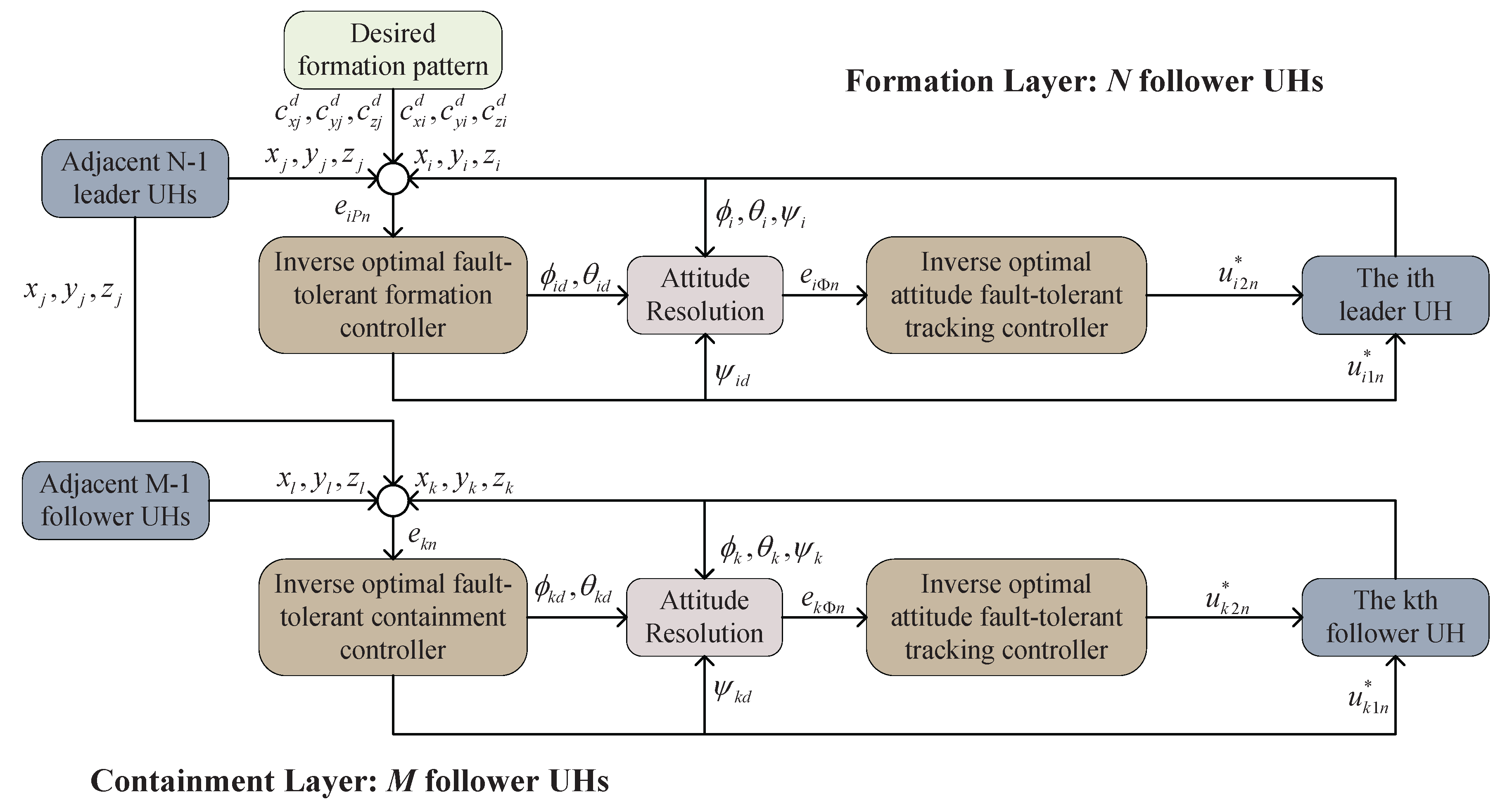
UHs. As shown in
Figure 2, a two-layer structure framework is employed to settle the inverse optimal fault-tolerant formation-containment control problem: one is the formation layer of
N leaders, and another is the containment layer of
M followers. Specifically, the leaders in the first layer can simultaneously take action and form a desired reference formation pattern, while the followers in the second layer are contained in a convex hull constructed by the leaders. Thus, the inverse optimal fault-tolerant control of the hierarchy-structured UHs is completed if and only if both two layers have achieved their own control objectives. That is, for
, there exists
and for
,
, there exists
where
is the position of the virtual leader.
is the relative position of the desired configuration between the
ith leader UH and the virtual leader.
Remark 4. Owing to the under-actuated mechanics of the ιth UH, the proposed control algorithm is separated into two cascaded control modules. The outer-loop (position) controller calculates the input signal and appropriate attitude commands and to navigate the helicopter along the target trajectories. It can be calculated that and areand with denotes the yaw angle of the virtual leader. Then, the command is delivered to the inner-loop (attitude) controller that calculates . Assumption 2 ([
33]).
The position and the yaw angle reference from the virtual leader and their derivatives are bounded and continuous functions. Assumption 3 ([
7]).
The Euler angle vectors (i.e., roll angle , pitch angle , and yaw angle ) are bounded and satisfy , and for all t. Lemma 2 ([
30]).
(Inverse Optimal Control) Consider a nonlinear system as follows:where and denote the state and control input vectors, while and are the smooth functions. If there exist a positive-definite control Lyapunov function , and a control strategy stabilizing the whole system (17), then we have , where is the inverse optimal control input for the system (17), and the minimized performance index function iswhere with and . Lemma 3 ([
7]).
(Neural Network Approximation) For an unknown nonlinear function , there is a neural network satisfying the following condition:where represents the ideal neural network weight matrix, denotes the activation function, and depicts the approximation error bounded by . In this article, is assumed as the Gaussian function, i.e., , where represents the width, and , with μ as the node number. 4. CL-Based Inverse Optimal Fault-Tolerant Containment Controller
As for the second layer, the optimal position containment controller and optimal attitude tracking controller are separately designed for each follower UH in this subsection. Based on this, the followers will approach the convex region constructed by the leaders.
Firstly, the containment error
and the tracking error
of the
kth helicopter are defined as
and
where
k,
,
,
, and
are the connective relation between the
kth follower and the
lth follower or the
jth leader.
.
and
denote the virtual controller to be designed.
Next, the entirety of the CL-based inverse optimal control schemes with fault compensation design for the follower UHs are presented in the subsequent steps.
For the outer-loop (position) subsystem, differentiating
yields
where
. Furthermore, we design the following feedforward virtual controller
for target enclosing:
where
is a positive constant and has
.
Similarly, the CL-based fault estimation observer
with the adaptive learning law of network weight
is constructed as
where
,
, and
are positive constants.
is the prediction error with
, with
as a positive constant.
and
are the estimation errors of network weight and lumped faults.
Then, the derivative of
is rewritten as
where
.
Similarly, for the inner-loop (attitude) subsystem, the time-derivation of
is calculated as
, and then, the virtual controller is
where
is a given positive constant, and the neural network weight
is formed by
where
and
are positive constants.
denotes the prediction error with
, with
as a positive constant.
Combining (71) and (70), the time-derivative of
has the form
where
is the approximation error of the network weight.
By differentiating
with respect to the time, we obtain
; then, the CL-based fault estimation observer with the network weight training law is formulated as
where
,
and
denote the positive constants.
is the prediction error with
. Also,
and
are the approximation errors.
Then, we have
where
.
Theorem 3. Under the designed virtual controllers (66) and (70), the fault estimation observers (67) and (73) with the updating laws of network weights (68), (71), and (74), the inverse optimal fault-tolerant controllers and are designed with the positive constants and :which can make the tracking errors , , , and , as well as the errors , , , , , , , and approach a small region of the origin and achieve the minimum cost functions as follows:where , . , and . Proof of Theorem 2. For the outer-loop (position) subsystem, select the Lyapunov function as follows:
By employing the aforementioned procedures in (
32)–(
39), we can know that for a given
,
becomes
where
.
,
, and
are positive constants satisfying
and
. Note that if the conditions
,
and
hold, it follows that the controller
can ensure that the following condition holds:
where
and
. From Lemma 2, when
, the CL-based inverse optimal controller
can minimize the cost function (
78). Moreover, the tracking errors
and
along with the estimation errors
,
, and
will converge to a small region around the origin. Then, the inverse optimal fault-tolerant controller is designed as (
76).
For the inner-loop (attitude) subsystem, the Lyapunov functional is chosen as
and we can know that, if
, we have
where
.
,
, and
are positive constants satisfying
and
. This means that if the inequalities
,
,
,
, and
hold, the controller
can stabilize the whole subsystem such that
where
,
and
. Moreover, the tracking errors
and
alongside the errors
,
,
,
, and
approach a small neighborhood of the origin.
The containment tracking objective is illustrated as follows. From (
15), the containment error is described as
, where
,
. In terms of the condition (
63), it has
, and the following equation can be derived:
where
, which can be written as
, i.e., the containment objective is achieved accordingly. □
Remark 6. For the flying system containing N leaders and M followers, if we choose the Lyapunov function as , it derives that with and , and the inverse optimal fault-tolerant controller , , and , can minimize the cost function .
Remark 7. Among the above-mentioned parameters, larger values of , , , , , , and along with smaller values of , , , , , , and can be chosen such that , , , , , , and hold, keeping a balance between the faster control convergence time/rate and the input characteristic.
5. Simulation Results
The flight performance of the inverse optimal fault-tolerant formation-containment control protocol was examined using a numerical example. A UH system composed of three leaders and two followers were considered. This leader-following platoon was supposed to accomplish a fault reconfiguration mission, changing from arbitrary positions in the air to an assigned pattern. The related physical parameters of each UH are given in
Table 1.
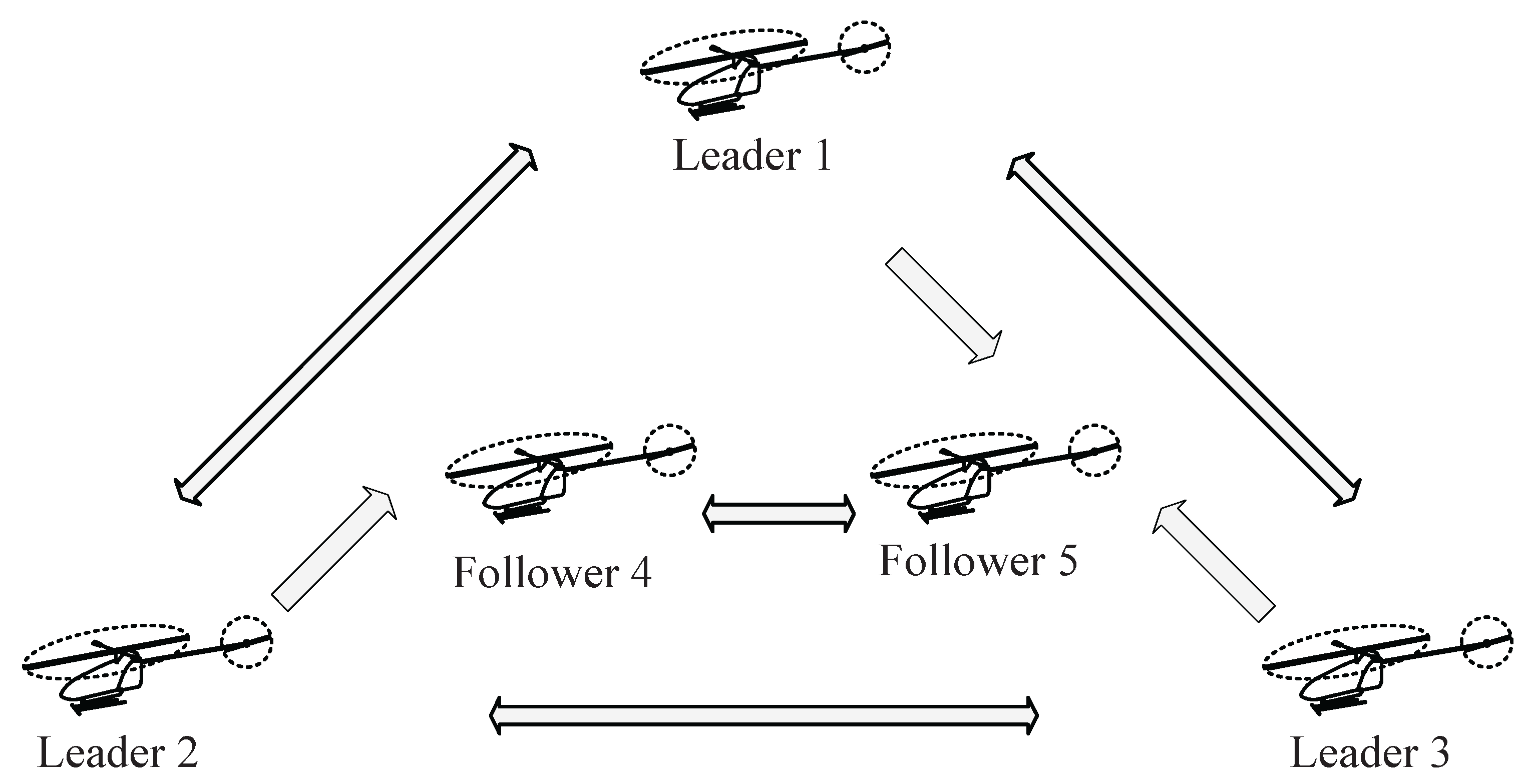
The control objective of this theoretical case analysis is to enable three leaders (labeled as 1, 2, and 3) to maintain a triangle formation and encircle around a particular target or reference provided by a virtual leader. Afterward, the position trajectories of two followers (labeled as 4 and 5) need to be entered into the convex hull spanned by the leaders. The information transmission topology among members in the helicopter system is exhibited in
Figure 3. The reference trajectory of the virtual leader can be expressed as
,
,
, and
, and a desired formation pattern of leaders is set with the relative distances as
,
,
,
,
,
and
with
.
The other related simulation parameters are given as
,
,
,
,
,
,
,
,
,
,
, and
. The faults are assumed to occur in leaders 2 and 3 and follower 5, while the others operate under normal conditions. The detailed fault parameters are set as follows:
Under the initial conditions of
,
,
,
, and
, the simulation results are provided in
Figure 4,
Figure 5,
Figure 6,
Figure 7,
Figure 8 and
Figure 9.
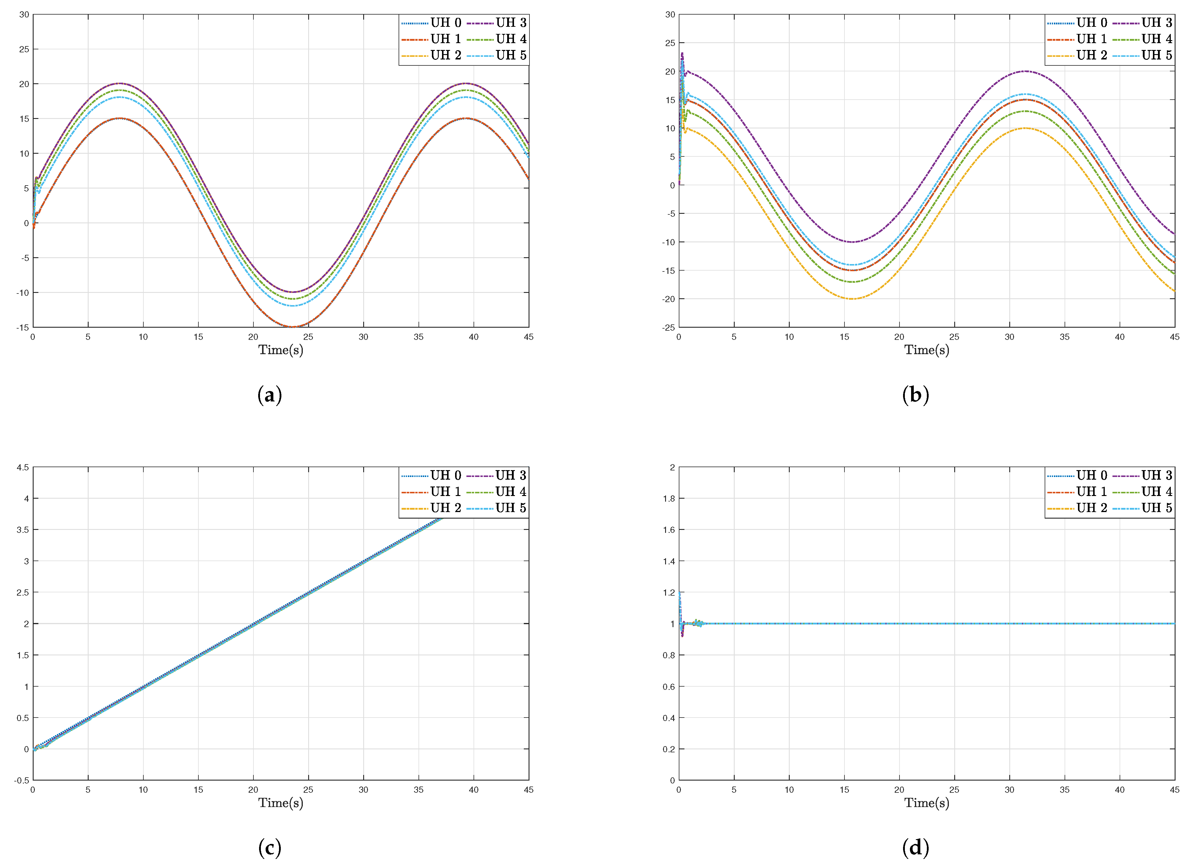
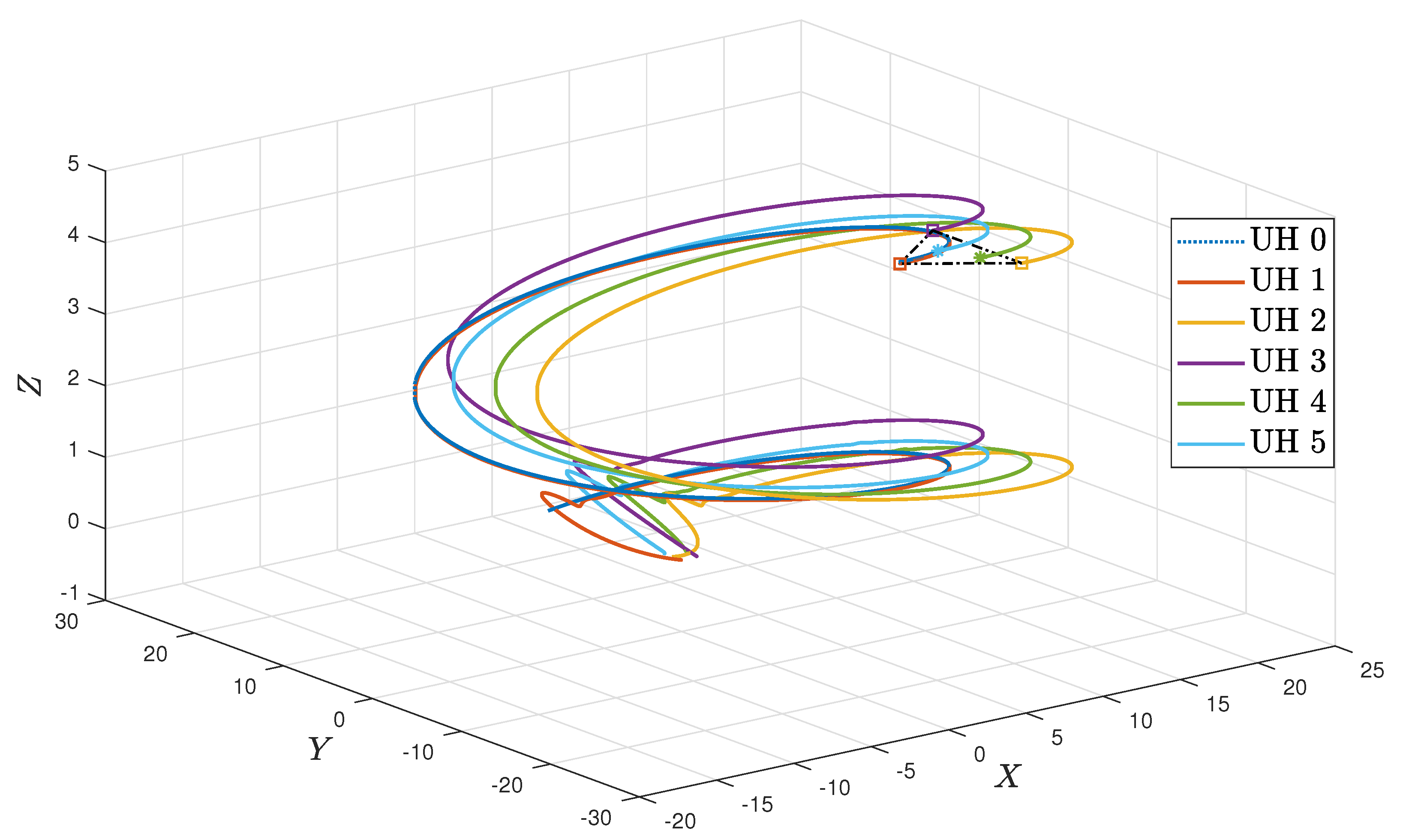
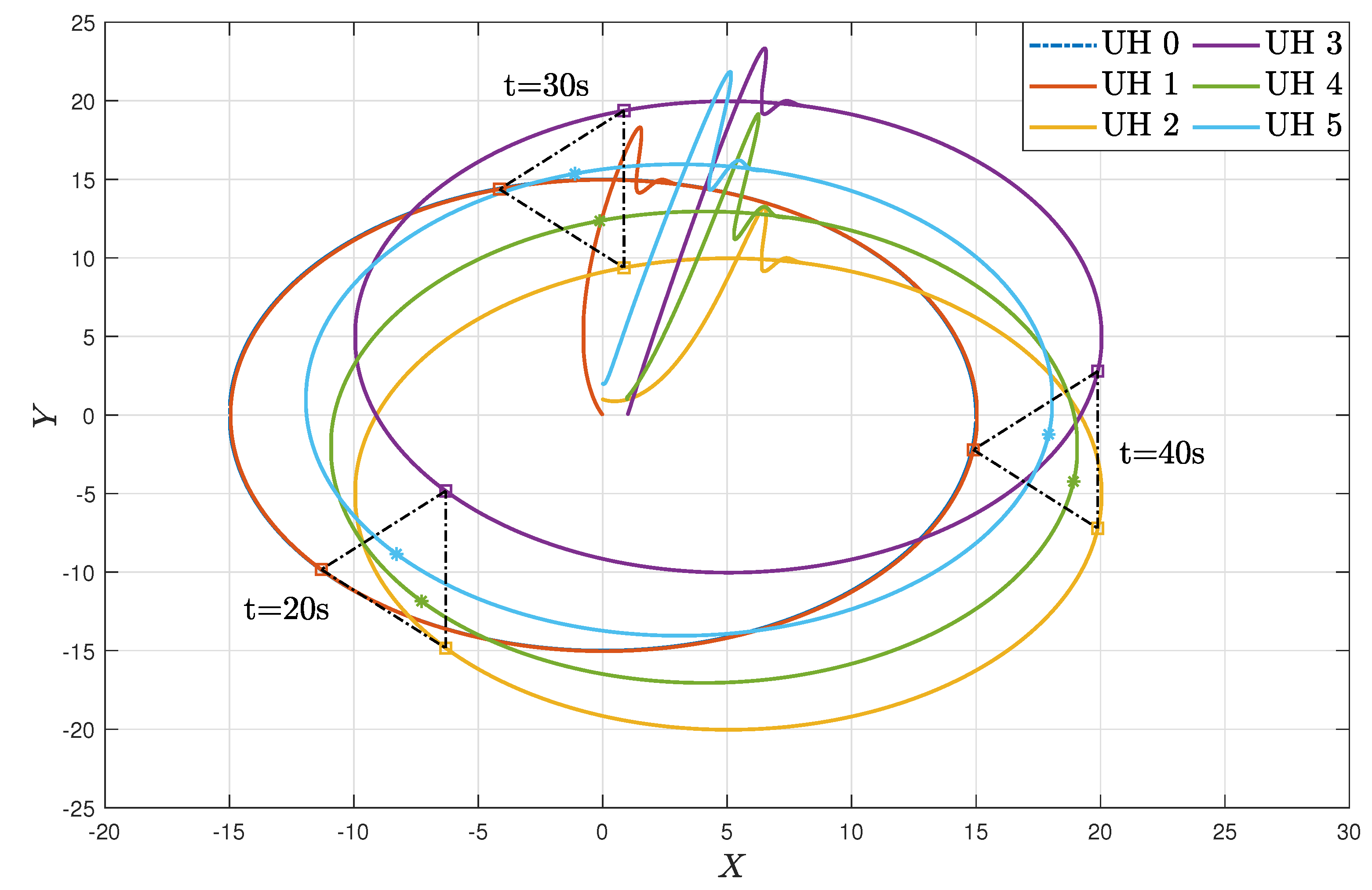
Figure 4a–d show the moving trajectories (i.e.,
,
,
, and
) of the five UHs.
Figure 5 depicts the formation-containment performance in the 3-orthogonal plane.
Figure 6 depicts the formation-containment performance in the XY plane. From this, it can be concluded that the designed protocol can simultaneously make the multi-UHs reach and preserve the target geometric pattern from any position and track the global reference signal by a virtual leader with a specific position. In
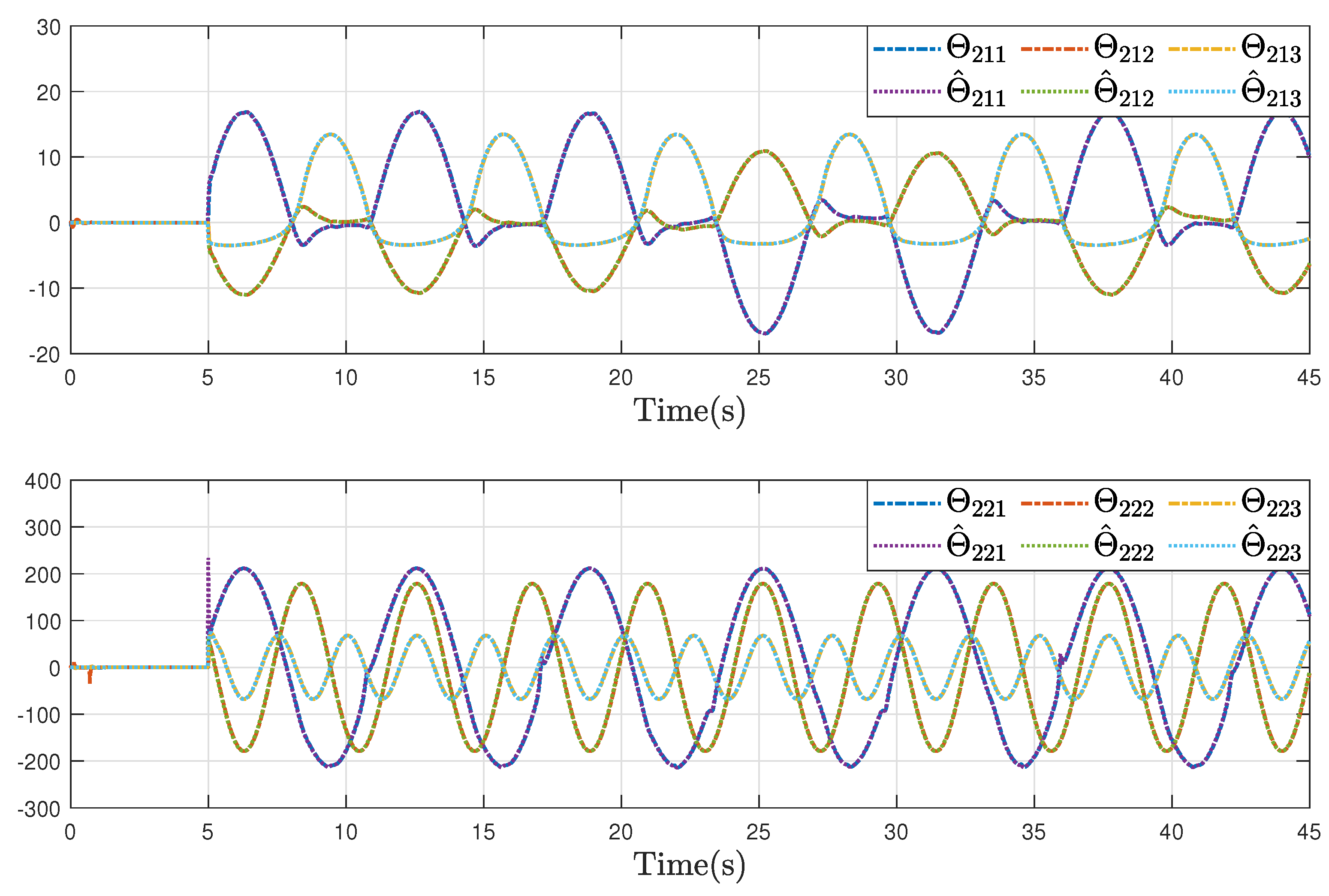
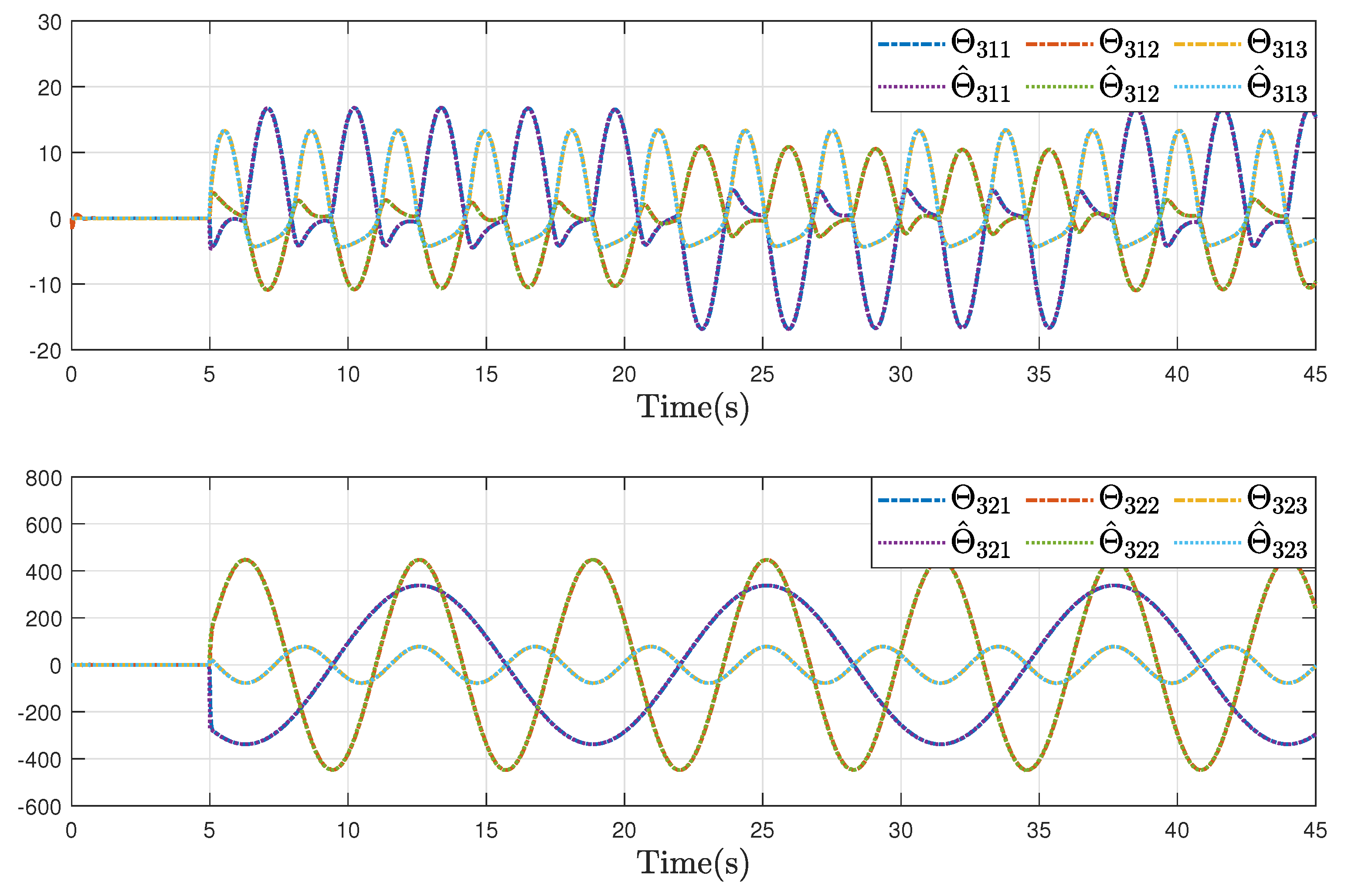
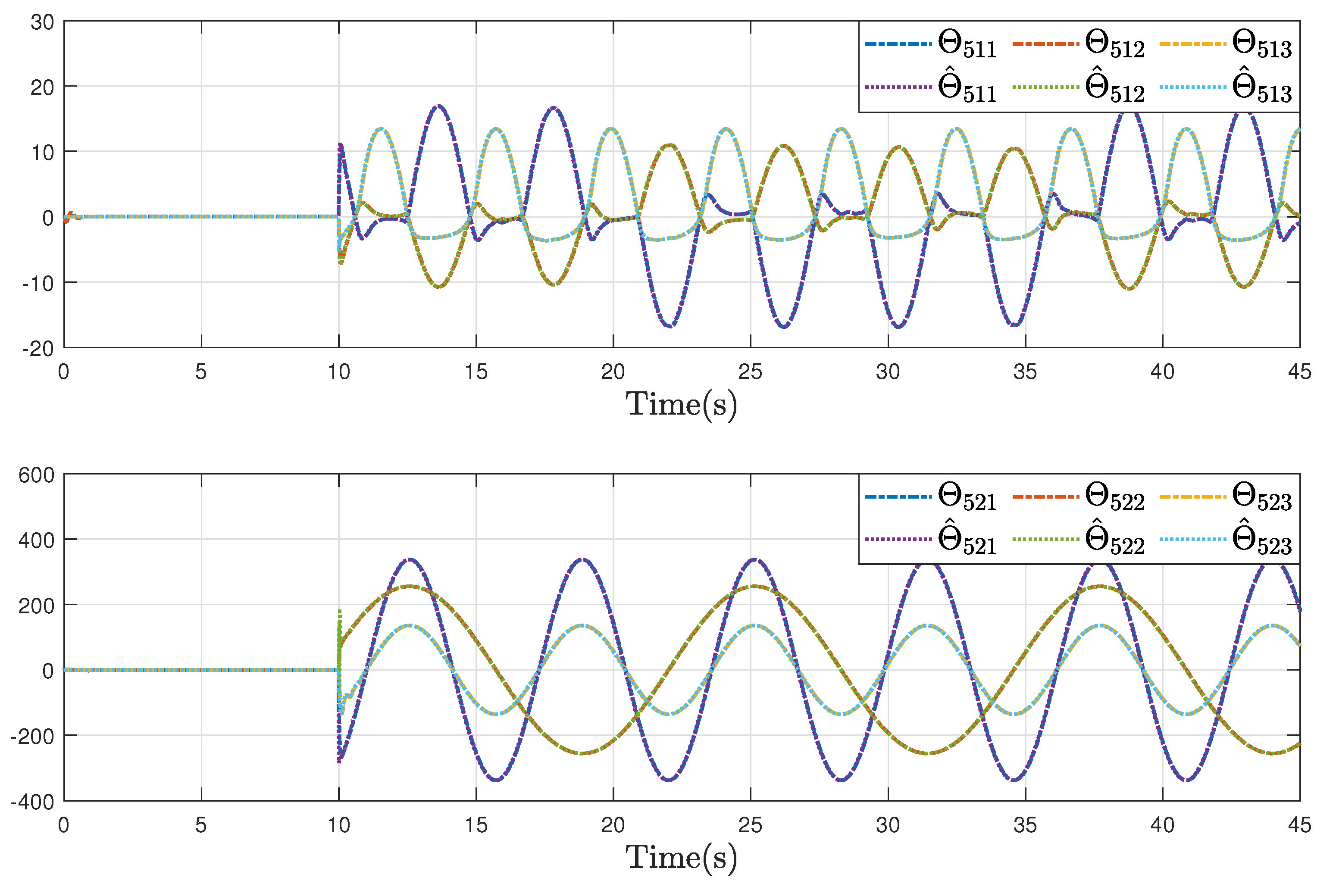
Figure 7,
Figure 8 and
Figure 9, it can be observed that the proposed fault estimation observer will approximate the lumped actuator faults
,
,
,
,
, and
well even though the faults occur. Through the above analysis of these helicopter formations and containment statuses, we can conclude that the system realizes the expected formation-containment flight performance under the designed inverse optimal fault-tolerant control protocol, and the fault effects can be compensated well based on the relevant estimations.
Further, to validate the advantages of the proposed inverse optimal fault-tolerant formation-containment control strategy, comparative results were conducted under the same initial conditions and parameters. Specifically, two schemes were considered: one using a non-optimal control law (Case I, i.e.,
and
), and the other omitting the serial-parallel estimation model (Case II, i.e.,
,
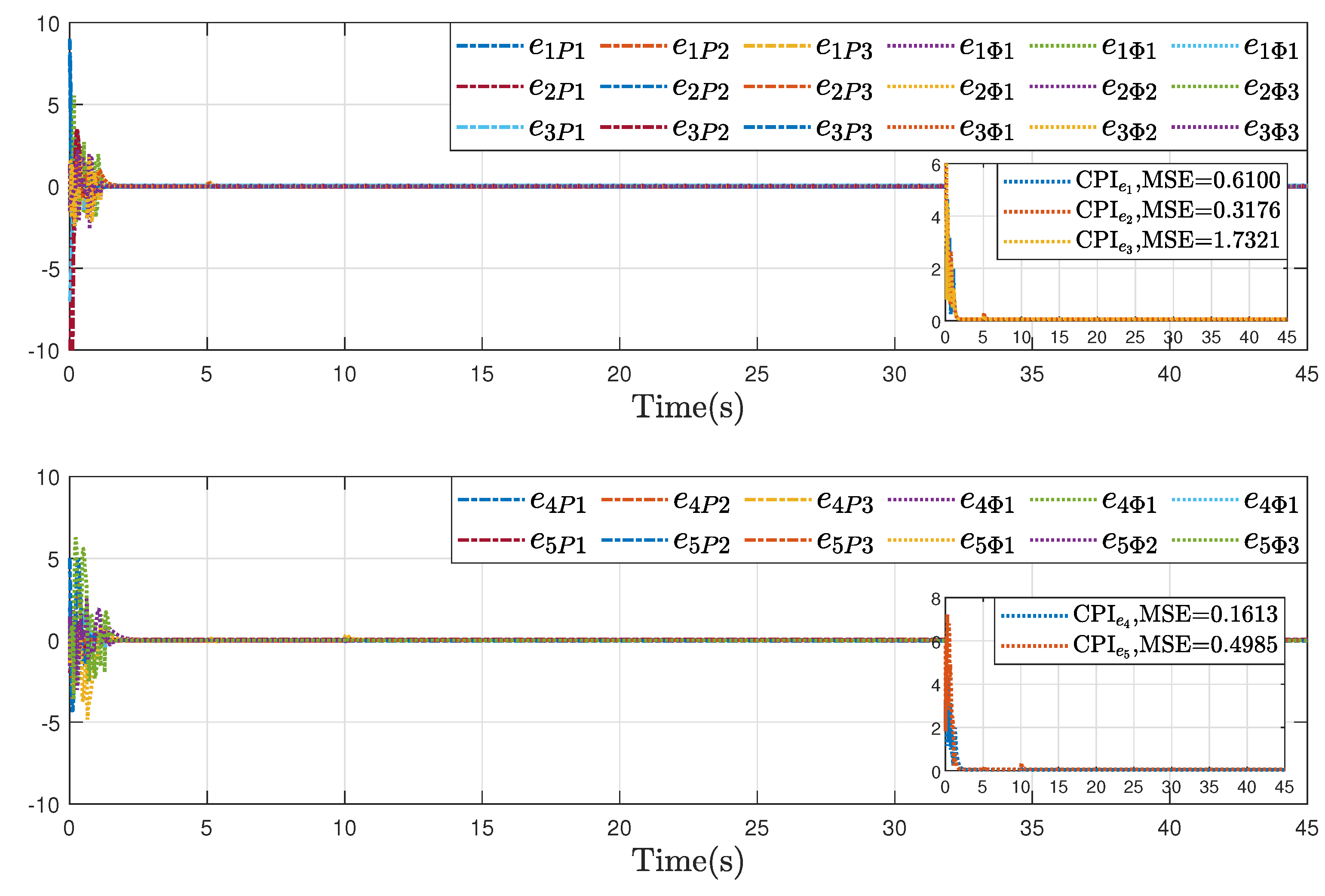
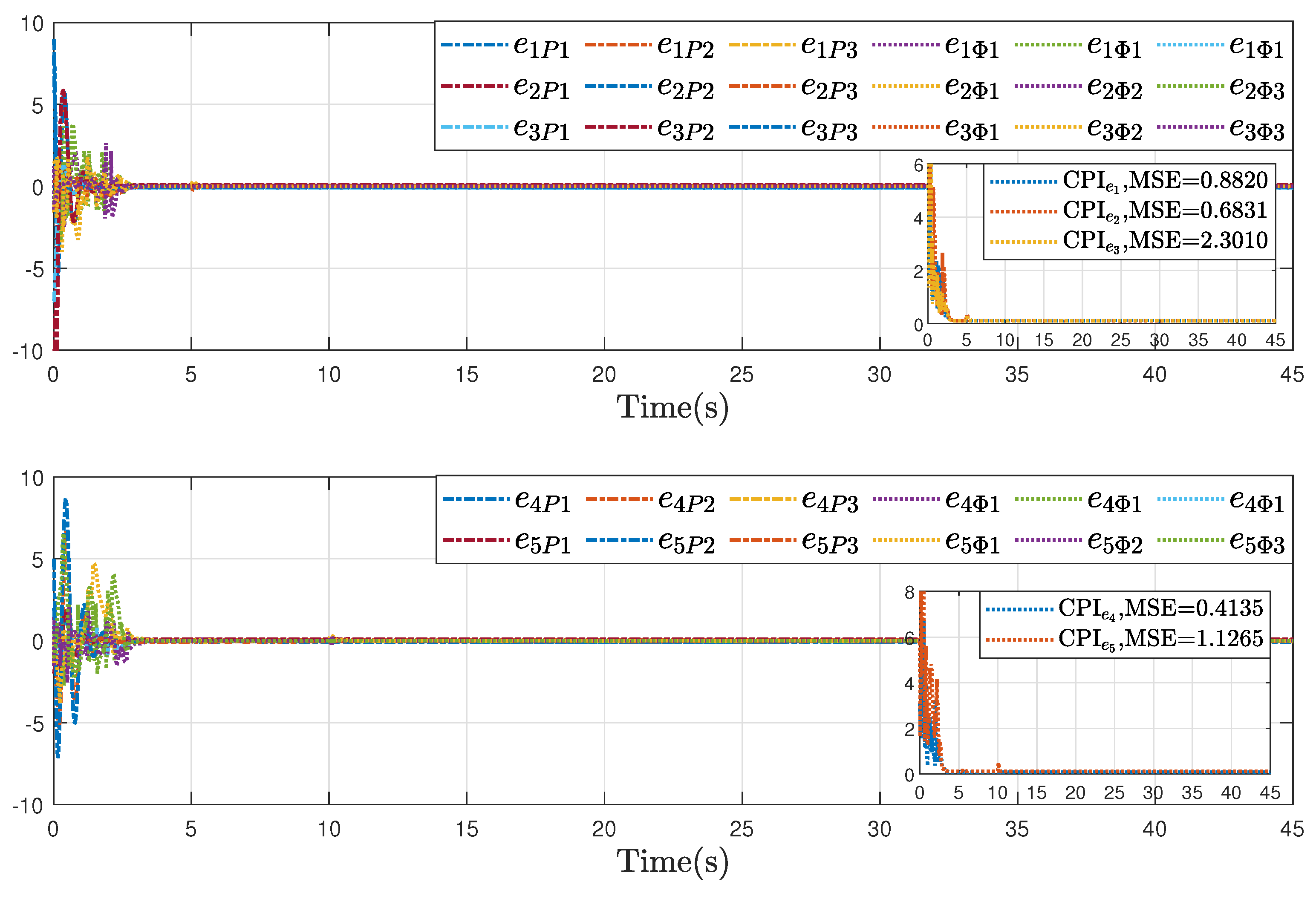
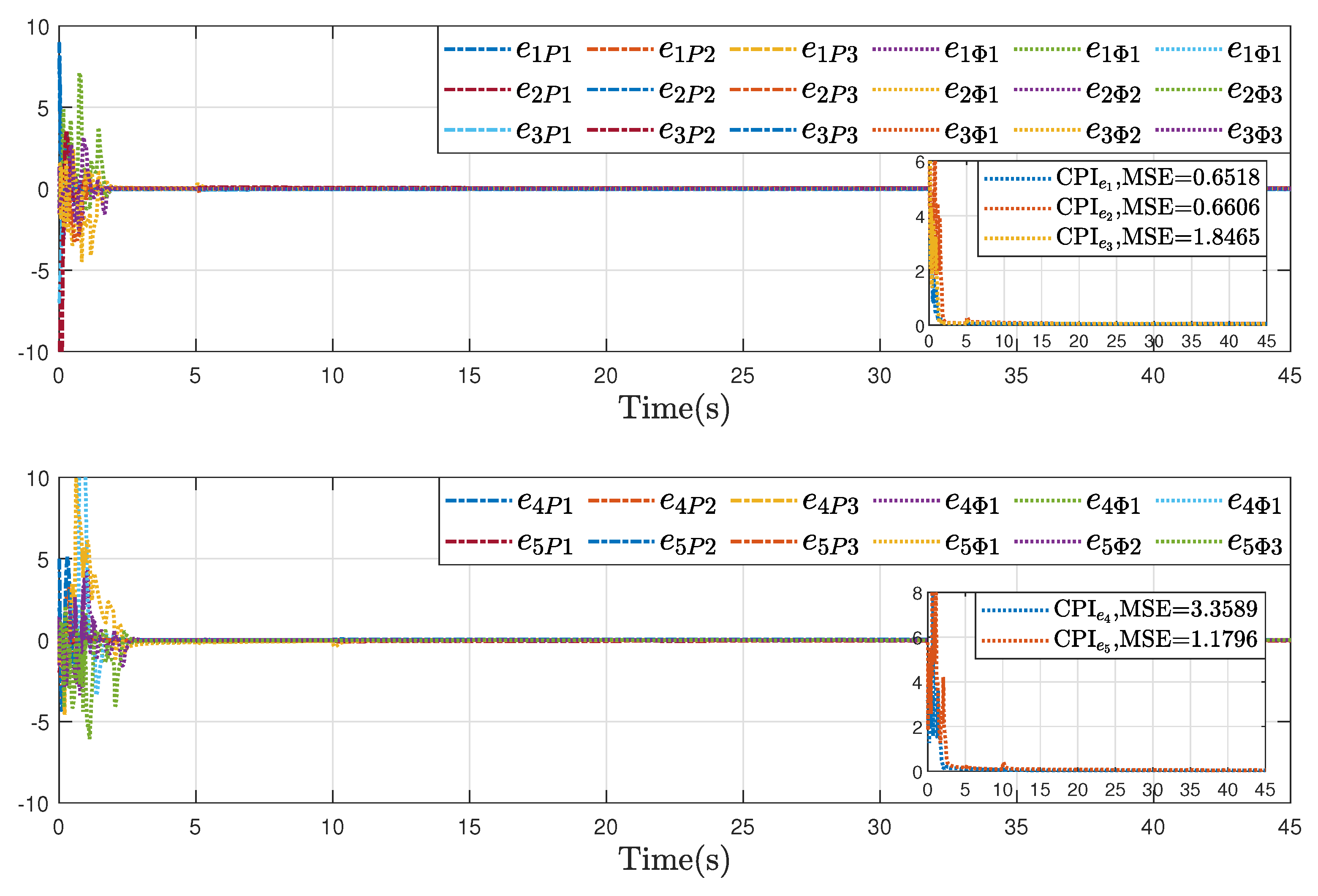
). The corresponding formation error
and containment error
are presented in
Figure 10,
Figure 11 and
Figure 12, where
Figure 10 presents the performance of the proposed inverse optimal fault-tolerant formation-containment control strategy,
Figure 11 displays the error trajectories under Case I while
Figure 12 shows its performance. As illustrated, the proposed control protocol improves the tracking accuracy in both formation and containment tasks, compared with Case I and Case II. These improvements highlight the optimality and accurate estimation in enhancing system performance.
To quantitatively evaluate control performance, two reliability indices are introduced: the comprehensive performance index (CPI), defined as , and the mean-squared error (MSE), given by . The calculation results of these reliability indices also illustrate the effectiveness and the superiority of our proposed control algorithms on formation-containment flight.


