A Visual Guidance and Control Method for Autonomous Landing of a Quadrotor UAV on a Small USV

Abstract

Unmanned Surface Vehicles (USVs) are commonly used as mobile docking stations for Unmanned Aerial Vehicles (UAVs) to ensure sustained operational capabilities. Conventional vision-based techniques based on horizontally-placed fiducial markers for autonomous landing are not only susceptible to interference from lighting and shadows but are also restricted by the limited Field of View (FOV) of the visual system. This study proposes a method that integrates an improved minimum snap trajectory planning algorithm with an event-triggered vision-based technique to achieve autonomous landing on a small USV. The trajectory planning algorithm ensures trajectory smoothness and controls deviations from the target flight path, enabling the UAV to approach the USV despite the visual system’s limited FOV. To avoid direct contact between the UAV and the fiducial marker while mitigating the interference from lighting and shadows on the marker, a landing platform with a vertically placed fiducial marker is designed to separate the UAV landing area from the fiducial marker detection region. Additionally, an event-triggered mechanism is used to limit excessive yaw angle adjustment of the UAV to improve its autonomous landing efficiency and stability. Experiments conducted in both terrestrial and river environments demonstrate that the UAV can successfully perform autonomous landing on a small USV in both stationary and moving scenarios.

1. Introduction

River inspection is a challenging task, especially in urban areas with extensive and intricate river networks. Traditional manual inspection methods are not only inefficient but also limited in coverage, often being affected by factors such as terrain conditions, weather, and safety concerns [1,2]. Unmanned Aerial Vehicles (UAVs) play a crucial role in heterogeneous cooperation tasks due to their high mobility and aerial perspective, providing real-time situational awareness [3]. However, given the limited battery capacity of UAVs, docking stations are required for recovery during missions. In the narrow rivers of urban areas, small USVs offer advantages such as excellent maneuverability and long endurance, making them ideal for use as docking stations [4]. By combining the strengths of UAVs and USVs, a heterogeneous cooperative system can be formed that enhances autonomous river inspection capabilities [5,6].

In the context of UAV landing on a USV, traditional methods typically involve manual control of the UAV using video feedback from the onboard camera [7]. However, this approach has limitations, as the operator’s restricted FOV and lack of overall environmental awareness make it challenging to effectively control the UAV, particularly in dynamic river environments with obstacles. With the advancement of navigation technology, various methods have emerged to meet different application requirements, offering more options for UAV autonomous landing research. In addition to Global Navigation Satellite System (GNSS)-based navigation methods, techniques utilizing remote sensors and vision-based methods have been widely applied in this field.

Ultra-Wide-Band (UWB)-based guidance techniques offers advantages such as low power consumption and reliable performance in various weather conditions, making them suitable for UAV autonomous landing in outdoor environments [8]. Zeng et al. [9] achieved UAV autonomous landing by placing four UWB anchors on a mobile platform and two UWB tags on the UAV for guidance, with IMU data integrated to enhance localization accuracy. Ochoa et al. [10] used extended Kalman filtering to estimate the positions of two UWB tags on the UAV, aiming to reduce the localization error in the UWB-based landing assistance system. However, experimental results have shown that the positioning accuracy of UWB-based methods is affected by distance and that UWB signals are susceptible to interference from conductive materials [11]. As a result, the effectiveness of this method is limited in narrow river environments with obstacles and floating debris.

To guide the UAV in approaching the USV and achieving autonomous landing in narrow river environments, it is necessary to plan the flight path for the UAV. Traditional path search algorithms, heuristic algorithms, and machine learning-based approaches are commonly used for path planning [12]. Demiane et al. [13] proposed a UAV trajectory planner in which the target waypoints are determined based on the Received Signal Strength Indicators (RSSI) signal. The UAV trajectory is then optimized using a two-option heuristic solution for the Traveling Salesman Problem (TSP), which minimizes travel distance while ensuring prioritized coverage of critical areas. However, flight paths with sharp turns do not consider the feasibility of UAV motion. Maintaining continuous UAV motion and avoiding stops during turns can reduce energy losses caused by frequent acceleration and deceleration; however, it is necessary to plan a smooth trajectory for guidance. Shao et al. [14] designed a cooperative UAV–USV autonomous landing platform equipped with ultrasonic ranging devices for positioning. A hierarchical landing guide point generation algorithm was proposed based on ultrasonic range and decreasing height, which were then used to construct a trajectory based on the cubic B-spline curve, guiding the UAV for smooth landing. However, this method is limited by the ultrasonic signal strength, which restricts the autonomous landing range. Additionally, it is only applicable in an obstacle-free environments, as obstacles can affect trajectory planning due to blocking or reflection of the ultrasonic signals. Ji et al. [15] developed a framework for aerial perching on moving inclined surfaces. In their approach, the terminal states and trajectory durations are adjusted adaptively rather than being predetermined. Additionally, SE(3) motion planning is employed to prevent premature contact with the landing platform. Localization of the UAV and landing platform are based on an indoor motion capture system. These methods were validated through experiments, demonstrating that the planner can generate optimal trajectories within 20 ms and re-plan with a warm start in just 2 ms. Based on the above paper, Gao et al. [16] built a fully autonomous tracking and perching system with solely onboard sensors instead of relying on external perception facilities. To validate their proposed approach, extensive real world experiments were conducted. The drone successfully tracked and perched on the top of an SUV at 30 km/h and entered the trunk of the SUV at 3.5 m/s with a 60 degree incline. However, real-time trajectory planning requires high computational resources which can increase system complexity and costs, making implementation challenging for UAVs with limited hardware. Furthermore, although effective in controlled environments or with motion capture, the performance of such systems may decline in real-world conditions.

Vision-based methods offer advantages such as real-time performance and high accuracy. Specifically, detection methods using artificial fiducial markers have been adopted in many studies [17]. R. Polvara et al. [18] proposed a vision-based approach for UAV autonomous landing on a USV in a Gazebo simulation environment by using a fiducial marker placed on the USV to estimate its attitude. Additionally, an extended Kalman filter was employed to ensure that attitude information could still be obtained when the marker was not visible. With this method, the UAV can adjust its own attitude during the landing process to align with the USV’s state, preventing collisions between the UAV and USV. Y. Park et al. [19] designed a recursive fiducial marker [20] based on the ArUco fiducial marker, enabling the UAV to detect the marker at various distances. An extended Kalman filter was used to estimate the marker’s position, reducing control instability during the UAV’s vertical descent caused by the loss of marker visibility. Xu. et al. [21] constructed a landing platform on a USV and placed a recursive fiducial marker above it, enabling the UAV to land on the moving USV based on visual tracking. Although vision-based detection using fiducial markers offers the advantage of high recognizability, the onboard camera may fail to detect the marker when the UAV is far from the marker or the marker size is small. As a result, the range of autonomous landing is limited by the marker’s size in the camera image. Moreover, horizontally placed markers are susceptible to interference from lighting and shadows in outdoor environments, which can affect the detection of the marker and undermine the UAV’s autonomous landing performance.

T.M. Nguyen et al. [22] integrated the UWB and vision-based approaches, using UWB positioning for initial guidance in autonomous landing to compensate for the distance limitations imposed by the small FOV in vision-based systems. According to the experimental results, although the proposed method can achieve the intended goal, the UAV’s flight trajectory demonstrates considerable fluctuations. O. Procházka et al. [23] employed Model Predictive Control (MPC) to plan the UAV’s autonomous landing trajectory considering both the dynamic constraints and state estimation of the UAV, achieving attitude synchronization between the UAV and USV during the landing process. In addition to state estimation based on the model itself, the authors placed an AprilTag fiducial marker and UV LEDs on the USV for real-time state estimation. However, both simulation and experimental results indicated prolonged flight time and long adjustment times for both position and attitude tracking. Furthermore, in real-world experiments the UAV exhibited a notable steady-state error during the landing process.

In summary, most studies on UAV autonomous landing using visual guidance rely on horizontally placed fiducial markers, which are detected by the onboard camera to guide the UAV’s descent toward the landing platform. However, horizontally placed markers are prone to interference from lighting conditions, which can affect marker recognition in outdoor environments. Moreover, due to the limited range of visual perception, relying solely on visual guidance becomes challenging when the UAV is far from the USV. In terms of UAV guidance, methods based on remote sensors often have limited effective ranges, making it difficult to achieve successful autonomous landing on narrow and intricate rivers with nearby obstacles. In this study, an autonomous approach and landing method for a quadrotor UAV on a small USV is proposed by incorporating an improved minimum snap trajectory generation algorithm [24] with a visual guidance and control method based on an event-triggered mechanism. The main contributions of this paper are summarized as follows:

• An improved minimum snap trajectory planning algorithm is proposed to refine the flight trajectory based on given waypoints, ensuring trajectory smoothness while keeping the deviation between the generated trajectory and the target flight path within an acceptable range. This guides the UAV in approaching the USV in narrow river environments while improving flight stability during trajectory tracking and reducing energy consumption caused by frequent velocity changes.
• Based on a small USV adapted for operating in narrow rivers, a landing platform with a vertically placed fiducial marker is designed to separate the UAV landing area from the fiducial marker detection region in order to mitigate the interference from lighting and shadows on the fiducial marker. Additionally, an event-triggered visual guidance and control method is introduced to enhance UAV stability by optimizing heading and position control during the autonomous landing process.
• An autonomous landing system is developed comprising a USV, quadrotor UAV, and wireless ground station. The system design involves both hardware setup and software development. Outdoor experimental results show that the proposed method enables stable and autonomous landing of a UAV on a small USV, demonstrating the feasibility of the PX4 and ROS2 systems.

2. System Modeling

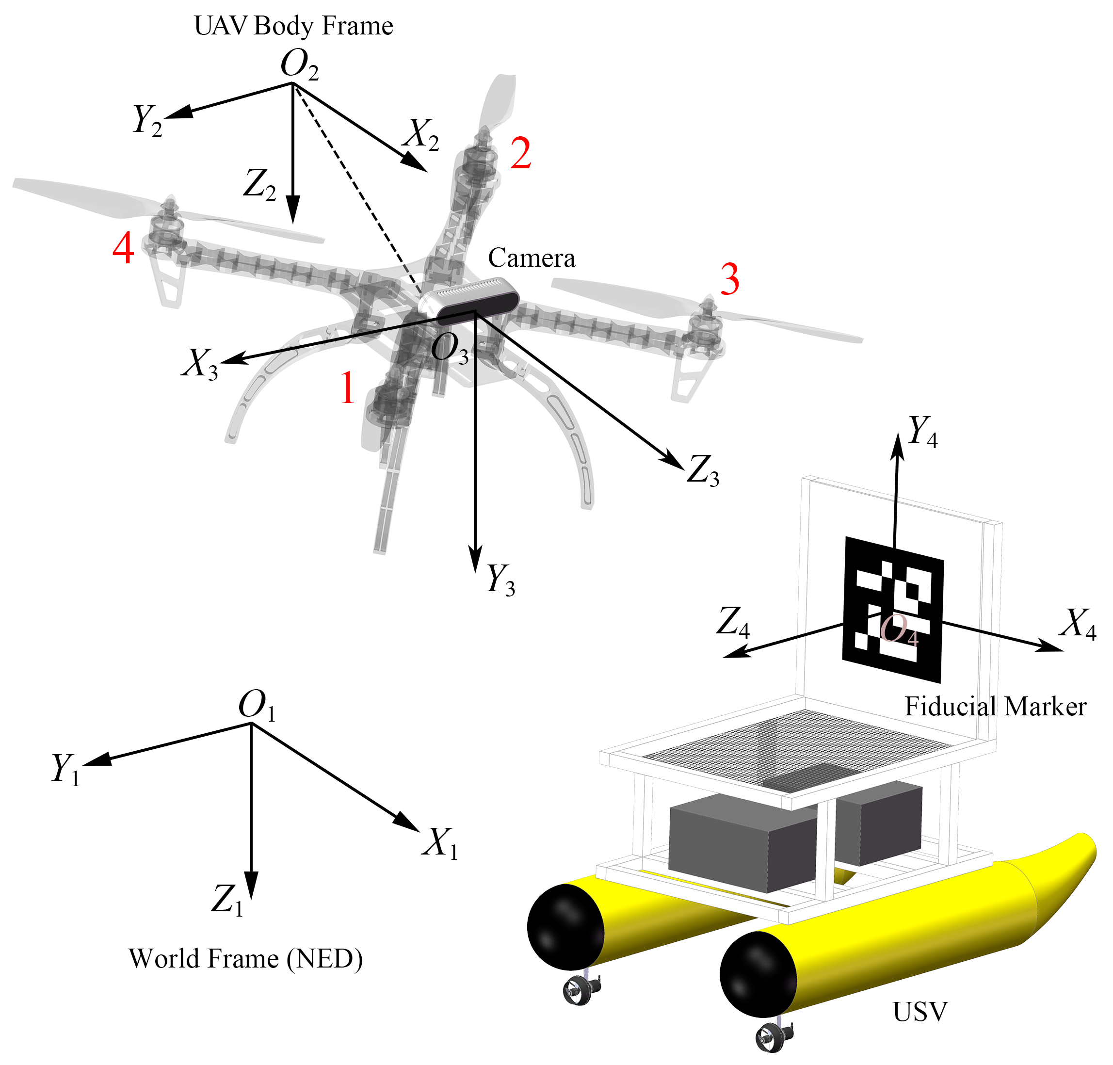
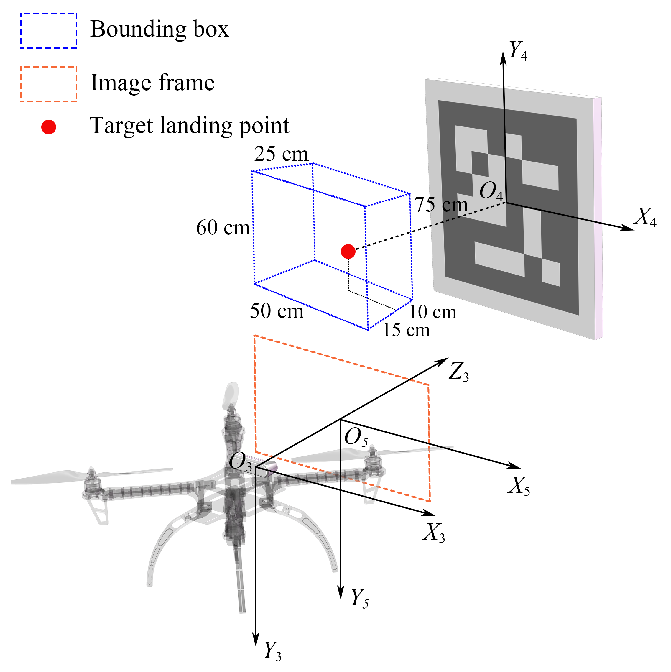
2.1. Coordinate System Definition

As shown in Figure 1, the world frame $\mathcal{W}$ is denoted by $O_1{X}_1{Y}_1{Z}_1$, defined as a North–East–Down (NED) frame. The UAV body frame $\mathcal{B}$ is denoted by $O_2{X}_2{Y}_2{Z}_2$ and located at the UAV’s center of mass. The $O_2{X}_2$ and $O_2{Y}_2$ axes lie on the propeller plane of the UAV, while the axis $O_2{Z}_2$ is perpendicular to this plane and oriented downwards. The axis $O_2{X}_2$ is oriented along the bisector of the angle formed by the first and third arms of the UAV, aligning with the UAV’s heading. The camera frame $\mathcal{C}$ for the UAV is defined as $O_3{X}_3{Y}_3{Z}_3$ in the Forward–Right–Down (FRD) configuration. The optical axis, represented by $O_3{Z}_3$, aligns with the axis $O_2{X}_2$. The ArUco fiducial marker coordinate frame $\mathcal{A}$ is denoted as $O_4{X}_4{Y}_4{Z}_4$ and follows a Forward–Left–Up (FLU) configuration, with its origin at the center of the marker. From a viewpoint behind the marker and looking forward, the $O_4{Y}_4$ axis points upward, the $O_4{X}_4$ axis points to the left, and the $O_4{Z}_4$ axis points forward.

2.2. UAV Dynamics Model

In this article, we use the UAV dynamics model proposed by [25] for reference. The direction of the thrust f generated by the four propellers is along $-O_2{Z}_2$. The translational motion of the UAV depends on the gravitational acceleration g and thrust f. Given the position $\mathbf{p}={[p_x,p_y,p_z]}^{\mathrm{T}}\in {\mathbb{R}}^3$ of the UAV in $\mathcal{W}$ and the rotation matrix ${\mathbf{R}}_{\mathcal{B}}^{\mathcal{W}}\in \mathbf{so}\left(3\right)$ from $\mathcal{B}$ to $\mathcal{W}$, the simplified model of the quadcopter dynamics can be written as follows:

$$\left\{\begin{array}{c}\ddot{\mathbf{p}}=g{\mathbf{e}}_3-f/m{\mathbf{R}}_{\mathcal{B}}^{\mathcal{W}}{\mathbf{e}}_3\hfill \\ {\dot{\mathbf{R}}}_{\mathcal{B}}^{\mathcal{W}}={\mathbf{R}}_{\mathcal{B}}^{\mathcal{W}}\widehat{\Omega }\hfill \end{array}\right.$$

(1)

where ${\mathbf{e}}_3={[0,0,1]}^{\mathrm{T}}\in {\mathbb{R}}^3$ and $\widehat{\Omega }:{\mathbb{R}}^3\to \mathbf{so}\left(3\right)$ is the skew-symmetric matrix form of the UAV body rate $\Omega \in {\mathbb{R}}^3$, while g represents the gravitational acceleration and m is the mass of the UAV.

2.3. Finite State Machine

The UAV flight process is divided into the following three stages, which the Finite-State Machine (FSM) uses to determining the UAV’s behavior:

• Idle: This is the initial stage of the system. The UAV hovers in the air, waiting for further commands. After receiving the landing command from the ground station, the system transitions to the Approaching stage.
• Approaching: At the beginning of the Approaching stage, the UAV automatically computes an optimized trajectory based on desired waypoints, then initiates trajectory tracking. When the UAV’s front-facing camera detects the fiducial marker on the landing platform, the state automatically switches to the Landing stage.
• Landing: In this stage, the UAV approaches the landing platform based on visual guidance. When the relative pose error between the UAV and the ArUco fiducial marker falls below the threshold value, the motors are shut down and the UAV falls onto the landing platform, completing the landing.

3. Trajectory Generation

3.1. Cost Function and Constraints

The trajectory of each segment $\in {\mathbb{R}}^3$ separated by waypoints is represented by three independent seventh-order polynomials for each axis in three-dimensional space, describing the UAV’s target position along each axis as a function of time t. The polynomial for each segment along a given axis is defined as follows:

$$h\left(t\right)=\left\{\begin{array}{cc}\sum _{j=0}^7{c}_{1,j}{t}^j\hfill & 0\le t<t_1\hfill \\ ⋮\hfill \\ \sum _{j=0}^7{c}_{i,j}{t}^j\hfill & t_{i-1}\le t<t_i\hfill \\ ⋮\hfill \\ \sum _{j=0}^7{c}_{n,j}{t}^j\hfill & t_{n-1}\le t\le T\hfill \end{array}\right.$$

(2)

where $c_{i,j}$ represents the polynomial coefficient of the i-th trajectory segment, $i\in \{1,2,\dots ,n\}$. The time span $t_{i-1}$ to $t_i$ allocated to each trajectory segment is proportional to its Euclidean distance $d_i$ between waypoints ${\mathbf{p}}_i$ and ${\mathbf{p}}_{i-1}$. Longer segments are allocated more time based on the total duration T, which is calculated from the UAV’s desired speed $v_{\mathrm{des}}$ and the sum of the Euclidean distances $d_{\mathrm{total}}$ of all waypoints:

$$t_i=T·{\displaystyle \frac{d_i}{d_{\mathrm{total}}}}={\displaystyle \frac{d_i}{v_{\mathrm{des}}}}$$

(3)

where $d_{\mathrm{total}}={\sum }_{i=1}^{m-1}{\parallel {\mathbf{p}}_{i+1}-{\mathbf{p}}_i\parallel }_2$ and $d_i={\parallel {\mathbf{p}}_{i+1}-{\mathbf{p}}_i\parallel }_2$, m is the total number of waypoints.

To minimize the snap of the trajectory, the cost function $J_k$ for each segment is formulated as the integral of the squared fourth derivative of the trajectory. Squaring the integrand ensures that positive and negative values do not cancel each other out during the integration process. The cost function $J_k$ is defined as follows:

$$\begin{array}{cc}\hfill & J_k={\int }_0^{t_k}{\left(h^{\left(4\right)}\left(t\right)\right)}^{2}dt\hfill \\ \hfill & =\sum _{i\ge 4,l\ge 4}^7{\displaystyle \frac{i(i-1)(i-2)(i-3)l(l-1)(l-2)(l-3)}{i+l-7}}{t}_k^{i+l-7}{c}_{1,i}{c}_{1,l}\hfill \\ \hfill & ={\left[\begin{array}{c}⋮\\ c_{1,i}\\ ⋮\end{array}\right]}^{\mathrm{T}}\left[\begin{array}{ccc}& ⋮& \\ \dots & {\displaystyle \frac{i(i-1)(i-2)(i-3)l(l-1)(l-2)(l-3)}{i+l-7}}{t}_1^{i+l-7}& \dots \\ & ⋮\end{array}\right]\left[\begin{array}{c}⋮\\ c_{1,l}\\ ⋮\end{array}\right]\hfill \\ \hfill & ={\mathbf{u}}_{\mathbf{1}}^{\mathrm{T}}{\mathbf{Q}}_1{\mathbf{u}}_{\mathbf{1}}.\hfill \end{array}$$

(4)

To avoid numerical instability due to large values caused by the long timescale, which may lead to excessively large values after integrating high-order polynomials, the relative time is used as the integration interval for each trajectory segment This means that the cost function $J_k$ is computed starting from time $t=0$ to $t=t_k$, where $t_k$ represents the time span of this segment. By combining all $J_k$ terms into a quadratic form, the cost function J for the entire trajectory is obtained as shown below.

$$J={\left[\begin{array}{c}{\mathbf{u}}_{\mathbf{1}}\\ {\mathbf{u}}_{\mathbf{2}}\\ ⋮\\ {\mathbf{u}}_{\mathbf{n}}\end{array}\right]}^{\mathrm{T}}\left[\begin{array}{cccc}{\mathbf{Q}}_1& & & \\ & {\mathbf{Q}}_2& & \\ & & \ddots & \\ & & & {\mathbf{Q}}_n\end{array}\right]\left[\begin{array}{c}{\mathbf{u}}_{\mathbf{1}}\\ {\mathbf{u}}_{\mathbf{2}}\\ ⋮\\ {\mathbf{u}}_{\mathbf{n}}\end{array}\right]$$

(5)

The constraints of the cost function J consist of the derivative constraint and continuity constraint. The derivative constraint consist of the position, velocity, acceleration, and jerk constraints at the first and last waypoints of the entire trajectory as well as the position constraints at the intermediate waypoints. Consequently, the derivative constraint for each trajectory segment at time t can be expressed as

$$\begin{array}{cc}\hfill & h_i^{\left(k\right)}\left(t\right)=\sum _{j\ge k}{\displaystyle \frac{j!}{(j-k)!}}{c}_{i,j}{t}^{j-k}\hfill \\ \hfill & =\left[\begin{array}{ccc}\dots & {\displaystyle \frac{j!}{(j-k)!}}{t}^{j-k}& \dots \end{array}\right]\left[\begin{array}{c}⋮\\ c_{i,j}\\ ⋮\end{array}\right]=b_i\hfill \\ \hfill & \iff {\mathbf{A}}_i{\mathbf{w}}_i=b_i.\hfill \end{array}$$

(6)

where $b_i$ denotes the specified constraint values of the trajectory’s derivatives at time $t_i$.

The continuity constraint ensure continuity between trajectory segments i and $i+1$ when no specific derivative values are given, which can be expressed as

$$\begin{array}{cc}\hfill & h_i^{\left(k\right)}\left(t\right)=h_{i+1}^{\left(k\right)}\left(t\right)\hfill \\ \hfill & \iff \sum _{j\ge k}{\displaystyle \frac{j!}{(j-k)!}}{c}_{i,j}{t}^{i-k}-\sum _{l\ge k}{\displaystyle \frac{l!}{(l-k)!}}{c}_{i+1,l}{t}^{l-k}=0\hfill \\ \hfill & \iff \left[\begin{array}{c}\dots {\displaystyle \frac{j!}{(j-k)!}}{t}^{i-k}\dots -{\displaystyle \frac{l!}{(l-k)!}}{t}^{l-k}\dots \end{array}\right]\left[\begin{array}{c}⋮\\ c_{i,j}\\ ⋮\\ c_{i+1,l}\\ ⋮\end{array}\right]=0\hfill \\ \hfill & \iff \left[\begin{array}{c}{\mathbf{A}}_i-{\mathbf{A}}_{i+1}\end{array}\right]\left[\begin{array}{c}{\mathbf{w}}_i\\ {\mathbf{w}}_{i+1}\end{array}\right]=0.\hfill \end{array}$$

(7)

Thus, the original problem is transformed into the following Quadratic Programming (QP) problem for solving. The equality constraints in Equation (8) below are derived from the constraints in Equations (6) and (7).

$$\begin{array}{cc}\hfill minJ& ={\left[\begin{array}{c}{\mathbf{u}}_{\mathbf{1}}\\ ⋮\\ {\mathbf{u}}_{\mathbf{n}}\end{array}\right]}^{\mathrm{T}}\left[\begin{array}{ccc}{\mathbf{Q}}_1& & \\ & \ddots & \\ & & {\mathbf{Q}}_n\end{array}\right]\left[\begin{array}{c}{\mathbf{u}}_{\mathbf{1}}\\ ⋮\\ {\mathbf{u}}_{\mathbf{n}}\end{array}\right]\hfill \\ \hfill & s.t.{\mathbf{A}}_{eq}\left[\begin{array}{c}{\mathbf{u}}_{\mathbf{1}}\\ ⋮\\ {\mathbf{u}}_{\mathbf{n}}\end{array}\right]={\mathbf{b}}_{eq}\hfill \end{array}$$

(8)

To obtain the polynomial coefficient $c_{i,j}$, OSQP [26] is used to solve Equation (8). The above method was also validated through MATLAB simulations. Coordinates (10,30), (20,70), (60,70), (40,30), and (90,30) were defined as the simulated GNSS waypoints. The generated trajectory is shown in Figure 2.

The results indicate that although the generated trajectory smoothly passes through the waypoints, it deviates significantly from the target flight path. Analysis revealed that this deviation is influenced by the total time T. As T increases, the time allocated to each trajectory segment also increases, resulting in smaller variations in velocity, acceleration, and jerk, in turn reducing the deviation, as shown in Figure 3a. However, when T continue to increase, sharp variations occur near the waypoints, resulting in loss of smoothness in the trajectory, as shown in Figure 3b.

3.2. Improved Minimum Snap Algorithm

To ensure the smoothness of the trajectory while passing through the specified waypoints ${\mathbf{p}}_i$, $i\in \{1,2,\dots ,m\}$, the deviation $\delta$ from the target flight path can be controlled within a set threshold ${\delta }_{thres}$. After generating the initial trajectory, the deviation between each segment of the trajectory and the corresponding flight path is compared. If the deviation exceeds ${\delta }_{thres}$, an additional waypoint ${\mathbf{p}}_{mid}$ is inserted between the two waypoints of the flight path, then the entire trajectory is regenerated until the deviation between the generated trajectory and the target flight path is within the threshold ${\delta }_{thres}$. The details of the algorithm are presented in Algorithm 1.

Algorithm 1: Improved Minimum Snap Algorithm

1.  Initialize: P = {${\mathbf{p}}_0,{\mathbf{p}}_1,\dots {\mathbf{p}}_m{\}}^{\mathrm{T}}$, $\mathit{T}$, ${\delta }_{thres}$, $N_{max}$

2.   While $k=0\le N_{max}$

3.      $k=k+1$

4.      For $i=1$ to $dim\left(\mathbf{P}\right)-1$

5.         $d_{\mathrm{total}}={\sum }_{j=1}^{dim\left(\mathbf{P}\right)-1}{\parallel {\mathbf{p}}_{j+1}-{\mathbf{p}}_j\parallel }_2$

6.         $d_i={\parallel {\mathbf{p}}_{i+1}-{\mathbf{p}}_i\parallel }_2$

7.         $t_i=T·(d_i/d_{\mathrm{total}})$

8.      End For

9.      Get $c_{i,j}$ by solving Equation (8)

10.    $\mathit{h}\left(t\right)={\sum }_{j=0}^7{c}_{i,j}{t}^j,t\in [0,t_i]$

11.    For $k=1$ to $dim\left(\mathbf{P}\right)-1$

12.       $\delta \left(t\right)=\parallel \left({\mathbf{p}}_{i+1}-{\mathbf{p}}_i\right)\times \left(\mathit{h}\left(t\right)-{\mathbf{p}}_i\right){\parallel }_2/\parallel {\mathbf{p}}_{i+1}-{\mathbf{p}}_i{\parallel }_2$

13.       ${\delta }_{max,i}=\delta {\left(t\right)}_{max},t\in [0,t_i]$

14.    End For

15.    $\mathbf{If}\forall i,{\delta }_{max,i}\le {\delta }_{thres}$

16.       $\mathbf{Return}\mathit{h}\left(t\right)$

17.    Else

18.       ${\mathbf{p}}_{mid}=({\mathbf{p}}_i+{\mathbf{p}}_{i+1})/2$.

19.       $\mathbf{P}=\mathbf{P}\cup {\mathbf{p}}_{mid}$

20.    End If

21.  End While

As shown in Figure 4, the threshold for the maximum deviation ${\delta }_{thres}$ between the trajectory and the target flight path is set to within two meters, while the total time T is 180 s. Compared to Figure 2, the deviation between the segmented trajectory and the target flight path is significantly reduced.

To better demonstrate the effectiveness of the proposed method, the trajectory is extended to three-dimensional space. In addition to the minimum snap trajectories before and after improvement, two alternative trajectory generation algorithms are also introduced for comparison, as shown in Figure 5: one is the minimum snap method combined with a safe corridor approach [27], and the other is based on Bézier curves [28]. For the minimum snap method with a safe corridor, the role of the corridor is to constrain the generated trajectory within a rectangular boundary, which addresses the issue of excessive deviation from the target path. The results are shown in Figure 5c, where the side length of the corridor rectangle is set to 3 m. It can be observed that by converting the original equality constraints ${\mathbf{A}}_{eq}\mathbf{u}={\mathbf{b}}_{eq}$ into inequality constraints ${\mathbf{A}}_{eq}\mathbf{u}\le {\mathbf{b}}_{eq1}$ and ${\mathbf{A}}_{eq}\mathbf{u}\ge {\mathbf{b}}_{eq2}$, the trajectory no longer passes through the specified waypoints ${\mathbf{p}}_i$. Furthermore, certain segments remain unsmooth, as the optimization now prioritizes staying within the corridor over precisely following the designated waypoints. This effect becomes more pronounced when adjusting the size of the corridor. A narrower corridor imposes stricter constraints on the feasible region for the trajectory, reducing the flexibility of the optimization and often causing sharper turns or abrupt changes in curvature. Conversely, a wider corridor provides more space for trajectory shaping, resulting in smoother trajectories but also increasing the deviation from the target flight path. For the method based on Bézier curves, the tangent directions obtained from a cubic Catmull–Rom spline are used to determine the control points of the cubic Bézier curve, ensuring the trajectory passes through the specified waypoints. The result in Figure 5d shows a larger deviation from the target flight path compared to Figure 5b,c; a comparison of the deviations for different trajectory generation algorithms is presented in

Table 1. Comparison of trajectory deviations from the target flight path for different algorithms.

Algorithm	Mean (m)	Standard Deviation (m)
Improved minimum snap	0.4092	0.4760
Minimum snap with corridor constraint	1.6840	0.9855
Minimum snap	3.3090	3.6241
Bézier curve	2.1055	1.3185

. As shown in the results, the improved minimum snap method outperforms the other algorithms in terms of both average deviation and standard deviation.

To further compare the UAV’s performance in tracking the generated trajectories described in Figure 5, simulations were conducted in the Gazebo environment. A comparison experiment was conducted based on the trajectory generation time, flight distance, flight duration, and energy consumption. The simulation results are summarized in

Table 2. Tracking performance of different algorithms in gazebo simulation.

Algorithm	Trajectory Generation Time (s)	Flight Distance (m)	Flight Duration (s)	Energy Consumption (J)
Improved minimum snap	0.1257	185.68	87.93	27,506.52
Minimum snap with corridor constraint	9.6933	173.35	101.19	31,581.67
Minimum snap	0.0153	199.45	110.11	34,418.62
Bézier curve	0.0095	188.72	99.15	31,009.10

. In particular, the calculation of energy consumption followed the method proposed by [29,30]. Under low-speed flight conditions, the power P required by the UAV to overcome parasitic drag and for lifting can be modeled by the following equation:

$$P={\displaystyle \frac{1}{2}}{C}_{D}A\rho v^3+\sqrt{{\displaystyle \frac{{\left(mg\right)}^3}{2\pi r^2\rho }}}$$

(9)

where $C_D$ is the aerodynamic drag coefficient, A is the front facing area, m is the total weight of the UAV, $\rho$ is the density of the air, r is the radius of the propeller, and v is the relative speed of the UAV in m/s.

The simulation results indicate that the improved minimum snap method achieves the best performance in terms of flight duration and energy consumption. Although its flight distance was slightly longer than that of the minimum snap with safe corridor method, the improved minimum snap method demonstrates clear advantages when considering overall performance, including trajectory generation time, deviation from the target flight path, and trajectory smoothness. Therefore, this method was selected for trajectory planning in the Approaching stage to guide the UAV during its approach to the USV.

4. Visual Guidance and Control

In this section, a vertically placed ArUco fiducial marker [31,32,33] was used to calculate the relative pose between the onboard camera and the fiducial marker when the marker was within the field of view of the UAV. The version of ArUco fiducial marker used in this paper is the ArUcoNano [34], which offers improved accuracy and detection speed compared to earlier versions.

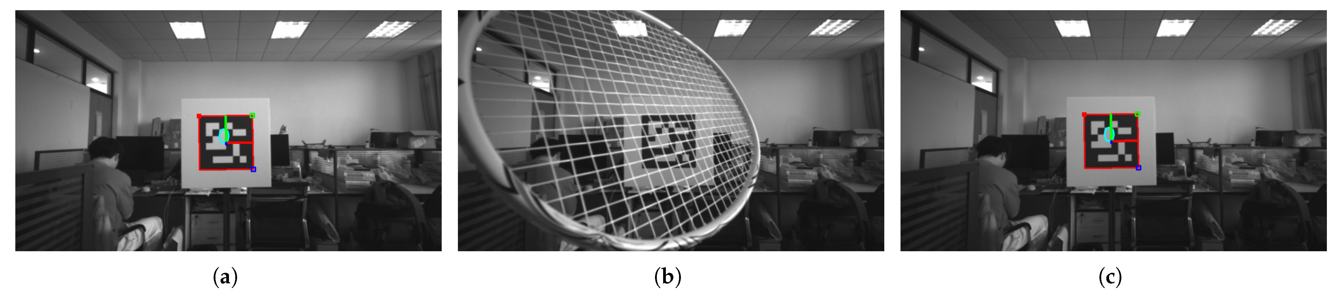
4.1. Camera Calibration

Camera calibration was used for pose estimation by transforming the object coordinates from the world frame $\mathcal{W}$ to the camera frame $\mathcal{C}$, then to the image frame $\mathcal{I}$, denoted by $O_5{X}_5{Y}_5$. To accurately determine the camera’s pose relative to the fiducial marker, it is necessary to know the intrinsic parameters of the camera, including the focal length $(f_x,f_y)$ and optical center $(c_x,c_y)$:

$$P_{\mathcal{I}}=\underset{\mathrm{Intrinsic}}{\underbrace{\left[\begin{array}{ccc}{f}_x& 0& c_x\\ 0& f_y& c_y\\ 0& 0& 1\end{array}\right]}}\underset{\mathrm{Extrinsic}}{\underbrace{[{\mathbf{R}}_{\mathcal{W}}^{\mathcal{C}}\mid {\mathbf{T}}_{\mathcal{W}}^{\mathcal{C}}]}}{P}_{\mathcal{W}}$$

(10)

where ${\mathbf{R}}_{\mathcal{W}}^{\mathcal{C}}$ is the rotation matrix, ${\mathbf{T}}_{\mathcal{W}}^{\mathcal{C}}$ is the translation vector, and $P_{\mathcal{I}}$ and $P_{\mathcal{W}}$ are points in $\mathcal{I}$ and $\mathcal{W}$, respectively.

To correct for radial and tangential distortion caused by lens imperfections, distortion coefficients must be determined; without this correction, misalignment errors can occur when the ArUco marker is far from the image center even when the camera and marker remain aligned, leading to inaccurate yaw control for the UAV.

$$\begin{array}{cc}\hfill P_d& =P_{\mathcal{I}}·(1+k_1{r}^2+k_2{r}^4+k_3{r}^6)\hfill \\ \hfill & +\left[\begin{array}{c}2q_x{q}_y\\ r^2+2q_y^2\end{array}\right]p_1+\left[\begin{array}{c}{r}^2+2q_x^2\\ 2q_x{q}_y\end{array}\right]p_2\hfill \end{array}$$

(11)

Here, $P_d$ and $P_{\mathcal{I}}$ represent the distorted and undistorted image point coordinates, respectively, while $(q_x,q_y)$ are the image point coordinates, with $r^2=q_x^2+q_y^2$ being the radial distance from the image center. The coefficients $k_1$, $k_2$, and $k_3$ describe radial distortion, while $p_1$ and $p_2$ account for tangential distortion.

The Intel RealSense D435 stereo camera mounted on the UAV was calibrated using a chessboard pattern and the Camera Calibration Toolbox in MATLAB. The calibration was performed with an image resolution of 848 × 480. The obtained intrinsic matrix $\mathbf{A}$ and distortion coefficients $(k_1,k_2,p_1,p_2,k_3)$ are shown below.

$$\mathbf{A}=\left[\begin{array}{ccc}422.27& 0& 425.83\\ 0& 422.88& 239.86\\ 0& 0& 1\end{array}\right],\left[\begin{array}{c}{k}_1\\ k_2\\ p_1\\ p_2\\ k_3\end{array}\right]=\left[\begin{array}{c}-0.0028\\ 0.0041\\ 0.00034\\ -0.00036\\ 0.000766\end{array}\right]$$

(12)

4.2. Heading Control

To adjust the UAV’s heading during autonomous landing and align the $XY$-plane of frame $\mathcal{C}$ with the $XY$-plane of frame $\mathcal{A}$, it is necessary to obtain the relative pose between $\mathcal{C}$ and $\mathcal{A}$. When the ArUco marker is detected, the relative pose ${\mathbf{r}}_{\mathrm{dev}}$ and ${\mathbf{t}}_{\mathrm{dev}}$ between $\mathcal{A}$ and $\mathcal{C}$ is obtained by the PnP algorithm [35]. Here, ${\mathbf{r}}_{\mathrm{dev}}$ is a rotation vector that describes the rotation from $\mathcal{A}$ to $\mathcal{C}$. To calculate the yaw deviation ${\psi }_{\mathrm{dev}}$ between the $O_4{Z}_4$ and $O_3{Z}_3$ axes in the $XZ$-plane of $\mathcal{C}$, we convert ${\mathbf{r}}_{\mathrm{dev}}$ into the rotation matrix ${\mathbf{R}}_{\mathcal{C}}^{\mathcal{A}}$ using Rodrigues’ formula [36]:

$${\mathbf{R}}_{\mathcal{A}}^{\mathcal{C}}={\mathbf{I}}_{3\times 3}+{\displaystyle \frac{sin∥{\mathbf{r}}_{\mathrm{dev}}∥}{∥{\mathbf{r}}_{\mathrm{dev}}∥}}{\widehat{\mathbf{r}}}_{\mathrm{dev}}+{\displaystyle \frac{1-cos∥{\mathbf{r}}_{\mathrm{dev}}∥}{{∥{\mathbf{r}}_{\mathrm{dev}}∥}^2}}{\widehat{\mathbf{r}}}_{\mathrm{dev}}^2$$

(13)

where ${\mathbf{I}}_{3\times 3}$ is the identity matrix and ${\widehat{\mathbf{r}}}_{\mathrm{dev}}$ is the skew-symmetric matrix form of ${\mathbf{r}}_{\mathrm{dev}}$. Then, ${\psi }_{\mathrm{dev}}$ can be obtained by

$${\psi }_{\mathrm{dev}}=atan2\left({\mathbf{R}}_{\mathcal{A}}^{\mathcal{C}}(1,3),{\mathbf{R}}_{\mathcal{A}}^{\mathcal{C}}(3,3)\right).$$

(14)

To determine the desired yaw angle ${\psi }_{\mathrm{des}}$, the UAV’s current yaw angle ${\psi }_{\mathrm{cur}}$ must be considered, as it is defined with respect to the world frame $\mathcal{W}$, where a yaw of zero corresponds to $X_1\in \mathcal{W}$ pointing North. Although the deviation ${\psi }_{\mathrm{dev}}$ indicates the UAV’s misalignment with the fiducial marker, it does not fully describe the UAV’s heading in $\mathcal{W}$. Therefore, both ${\psi }_{\mathrm{cur}}$ and ${\psi }_{\mathrm{dev}}$ are required to accurately compute ${\psi }_{\mathrm{des}}$, as shown in Figure 6. Because the UAV used in this study is equipped with PX4 flight controller firmware, its attitude is represented using quaternions. The following equation provides the computation of the UAV’s current yaw angle based on quaternion $\mathbf{q}=(q_0,q_1,q_2,q_3)$:

$${\psi }_{\mathrm{cur}}=atan2\left(2·\left(q_0{q}_3+q_1{q}_2\right),1-2·\left(q_2^2+q_3^2\right)\right).$$

(15)

Due to the UAV’s dynamic response lagging behind changes in ${\psi }_{\mathrm{dev}}$, directly determining ${\psi }_{\mathrm{des}}$ as ${\psi }_{\mathrm{des}}$ = ${\psi }_{\mathrm{cur}}$ + ${\psi }_{\mathrm{dev}}$ would result in an excessively large control input to the flight controller, potentially inducing oscillations in the UAV’s motion. To mitigate this issue, a PID controller is introduced, where ${\psi }_{\mathrm{dev}}$ serves as the tracking error input, generating a moderate angular correction as the control output ${\psi }_{\mathrm{out}}$; then, ${\psi }_{\mathrm{des}}$ is computed as follows:

$$\begin{array}{cc}\hfill {\psi }_{\mathrm{des}}\left(k\right)& ={\psi }_{\mathrm{cur}}\left(k\right)+K_P{\psi }_{\mathrm{dev}}\left(k\right)+K_I\Delta t\sum _{i=1}^k{\psi }_{\mathrm{dev}}\left(i\right)+K_D{\displaystyle \frac{{\psi }_{\mathrm{dev}}\left(k\right)-{\psi }_{\mathrm{dev}}(k-1)}{\Delta t}}\hfill \\ & ={\psi }_{\mathrm{cur}}\left(k\right)+{\psi }_{\mathrm{out}}\left(k\right)\hfill \end{array}$$

(16)

where $K_P$, $K_I$, and $K_D$ represent the proportional, integral, and derivative gains, respectively, and $\Delta t$ is the sampling time. In addition, to ensure stability and prevent excessive control outputs, the maximum control outputs are constrained to preset limits during each control step.

Due to the coupling between yaw and translational motions in quadrotor UAVs, simultaneous adjustment of both can cause mutual interference and reduce the efficiency of visual tracking as the UAV approaches the marker. To address this issue, an event-triggered mechanism is introduced by establishing a virtual bounding box around the UAV’s target landing point, as shown in Figure 7. When the UAV is outside the bounding box, ${\psi }_{\mathrm{des}}$ remains constant and the UAV primarily relies on translational motion to minimize position error, allowing it to quickly approach the USV. When the UAV enters the bounding box, ${\psi }_{\mathrm{des}}$ is adjusted based on ${\mathbf{r}}_{\mathrm{dev}}$. Because the position error is smaller at this stage and the translational speed decreases, the UAV can respond more swiftly to yaw control.

The target landing point is located along the $O_4{Z}_4$ axis and positioned 75 cm in front of the $O_4{X}_4{Y}_4$ plane. This ensures that the onboard camera’s FOV can fully cover the marker while maintaining a safe distance between the UAV and the marker before landing. In addition, the landing platform measures 120 × 70 cm, which enables the UAV to land near the center of the platform.

The dimensions of the bounding box were designed with reference to both the UAV’s size and its maneuvering range within the landing platform while ensuring that the fiducial marker remained within the onboard camera’s FOV, and were further refined through real-world experimental testing. To prevent the UAV from adjusting its heading angle outside of the landing platform area, the bounding box was confined within the boundaries of the platform. The UAV can be approximated as a cube with a side length of about 32 cm. Accordingly, the bounding box height was set to 60 cm, approximately twice the UAV’s body width, in order to provide sufficient vertical maneuvering space. The length and width were set to 50 cm and 25 cm, respectively. A relatively narrow width was intentionally chosen in order to reduce the influence of heading adjustments on translational motion during the UAV’s approach to the marker, thereby reducing the risk of collision with the fiducial marker. Additionally, the target landing point was positioned with distances of 15 cm and 10 cm to the front and rear planes of the bounding box, respectively. This asymmetrical placement allows the UAV to initiate heading adjustments earlier as it approaches the landing point, and ensures that if the UAV can promptly exit the bounding box and reposition itself if it gets too close to the marker.

4.3. Position Control

For vision-based position control of the UAV, the relative position ${\mathbf{t}}_{\mathrm{dev}}=[t_x,t_y,t_z]$ between the camera and the fiducial marker is utilized to generate control inputs for translational motion. In the UAV body frame $\mathcal{B}$, the position error $[e_x,e_y,e_z]$ represents the relative position between the UAV and the detected marker. Due to differences in frame definition described in Figure 1, $e_y$ and $e_z$ correspond to $t_x$ and $t_y$, respectively.

Unlike $e_y$ and $e_z$, which are directly obtained from ${\mathbf{t}}_{\mathrm{dev}}$, $e_x$ is defined as the difference between the measured forward distance obtained through the stereo vision method [37] and the desired distance $x_{\mathrm{des}}$ from the marker:

$$e_x=fB/d-x_{\mathrm{des}}$$

(17)

where f is the camera’s focal length, B is the baseline distance, and d is the disparity. In addition, to obtain the disparity of the marker center in the stereo image, the four corners of the marker are selected as feature points. The disparity for each point is calculated based on their horizontal image coordinates $\mathcal{I}\left(x\right)$ in the left and right images, denoted as ${\mathcal{I}}_{left}$ and ${\mathcal{I}}_{right}$, respectively, and the average of these four disparities is taken as the final disparity d used for distance estimation:

$$d=1/4\sum _{i=1}^4\left|{\mathcal{I}}_{left}\left(x_i\right)-{\mathcal{I}}_{right}\left(x_i\right)\right|.$$

(18)

The reason behind using stereo vision for distance estimation is to ensure more precise measurements at closer ranges to the fiducial marker. To validate this, an experiment was conducted to determine the effective detection range of the camera with respect to the ArUco marker. During the experiment, the estimated distances obtained using stereo vision and the PnP method were recorded, as shown in

Table 3. Comparison of measured distances between stereo vision, ${\mathbf{t}}_{\mathrm{dev}}\left(t_z\right)$, and ground truth.

Ground Truth (cm)	Stereo Vision (cm)	${\mathit{t}}_{\mathbf{dev}}\left({\mathit{t}}_{\mathit{z}}\right)$ (cm)
50	50	53
100	100	103
150	149	155
200	201	208
250	249	257
300	300	312
350	341	361
400	387	415
450	432	470
500	465	522
550	507	573
600	547	623
650	589	674
700	625	725
750	665	784
800	701	837
850	743	890

. The experimental results indicate that the maximum effective detection range is 850 cm. Furthermore, the Mean Absolute Error (MAE), Root Mean Square Error (RMSE), and Mean Relative Error (MRE) between the estimated distances and the ground truth were computed for both methods, with the results summarized in

Table 4. Comparison of error metrics between stereo vision and ${\mathbf{t}}_{\mathrm{dev}}\left(t_z\right)$.

Metric	Stereo Vision	${\mathit{t}}_{\mathbf{dev}}\left({\mathit{t}}_{\mathit{z}}\right)$
Mean Absolute Error	35.23 cm	18.35 cm
Root Mean Square Error	51.04 cm	21.58 cm
Mean Relative Error	5.38%	4.00%

. Over the range from 50 cm to 850 cm, the PnP method generally achieved higher overall accuracy. However, as demonstrated in Figure 8, the absolute errors between the estimated distances and the ground truth using stereo vision are lower than those of the PnP method within the range of 50 cm to 450 cm. The comparison of error metrics in

Table 5. Comparison of error metrics between stereo vision and ${\mathbf{t}}_{\mathrm{dev}}\left(t_z\right)$ (<5 m).

Metric	Stereo Vision	${\mathit{t}}_{\mathbf{dev}}\left({\mathit{t}}_{\mathit{z}}\right)$
Mean Absolute Error	4.56 cm	9.33 cm
Root Mean Square Error	8.01 cm	10.78 cm
Mean Relative Error	1.27%	3.83%

further demonstrates that stereo vision outperforms the PnP method in terms of MAE, RMSE, and MRE, indicating that stereo vision provides more precise estimates at short and medium ranges. It is worth noting that the absolute errors of the estimates obtained by stereo vision become larger than those of the PnP method when the ground truth distance exceeds 5 m. This trend can be attributed to the inherent limitations of stereo vision at longer distances, where the disparity between the left and right images becomes smaller, leading to reduced measurement precision. In contrast, ${\mathbf{t}}_{\mathrm{dev}}$, which is derived from the PnP algorithm, tends to be less accurate at close distances but demonstrates less variation in error as the distance increases, making it more reliable than stereo vision at longer ranges.

Position control of the UAV is achieved by regulating its motion along the $O_2{X}_2$, $O_2{Y}_2$, and $O_2{Z}_2$ axes of $\mathcal{B}$ using a PID controller. The controller input is the position error $[e_x,e_y,e_z]$, and the control outputs $u_x$, $u_y$, and $u_z$ can be expressed as follows:

$$\begin{array}{c}\hfill u_x\left(k\right)=K_{P_1}{e}_x\left(k\right)+K_{I_1}\Delta t\sum _{i=1}^k{e}_x\left(i\right)+K_{D_1}{\displaystyle \frac{e_x\left(k\right)-e_x(k-1)}{\Delta t}}\\ \hfill u_y\left(k\right)=K_{P_2}{e}_y\left(k\right)+K_{I_2}\Delta t\sum _{i=1}^k{e}_y\left(i\right)+K_{D_2}{\displaystyle \frac{e_y\left(k\right)-e_y(k-1)}{\Delta t}}\\ \hfill u_z\left(k\right)=K_{P_3}{e}_z\left(k\right)+K_{I_3}\Delta t\sum _{i=1}^k{e}_z\left(i\right)+K_{D_3}{\displaystyle \frac{e_z\left(k\right)-e_z(k-1)}{\Delta t}}\end{array}$$

(19)

where $K_{P_i}$, $K_{I_i}$, and $K_{D_i}$ represent the proportional, integral, and derivative gains, respectively, and $\Delta t$ represents the sampling time. In addition the maximum control outputs are constrained to preset limits during each control step in order to ensure stability and prevent excessive control outputs.

While based on the Pixhawk PX4 architecture, because the position control output $\mathbf{u}={[u_x,u_y,u_z]}^{\mathrm{T}}$ is defined in $\mathcal{B}$, the desired position ${\mathbf{p}}_{\mathrm{des}}$ of the UAV is specified in $\mathcal{W}$. Thus, a transformation is required in order to compute the UAV’s desired position in $\mathcal{W}$ at each control step. This transformation relies on the UAV’s current position ${\mathbf{p}}_{\mathrm{cur}}$, ${\psi }_{\mathrm{des}}$, and control outputs $\mathbf{u}$, formulated as follows:

$${\mathbf{p}}_{\mathrm{des}}={\mathbf{p}}_{\mathrm{cur}}+\left[\begin{array}{ccc}cos{\psi }_{\mathrm{des}}& sin{\psi }_{\mathrm{des}}& 0\\ sin{\psi }_{\mathrm{des}}& cos{\psi }_{\mathrm{des}}& 0\\ 0& 0& 1\end{array}\right]\mathbf{u}.$$

(20)

To accommodate different landing scenarios, the PID controller configuration was adjusted according to the motion state of the landing platform. In the case of a stationary platform, the integral gain in the PID controller for position control was set to zero to increase the sensitivity in compensating for position errors. However, this configuration fails to eliminate steady-state errors when tracking a moving platform, resulting in a persistent deviation from the target landing point. To overcome this limitation, the integral term was incorporated into the controller to enhance the UAV’s tracking performance in tracking a moving platform.

4.4. Failsafe Mechanism

Under clear weather conditions, the GNSS module on the UAV can receive signals from up to 28 satellites with a positioning error of around 0.7 m, as indicated by the mobile Android ground station running QGroundControl 4.4.1. However, based on observations through experiments, the accuracy of GNSS positioning generally ranges from 1 to 2 m. To ensure that the onboard camera is able to detect the fiducial marker before the UAV initiates vision-based autonomous landing, the starting position for visual guidance was set 5 m behind the GNSS position of the USV. Additionally, the initial yaw angle of the UAV was aligned with the heading of the USV.

The choice of a 5 m offset distance was based on two main considerations. First, this range lies in the middle of the effective detection distance, as shown in Table 3. Considering both the size of the two vehicles and the GNSS positioning errors, this distance ensures that the camera can detect the fiducial marker while also maintaining a relatively safe initial distance between the UAV and USV. Second, the stereo vision method provides better distance measurement accuracy compared to the PnP method within this distance, which improves the UAV’s positioning accuracy as it approaches the USV.

To provide a safeguard in cases where the fiducial marker becomes undetectable during the visual tracking phase, a failsafe mechanism is implemented to ensure operational safety. If the fiducial marker becomes undetectable for more than 0.3 s, the system automatically switches the UAV’s flight mode in the PX4 flight stack from Offboard to Hold. In Hold mode, the UAV hovers at its current position, maintaining stability against wind and other external disturbances. When the marker is detected again, the system switches the flight mode back to Offboard, allowing the UAV to resume visual tracking. To further enhance operational safety, the UAV’s onboard camera view is transmitted in real-time to the laptop ground station, allowing for continuous monitoring of the UAV’s status. If necessary, the operator can intervene and manually take control via the remote controller at any time.

To demonstrate the UAV’s response when the fiducial marker is temporarily occluded, a Hardware-In-The-Loop (HITL) simulation in Gazebo was conducted. The simulation was performed under indoor conditions, with a physical ArUco fiducial marker measuring $15\times 15$ cm placed in front of the camera. A 3D simulation environment established in Gazebo was used to run a virtual quadrotor with the same PX4 flight stack version as the physical UAV. The flight status of the simulated UAV was monitored using the QGroundControl software. Image data from the camera were processed by ROS2 control nodes, which also managed bidirectional communication with the PX4 flight controller by sending control commands and receiving state feedback. The overall simulation architecture is illustrated in Figure 9.

Figure 10 and Figure 11 the camera’s view of the fiducial marker and the UAV’s status during the simulation, including position, velocity, yaw angle, and tracking errors over time. In terms of experimental configuration, a constant positional offset was maintained between the camera and the fiducial marker, with the marker positioned at the center of the camera image and a fixed distance of 58 cm between them. Although efforts were made to align the camera’s optical axis $O_3{Z}_3$ with the marker’s normal vector $O_4{Z}_4$, a yaw angle deviation of approximately 1 degree remained, as shown in Figure 11e, which caused the UAV to compensate by consistently adjusting its yaw angle during the simulation. In addition, the target landing point was intentionally set 20 cm ahead of the marker’s center, resulting in a persistent positional error between the UAV and the target, as shown in Figure 11d. As a result, continuous motion adjustments were observed in the Gazebo simulator when the marker was detected. At the beginning of the simulation, the UAV ascended to an altitude of 10 m and hovered while waiting for visual input. At 28 s, the flight mode switched to Offboard after the visual tracking module was activated, and the UAV began moving accordingly. At 54 s, the fiducial marker was occluded manually, as shown in Figure 10b, causing the flight mode to switch from Offboard to Hold. When the marker reappeared at 75 s, the UAV automatically resumed Offboard flight mode and continued visual tracking. The simulation results indicate that the UAV is able to maintain a stable position and heading during Hold mode despite the temporary loss of marker detection. Furthermore, the flight mode can be quickly switched in response to changes in marker visibility, validating the effectiveness of the proposed failsafe mechanism in maintaining operational safety under visual uncertainty.

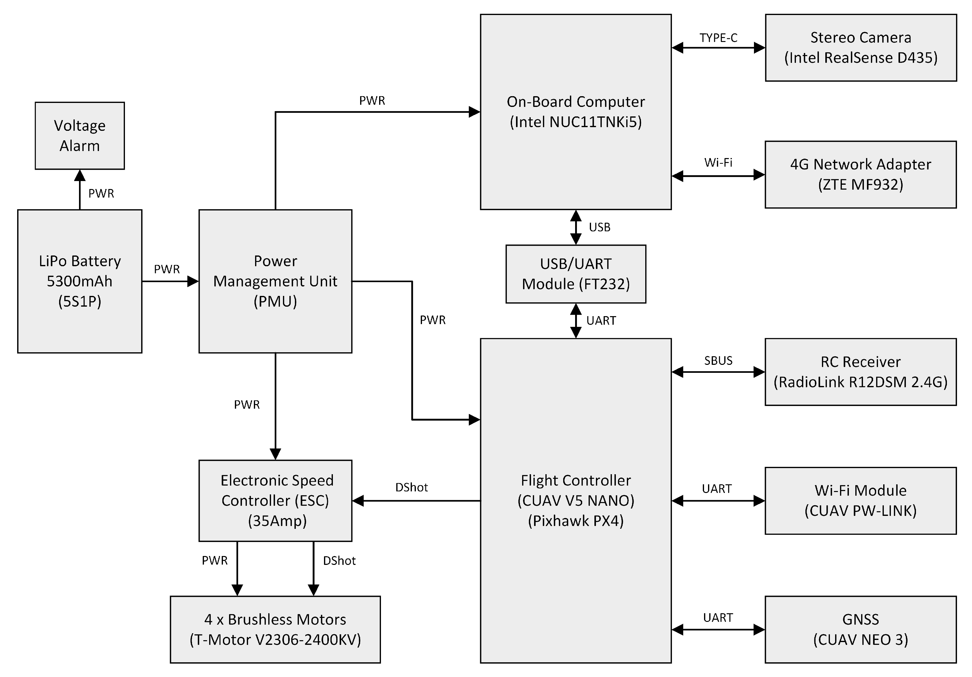
5. System Architecture

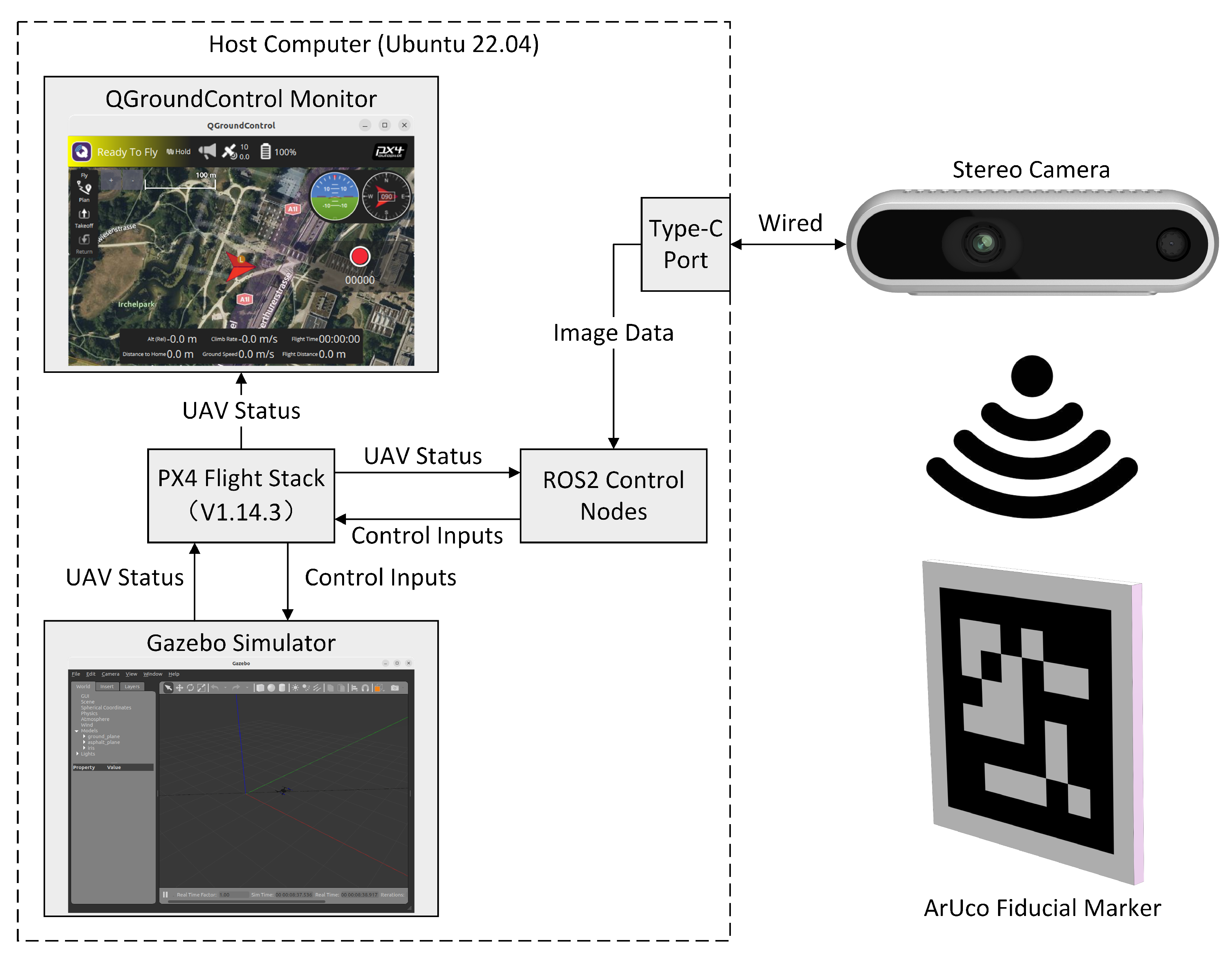
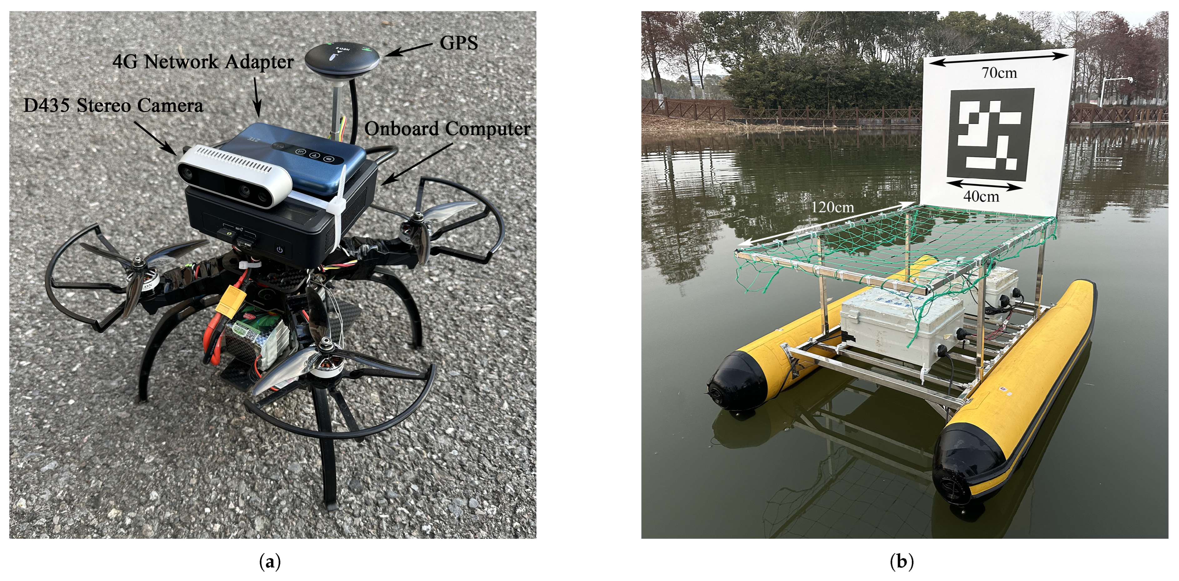
5.1. Hardware Setup

The hardware setup of the UAV is composed of four main sections: the computational unit, power unit, communication devices, and sensors, as depicted in Figure 12. The computational unit consists of an onboard computer and a Pixhawk flight controller. The onboard computer is used for processing data received from sensors, maintaining the network connection, and transmitting commands to the flight controller. The flight controller processes these commands and generates D-shot signals for the electronic speed controllers, ensuring precise motor operation. The power unit of the UAV is comprised of a Lithium Polymer (LiPo) battery, a Power Management Unit (PMU), Electronic Speed Controllers (ESCs), and motors. The onboard computer and ESCs are directly powered by the LiPo battery, while the Pixhawk flight controller is powered through the PMU. The sensors primarily comprise a D435 stereo camera, a GNSS unit, an Inertial Measurement Unit (IMU), an electronic compass, and a barometer. For communication, the UAV is equipped with a WiFi module and a 4G network adapter. The WiFi module enables short-range communication with the Android ground station using QGroundControl, while the 4G adapter provides connectivity to the public internet, facilitating long-range data transmission and reception between the UAV and the laptop ground station. To implement this setup, a custom-built quadcopter was developed featuring a 250 mm wheelbase and a total weight of 1.8 kg, as shown in Figure 13a. Carbon fiber plates were specifically designed to securely mount the Li-Po battery, flight controller, GPS, and onboard computer. The Infra-Red (IR) projector on the D435 camera is covered to prevent laser dots from impacting the ArUco marker, which could interfere with the marker detection.

Similar to the UAV, the hardware architecture of the USV also consists of four main sections, as shown in Figure 14. The key difference is that its computational unit only includes an onboard computer, which computes Pulse-Width Modulation (PWM) duty cycle commands. These commands are sent to PWM signal generators, which produce PWM signals and deliver them to the ESCs to control the motors. The USV is equipped with a UAV landing platform that includes a vertically placed ArUco marker board. The dimensions of the board are $70\times 70$ cm, with the ArUco marker itself measuring 40 × 40 cm. The horizontal landing area measures $70\times 120$ cm, with a nylon net positioned at the center of the landing zone to capture the UAV. The design of the surface vehicle and landing platform is illustrated in Figure 13b.

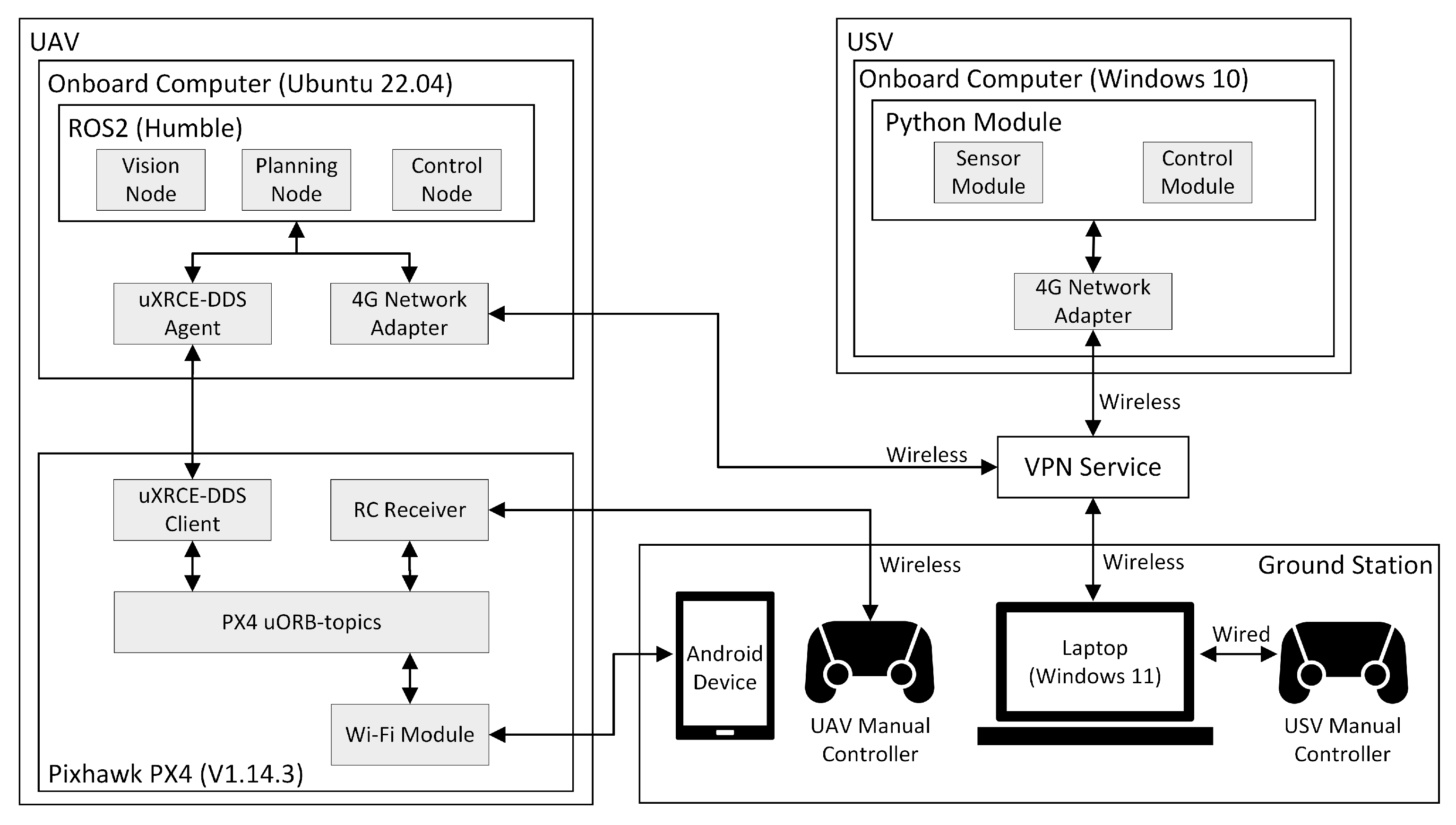
5.2. System Communication

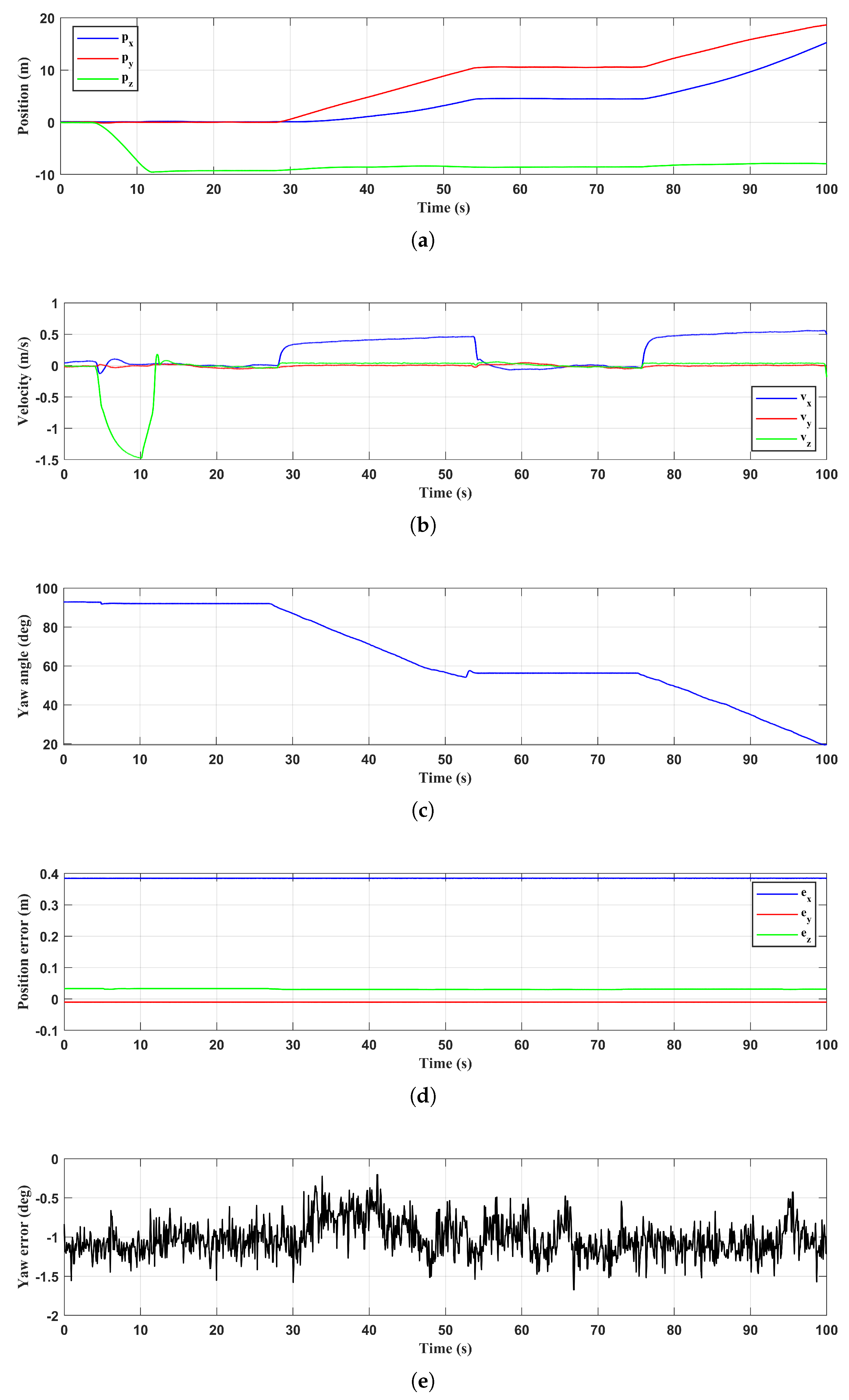
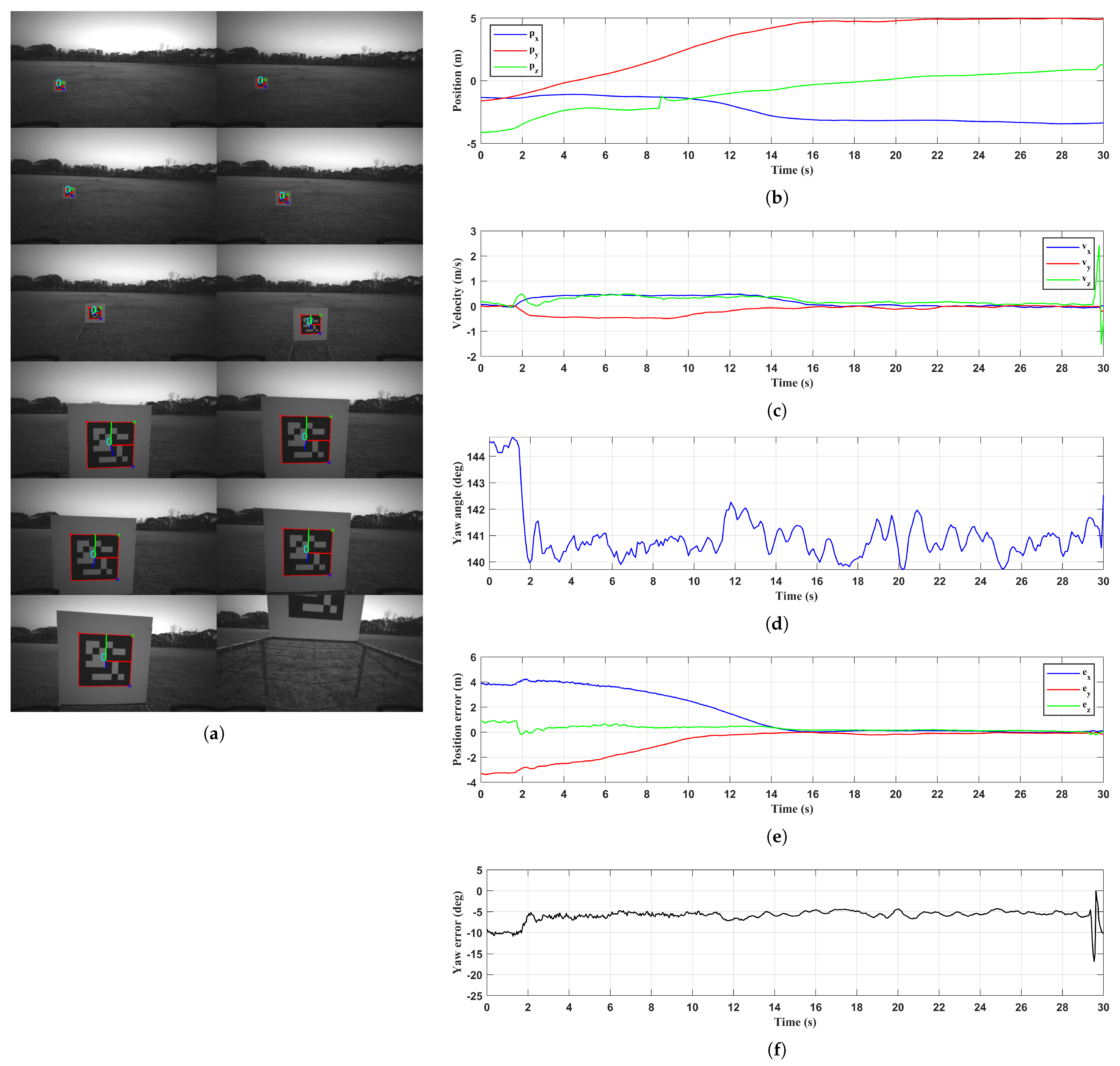
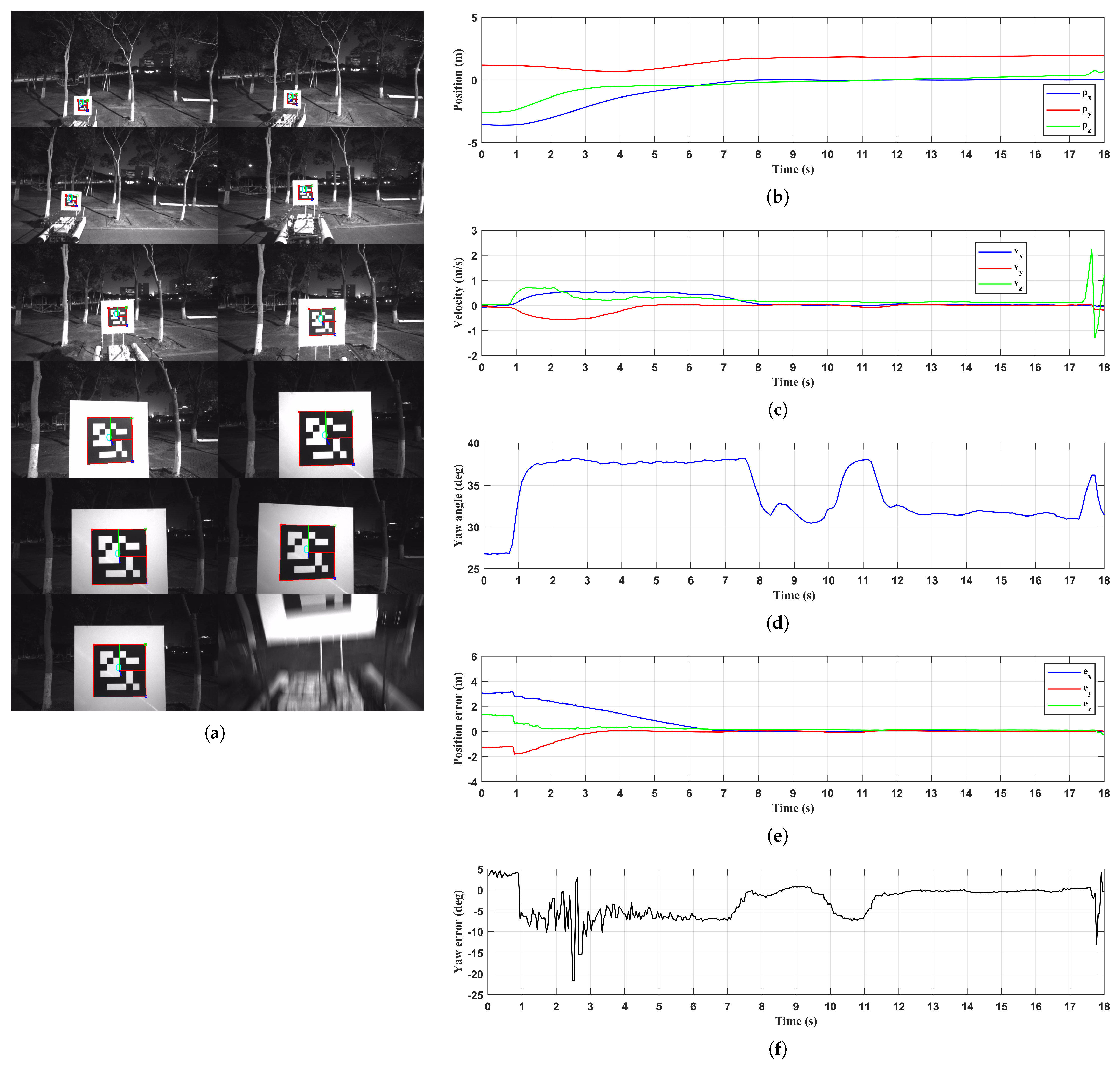
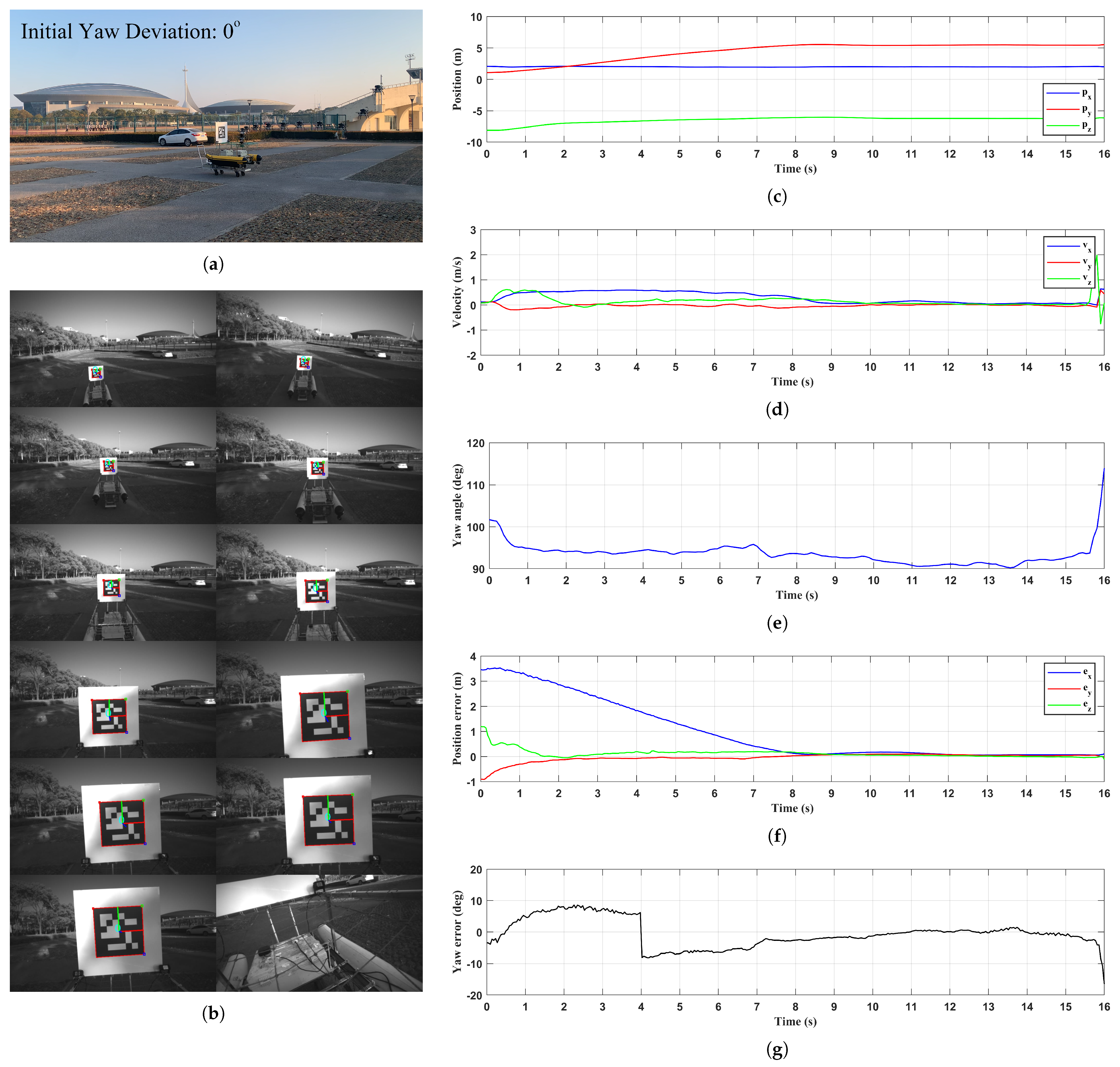
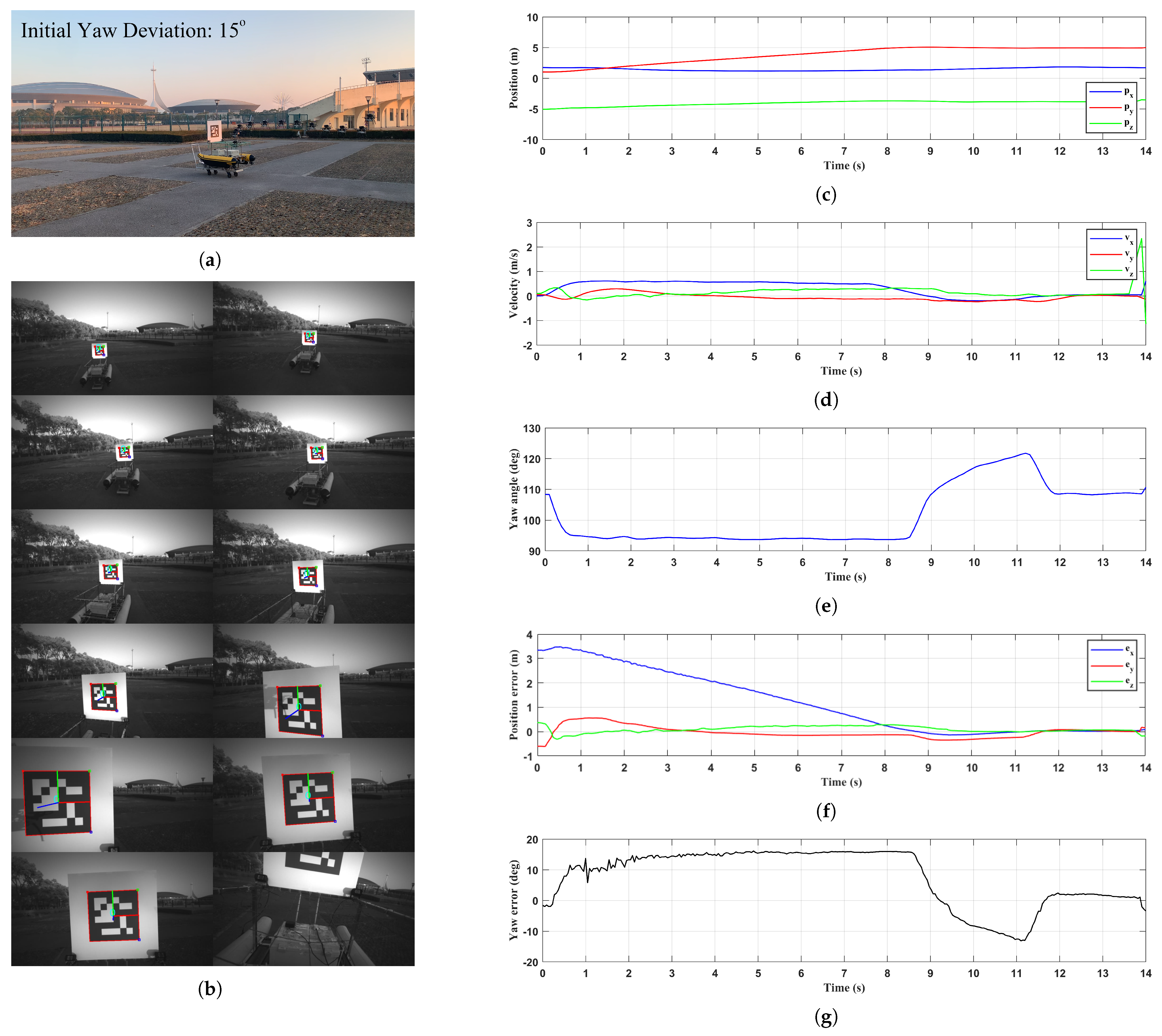
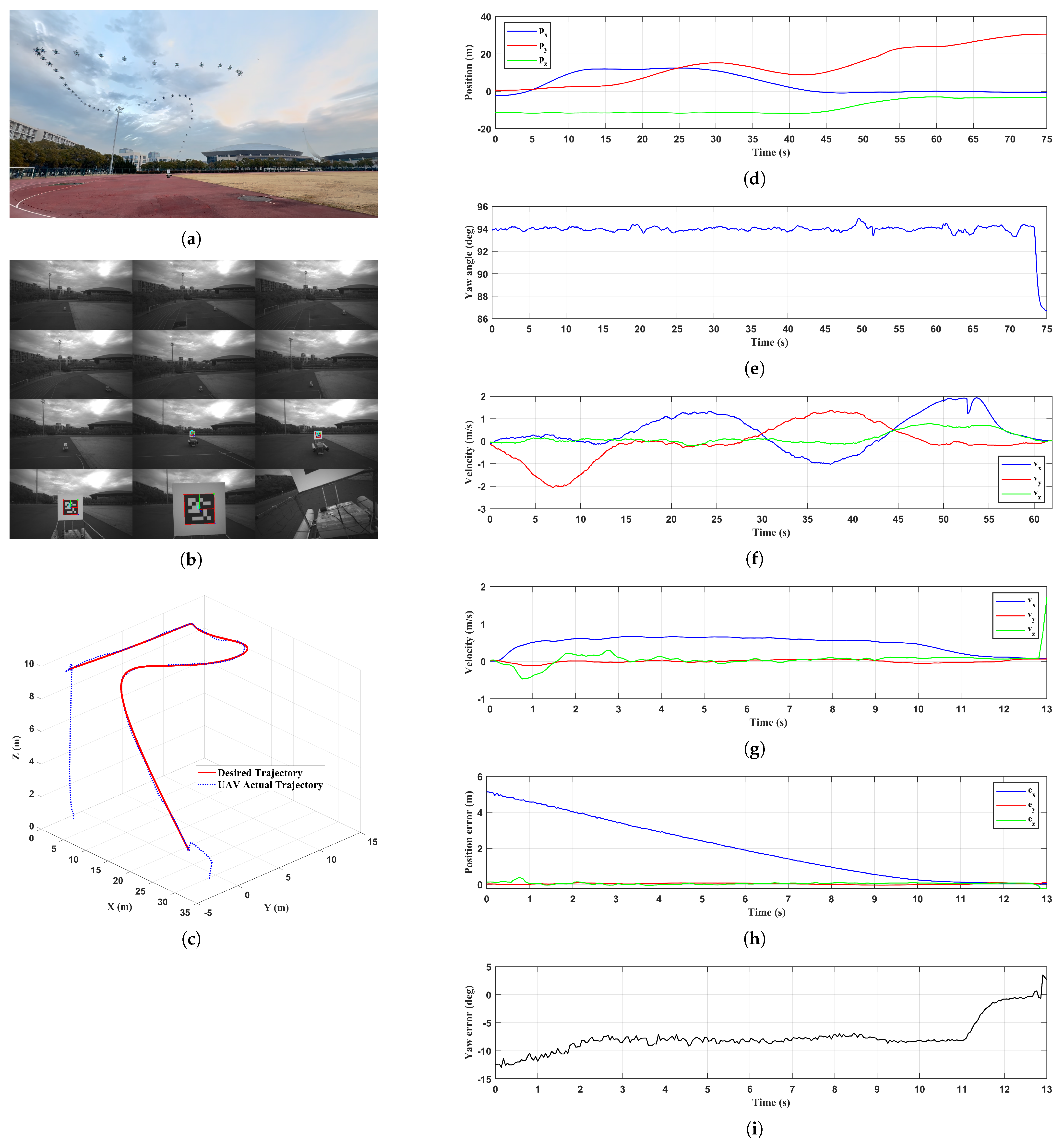
The communication architecture consists of three main components: the UAV, the USV, and the ground station, as shown in Figure 15. The UAV and USV are equipped with 4G network adapters, enabling communication with the laptop ground station through a VPN connection. This setup allows the operator to remotely access the UAV’s ROS2 system and the lower computer on the USV.

The ground station includes controllers for manual control. The UAV manual controller is used for intervention in emergency situations, connecting to the UAV’s RC receiver for direct control. The USV manual controller is connected to the laptop, which hosts the upper computer interface for the USV. This interface is responsible for configuring control modes such as manual control or autonomous course keeping as well as for visualizing data transmitted from the USV through the VPN, including sensor measurements, PWM duty cycles, and mapping information. Additionally, control signals generated within the upper computer interface are transmitted to the USV’s lower computer through the VPN, enabling bidirectional communication and control of the USV.

The UAV’s onboard computer operates on Ubuntu 22.04 with ROS2 Humble. ROS2 packages are developed for visual detection, minimum snap trajectory planning, and offboard flight control of the UAV. The USV’s onboard computer operates on Windows 10 and executes the lower computer program developed in Python 3.10.12. This program primarily handles sensor data processing and implements a PD controller for USV control.

Communication between the UAV flight controller and the onboard computer is managed by the uXRCE-DDS middleware V2.4.3. The UAV flight control firmware used in this study is Pixhawk PX4 V1.14.3, released on 25 May 2024. Starting from version V1.14.0, the PX4 firmware integrates uXRCE-DDS middleware to replace the FastRTPS middleware. In this system, the onboard computer runs the uXRCE-DDS agent, while the flight controller runs the uXRCE-DDS client. The middleware facilitates the publication and subscription of internal uORB messages within the flight controller through the Data Distribution Service (DDS), enabling communication with the onboard computer running ROS2 [38,39].

6. Experiments

6.1. Stationary Platform

The experiments in this section evaluate the effect of the event-triggered mechanism on visual guidance with a stationary platform as well as the tracking performance under different initial angular deviations between the UAV and the fiducial marker. Additionally, the UAV’s ability to track the improved minimum snap trajectory for approaching the USV and to perform landing based on visual guidance is evaluated.

6.1.1. Event-Triggered Mechanism Validation

This subsection validates the impact of the event-triggered mechanism on the UAV’s autonomous landing process based on visual guidance through two sets of comparative experiments. The results of the experiments conducted without and with the event-triggered mechanism are presented in Figure 16 and Figure 17, respectively. The experimental results include the onboard camera view during the landing process, the UAV’s position and yaw angle in the world frame $\mathcal{W}$, the velocity in the body frame $\mathcal{B}$, the position error between the onboard camera and the target landing point, and the yaw angle error between the onboard camera and the fiducial marker.

It should be noted that the world frame $\mathcal{W}$ is defined at the UAV’s position at the moment of power-up rather than at the location where the vehicle is armed for takeoff. As a result, the origin of $\mathcal{W}$ remains fixed throughout the experiments regardless of the UAV’s actual takeoff position. Additionally, due to inherent sensor measurement errors, the estimated position of the UAV in $\mathcal{W}$ may deviate from its physical location in the real world. These factors explain the discrepancies observed in Figure 16b, where the UAV appears to start from a non-zero horizontal offset and an altitude higher than its actual height above the ground.

In both sets of experiments, the UAV was positioned at a similar starting point, with the fiducial marker located to the lower left of the onboard camera view. Additionally, to ensure a broader coverage of lighting conditions, the experiment in Figure 16 was conducted under favorable daytime lighting, while the one in Figure 17 was conducted at night under artificial illumination from street lamps. The experimental results show that although the UAV was able to complete the autonomous landing in the absence of the event-triggered mechanism, it consistently failed to correct the angular offset with respect to the fiducial marker, demonstrating limited capability in heading adjustment. In contrast, with the event-triggered mechanism enabled, the landing duration was significantly reduced from 30 s to 18 s. As shown in Figure 17e,f, the UAV not only approached the target landing point more efficiently but also adjusted its heading more promptly and accurately with respect to the marker. These results demonstrate that the event-triggered mechanism contributes to more efficient autonomous landing during the visual guidance stage and enhances the UAV’s heading control capabilities.

It should also be noted that the UAV’s velocity along the z-axis in the body frame $\mathcal{B}$ exhibits sudden fluctuations in Figure 16c and Figure 17c, occurring near 30 s and 18 s, respectively. These fluctuations result from the shutdown of the motors after the UAV reached the target landing point, causing the UAV to drop onto the platform and resulting in a transient oscillation in its vertical velocity.

6.1.2. Yaw Deviation Adjustment

In real-world environments, external disturbances and instability in the motions of the UAV and USV can cause a yaw angle deviation between the onboard camera and the fiducial marker as the UAV approaches the USV. To evaluate whether the UAV can successfully correct such a deviation and complete the landing process, two sets of comparative experiments were conducted. Figure 18 and Figure 19 respectively present the experimental results for two scenarios with relatively small and relatively large initial deviations between the UAV and the USV. The results include the third-person ground view, the onboard camera view, the UAV’s position and yaw angle in the world frame $\mathcal{W}$, the velocity in the body frame $\mathcal{B}$, the position error between the onboard camera and the target landing point, and the yaw angle error between the onboard camera and the fiducial marker.

In both experiments, the UAV was positioned at a similar starting point, with the fiducial marker located below the center of the onboard camera view. In Figure 18, the initial yaw angle offset between the UAV and the USV was set to $0^{\circ }$, whereas in Figure 19 it was set to ${15}^{\circ }$. The experimental results show that the UAV successfully completed the autonomous landing in both cases. With the assistance of the event-triggered mechanism, the yaw angle deviation between the onboard camera and the fiducial marker was corrected to nearly $0^{\circ }$ before landing. As shown in Figure 19e, the UAV corrected the yaw angle deviation from ${15}^{\circ }$ to nearly $0^{\circ }$ within approximately 3 s through only two adjustment actions and maintained stable alignment thereafter, demonstrating that the proposed method can effectively handle heading and position adjustments under certain initial yaw deviations. It should be noted that in Figure 18g a sudden change in the yaw angle error can be observed around 4 s. This was caused by a brief oscillation of the UAV during the landing process, leading to a step change in the yaw angle calculation. However, no corresponding change is observed in Figure 18e at the same time, as the UAV had not yet entered the bounding box, meaning that the detected yaw angle deviation did not trigger any heading adjustment. This also demonstrates that the bounding box size adopted in this study is suitable for real-world applications.

6.1.3. Approaching and Landing

To evaluate the tracking performance of the improved minimum snap trajectory and visual guidance with the event-triggered mechanism, an experiment was conducted in a ground-based scenario with a wind speed of 12 km/h. In the experiment, the UAV first ascended to an altitude of 10 m. A target flight trajectory was then generated based on GNSS waypoints and the improved minimum snap trajectory generation algorithm, with the starting point set at the UAV’s current position and the endpoint located 5 m behind the USV’s GNSS position. The intermediate waypoints were automatically generated by proportionally scaling the waypoints selected in Figure 5b. Figure 20 presents the experimental results, including the third-person ground view, the onboard camera view, the comparison between the desired trajectory and the actual flight trajectory, the UAV’s position and yaw angle in the world frame $\mathcal{W}$, the velocity in the body frame $\mathcal{B}$ during the Approaching and Landing stages, the position error between the onboard camera and the target landing point, and the yaw angle error between the onboard camera and the fiducial marker.

The experimental results show that the UAV completed the autonomous landing in 75 s, with the Approaching stage lasting 62 s and the Landing stage lasting 13 s. During the Approaching stage, as illustrated in Figure 20c, the deviation between the actual flight trajectory and the desired trajectory remained small, with a maximum deviation of 0.6 m. Moreover, as shown in Figure 20f, although the UAV’s velocity exhibited slight fluctuations, the overall velocity remained smooth, indicating that the UAV maintained stable flight performance throughout the process. Figure 20g–i presents the experimental results of the Landing stage based on visual guidance. It can be observed that the initial positional offset between the UAV and the USV was approximately 5 m, which is close to the system design. Additionally, there was an initial yaw angle deviation of approximately ${10}^{\circ }$ between the onboard camera and the fiducial marker. As the UAV maintained an average forward velocity of 0.6 m/s, it successfully entered the bounding box and completed the heading adjustment within 2 s, reducing the yaw angle deviation to $0^{\circ }$ and achieving autonomous landing.

In summary, the experimental results demonstrate that the proposed method which divides the autonomous landing process into the Approaching and Landing stages can effectively achieve autonomous UAV landing on a small USV while overcoming the limited perception range of the visual system.

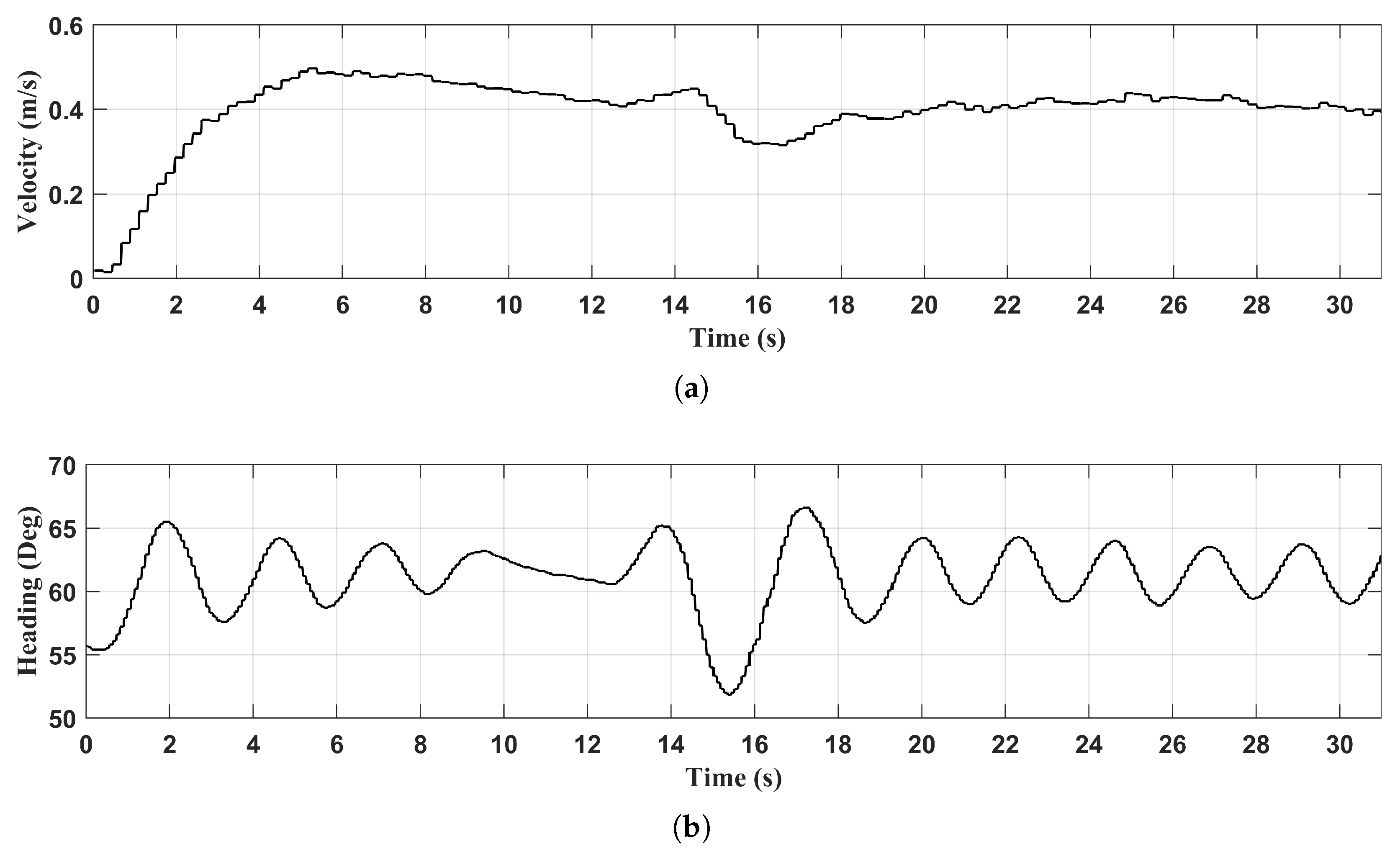
6.2. Moving Platform

Building on the successful implementation of autonomous landing on a stationary platform, this section further evaluates the UAV’s capability to perform vision-based autonomous landing on a moving platform in both terrestrial and river environments.

6.2.1. Terrestrial Environment

In this experiment, the USV was mounted on a movable cart and manually pulled at a constant speed of 0.2 m/s, simulating a scenario where the USV moves along a fixed heading. The UAV was initially positioned approximately 3 m away from the fiducial marker, with the marker located below the center of the onboard camera view. Figure 21 presents the experimental results, including the third-person ground view, the onboard camera view, the UAV’s position and yaw angle in the world frame $\mathcal{W}$, the velocity in the body frame $\mathcal{B}$, the position error between the onboard camera and the target landing point, and the yaw angle error between the onboard camera and the fiducial marker.

The experimental results show that the UAV maintained a stable forward velocity of approximately 0.6 m/s and completed the entire process within 15 s. Compared to the stationary platform experiments, although the distance between the UAV and the target landing point continuously decreased, the duration of the process became longer, as illustrated in Figure 21f. Additionally, the vibration of the fiducial marker caused by the cart movement led the UAV to exhibit more noticeable fluctuations in the yaw angle error when adjusting its position. However, as shown in Figure 21g, these fluctuations remained minor, with an average deviation of less than $2^{\circ }$. It should also be noted that near 15 s in Figure 21e a sudden change in the UAV’s heading can be observed, which was caused by a brief oscillation of the UAV after touchdown. These results verify the effectiveness of the proposed method for UAV autonomous landing on a moving platform, providing a solid foundation for the subsequent experiment conducted in the river environment.

6.2.2. River Environment

In this experiment, the USV was deployed on a river to perform autonomous course keeping at an average forward speed of 0.4 m/s. The UAV was initially positioned approximately 3 m away from the fiducial marker, with the marker located at the center of the onboard camera view. Figure 22 presents the UAV experimental results, including the third-person ground view, the onboard camera view, the UAV’s position and yaw angle in the world frame $\mathcal{W}$, the velocity in the body frame $\mathcal{B}$, the position error between the onboard camera and the target landing point, and the yaw angle error between the onboard camera and the fiducial marker. In addition, Figure 23 presents the USV experimental results, including the forward velocity and heading.

During the experiment, external disturbances such as wind and waves were minimal, resulting in negligible pitch and roll motions of the USV. By utilizing the heading information provided by the electronic compass, a PD controller was implemented on the USV to drive the thrusters for autonomous course-keeping. The controller parameters were tuned through a trial-and-error approach to achieve stable forward speed and heading during navigation. However, as shown in Figure 23b, the USV exhibited yaw oscillations due to the limitations of the parameter setting of the PD controller and the dynamic characteristics of the USV, with the heading angle initially fluctuating between ${55}^{\circ }$ and ${65}^{\circ }$ before gradually narrowing to a range between ${59}^{\circ }$ and ${64}^{\circ }$. Although the yaw angle error ${\psi }_{\mathrm{dev}}$ experienced noticeable oscillations during the period from 0 to 16 s in Figure 22g due to the USV’s motion, the UAV’s heading angle remained near ${60}^{\circ }$, aligned with the USV’s desired heading. This stability was because the UAV was still outside the bounding box during the initial phase of visual tracking. After entering the bounding box at 29 s, the UAV promptly adjusted its heading, reducing the yaw angle error within 1.5 s, then completed the landing successfully.

It is worth noting that during the period from 7 to 15 s in Figure 22f, the relative distance between the UAV and the USV remained steady at approximately 2.2 m. However, because the visual tracking controller incorporated an integral gain, this steady-state error was subsequently corrected as the UAV continued to track the USV.

To conclude, these results demonstrate that the UAV was able to maintain stable tracking performance based on visual guidance despite the presence of minor yaw oscillations from the USV. Integration of the integral term in the controller effectively corrected the steady-state errors, enabling the UAV to steadily approach the USV and complete the autonomous landing in a river environment.

7. Conclusions

This paper introduces an improved minimum snap trajectory planning algorithm integrated with vision-based guidance for autonomous landing of a UAV on a small-sized USV. Compared to other trajectory generation algorithms discussed in this paper, the proposed algorithm can generate smoother trajectories while ensuring that the trajectory passes through all designated waypoints with reduced deviation from the target flight path. Furthermore, to improve the tracking performance of vertically positioned fiducial marker, an event-triggered mechanism is introduced based on a virtual bounding box around the UAV’s target landing point. This method effectively decouples the UAV’s translational motion from its yaw control, reducing the adjustment time during the visual tracking process. To validate the proposed method, system consisting of a quadrotor UAV and a USV equipped with a landing platform was developed for the experimental setup. Experiments were carried out in both terrestrial and river environments. The UAV successfully conducted autonomous landings on both stationary and moving platforms, demonstrating the effectiveness and practicality of the proposed approach. The video recordings of the experiments are provided in Appendix A.

Future research will explore a more integrated approach towards autonomous landing of UAVs on USVs in river environments, focusing on vision-based coordination between the UAV and USV. By incorporating USV motion control into the landing process, we aim to enhance landing efficiency and adaptability in dynamic conditions.

References

1. Yang, X.; Zhao, J.; Zhao, L.; Zhang, H.; Li, L.; Ji, Z.; Ganchev, I. Detection of River Floating Garbage Based on Improved YOLOv5. Mathematics 2022, 10, 4366. [Google Scholar] [CrossRef]
2. Liao, Y.-H.; Juang, J.-G. Real-Time UAV Trash Monitoring System. Appl. Sci. 2022, 12, 1838. [Google Scholar] [CrossRef]
3. Duan, H.; Liu, S. Unmanned Air/Ground Vehicles Heterogeneous Cooperative Techniques: Current Status and Prospects. Sci. China Technol. Sci. 2010, 53, 1349–1355. [Google Scholar] [CrossRef]
4. Grlj, C.G.; Krznar, N.; Pranjić, M. A Decade of UAV Docking Stations: A Brief Overview of Mobile and Fixed Landing Platforms. Drones 2022, 6, 17. [Google Scholar] [CrossRef]
5. Li, J.; Zhang, G.; Jiang, C.; Zhang, W. A Survey of Maritime Unmanned Search System: Theory, Applications and Future Directions. Ocean. Eng. 2023, 285, 115359. [Google Scholar] [CrossRef]
6. Specht, M. Methodology for Performing Bathymetric and Photogrammetric Measurements Using UAV and USV Vehicles in the Coastal Zone. Remote Sens. 2024, 16, 3328. [Google Scholar] [CrossRef]
7. Usama, A.; Dora, M.; Elhadidy, M.; Khater, H.; Alkelany, O. First Person View Drone-FPV. In The International Undergraduate Research Conference; The Military Technical College: Cairo, Egypt, 2021; Volume 5, pp. 437–440. [Google Scholar]
8. Wilson, A.; Kumar, A.; Jha, A.; Cenkeramaddi, L.R. Embedded Sensors, Communication Technologies, Computing Platforms and Machine Learning for UAVs: A Review. IEEE Sens. J. 2021, 22, 1807–1826. [Google Scholar] [CrossRef]
9. Zeng, Q.; Jin, Y.; Yu, H.; You, X. A UAV Localization System Based on Double UWB Tags and IMU for Landing Platform. IEEE Sens. J. 2023, 23, 10100–10108. [Google Scholar] [CrossRef]
10. Ochoa-de Eribe-Landaberea, A.; Zamora-Cadenas, L.; Peñagaricano-Muñoa, O.; Velez, I. UWB and IMU-Based UAV’s Assistance System for Autonomous Landing on a Platform. Sensors 2022, 22, 2347. [Google Scholar] [CrossRef]
11. Gyagenda, N.; Hatilima, J.V.; Roth, H.; Zhmud, V. A Review of GNSS-Independent UAV Navigation Techniques. Robot. Auton. Syst. 2022, 152, 104069. [Google Scholar] [CrossRef]
12. Yang, Y.; Xiong, X.; Yan, Y. UAV Formation Trajectory Planning Algorithms: A Review. Drones 2023, 7, 62. [Google Scholar] [CrossRef]
13. Demiane, F.; Sharafeddine, S.; Farhat, O. An Optimized UAV Trajectory Planning for Localization in Disaster Scenarios. Comput. Netw. 2020, 179, 107378. [Google Scholar] [CrossRef]
14. Shao, G.; Ma, Y.; Malekian, R.; Yan, X.; Li, Z. A Novel Cooperative Platform Design for Coupled USV–UAV Systems. IEEE Trans. Ind. Inform. 2019, 15, 4913–4922. [Google Scholar] [CrossRef]
15. Ji, J.; Yang, T.; Xu, C.; Gao, F. Real-Time Trajectory Planning for Aerial Perching. In Proceedings of the 2022 IEEE/RSJ International Conference on Intelligent Robots and Systems (IROS), Kyoto, Japan, 23–27 October 2022; pp. 10516–10522. [Google Scholar]
16. Gao, Y.; Ji, J.; Wang, Q.; Jin, R.; Lin, Y.; Shang, Z.; Cao, Y.; Shen, S.; Xu, C.; Gao, F. Adaptive Tracking and Perching for Quadrotor in Dynamic Scenarios. IEEE Trans. Robot. 2023, 40, 499–519. [Google Scholar] [CrossRef]
17. Xin, L.; Tang, Z.; Gai, W.; Liu, H. Vision-Based Autonomous Landing for the UAV: A Review. Aerospace 2022, 9, 634. [Google Scholar] [CrossRef]
18. Polvara, R.; Sharma, S.; Wan, J.; Manning, A.; Sutton, R. Vision-Based Autonomous Landing of a Quadrotor on the Perturbed Deck of an Unmanned Surface Vehicle. Drones 2018, 2, 15. [Google Scholar] [CrossRef]
19. Park, Y.; Park, C.; Song, W.; Lee, C.; Kwon, J.; Park, J.; Noh, G.; Lee, D. Fiducial Marker-Based Autonomous Landing Using Image Filter and Kalman Filter. Int. J. Aeronaut. Space Sci. 2024, 25, 190–199. [Google Scholar] [CrossRef]
20. Krogius, M.; Haggenmiller, A.; Olson, E. Flexible Layouts for Fiducial Tags. In Proceedings of the 2019 IEEE/RSJ International Conference on Intelligent Robots and Systems (IROS), Macau, China, 3–8 November 2019; pp. 1898–1903. [Google Scholar]
21. Xu, Z.-C.; Hu, B.-B.; Liu, B.; Wang, X.; Zhang, H.-T. Vision-Based Autonomous Landing of Unmanned Aerial Vehicle on a Motional Unmanned Surface Vessel. In Proceedings of the 2020 39th Chinese Control Conference (CCC), Shenyang, China, 27–29 July 2020; pp. 6845–6850. [Google Scholar]
22. Nguyen, T.-M.; Nguyen, T.H.; Cao, M.; Qiu, Z.; Xie, L. Integrated Uwb-Vision Approach for Autonomous Docking of Uavs in Gps-Denied Environments. In Proceedings of the 2019 International Conference on Robotics and Automation (ICRA), Montreal, QC, Canada, 20–24 May 2019; pp. 9603–9609. [Google Scholar]
23. Procházka, O.; Novák, F.; Báča, T.; Gupta, P.M.; Pěnička, R.; Saska, M. Model Predictive Control-Based Trajectory Generation for Agile Landing of Unmanned Aerial Vehicle on a Moving Boat. Ocean. Eng. 2024, 313, 119164. [Google Scholar] [CrossRef]
24. Mellinger, D.; Kumar, V. Minimum Snap Trajectory Generation and Control for Quadrotors. In Proceedings of the 2011 IEEE International Conference on Robotics and Automation, Shanghai, China, 9–13 May 2011; pp. 2520–2525. [Google Scholar]
25. Lee, T.; Leok, M.; McClamroch, N.H. Geometric Tracking Control of a Quadrotor UAV on SE (3). In Proceedings of the 49th IEEE Conference on Decision and Control (CDC), Atlanta, GA, USA, 15–17 December 2010; pp. 5420–5425. [Google Scholar]
26. Stellato, B.; Banjac, G.; Goulart, P.; Bemporad, A.; Boyd, S. OSQP: An Operator Splitting Solver for Quadratic Programs. Math. Program. Comput. 2020, 12, 637–672. [Google Scholar] [CrossRef]
27. Lian, L.; Zong, X.; He, K.; Yang, Z. Trajectory Optimization of Unmanned Surface Vehicle Based on Improved Minimum Snap. Ocean. Eng. 2024, 302, 117719. [Google Scholar] [CrossRef]
28. Tayebi Arasteh, S.; Kalisz, A. Conversion between Cubic Bezier Curves and Catmull–Rom Splines. SN Comput. Sci. 2021, 2, 398. [Google Scholar] [CrossRef]
29. Thibbotuwawa, A.; Nielsen, P.; Zbigniew, B.; Bocewicz, G. Energy Consumption in Unmanned Aerial Vehicles: A Review of Energy Consumption Models and Their Relation to the UAV Routing. In Information Systems Architecture and Technology: Proceedings of 39th International Conference on Information Systems Architecture and Technology–ISAT 2018: Part II; Springer: Berlin/Heidelberg, Germany, 2019; pp. 173–184. [Google Scholar]
30. Abeywickrama, H.V.; Jayawickrama, B.A.; He, Y.; Dutkiewicz, E. Comprehensive Energy Consumption Model for Unmanned Aerial Vehicles, Based on Empirical Studies of Battery Performance. IEEE Access 2018, 6, 58383–58394. [Google Scholar] [CrossRef]
31. Garrido-Jurado, S.; Munoz-Salinas, R.; Madrid-Cuevas, F.J.; Marin-Jimenez, M.J. Automatic Generation and Detection of Highly Reliable Fiducial Markers under Occlusion. Pattern Recognit. 2014, 47, 2280–2292. [Google Scholar] [CrossRef]
32. Garrido-Jurado, S.; Munoz-Salinas, R.; Madrid-Cuevas, F.J.; Medina-Carnicer, R. Generation of Fiducial Marker Dictionaries Using Mixed Integer Linear Programming. Pattern Recognit. 2016, 51, 481–491. [Google Scholar] [CrossRef]
33. Romero-Ramirez, F.J.; Munoz-Salinas, R.; Medina-Carnicer, R. Speeded up Detection of Squared Fiducial Markers. Image Vis. Comput. 2018, 76, 38–47. [Google Scholar] [CrossRef]
34. Aruco Nano 4 Release. Available online: https://www.youtube.com/watch?v=U3sfuy88phA (accessed on 22 December 2022).
35. Marchand, E.; Uchiyama, H.; Spindler, F. Pose Estimation for Augmented Reality: A Hands-on Survey. IEEE Trans. Vis. Comput. Graph. 2015, 22, 2633–2651. [Google Scholar] [CrossRef] [PubMed]
36. Dai, J.S. Euler–Rodrigues Formula Variations, Quaternion Conjugation and Intrinsic Connections. Mech. Mach. Theory 2015, 92, 144–152. [Google Scholar] [CrossRef]
37. O’Riordan, A.; Newe, T.; Dooly, G.; Toal, D. Stereo Vision Sensing: Review of Existing Systems. In Proceedings of the 2018 12th International Conference on Sensing Technology (ICST), Limerick, Ireland, 4–6 December 2018; pp. 178–184. [Google Scholar]
38. Macenski, S.; Foote, T.; Gerkey, B.; Lalancette, C.; Woodall, W. Robot Operating System 2: Design, Architecture, and Uses in the Wild. Sci. Robot. 2022, 7, eabm6074. [Google Scholar] [CrossRef]
39. Macenski, S.; Soragna, A.; Carroll, M.; Ge, Z. Impact of ROS 2 Node Composition in Robotic Systems. IEEE Robot. Auton. Lett. (RA-L) 2023, 8, 3996–4003. [Google Scholar] [CrossRef]
Figure 1. Definition of coordinate frames for the proposed system and labeling of UAV arms.
Drones 09 00364 g001
Figure 2. Generated trajectories based on minimum snap (T = 180 s).
Drones 09 00364 g002
Figure 3. Generated trajectories based on minimum snap by different time allocations: (a) T = 700 s, (b) T = 1000 s.
Drones 09 00364 g003
Figure 4. Generated trajectory based on improved minimum snap algorithm (T = 180 s).
Drones 09 00364 g004
Figure 5. Different trajectory generation algorithms used for comparison: (a) minimum snap trajectory; (b) improved minimum snap trajectory; (c) minimum snap trajectory with corridor constraint; (d) trajectory based on Bézier curves with Catmull–Rom spline.
Drones 09 00364 g005
Figure 6. Illustration of yaw control in the world frame.
Drones 09 00364 g006
Figure 7. Illustration of bounding box and UAV’s translational movement.
Drones 09 00364 g007
Figure 8. Comparison of the absolute error for the stereo vision and PnP methods with respect to the ground truth.
Drones 09 00364 g008
Figure 9. System architecture for the HITL simulation using Gazebo and PX4 flight stack.
Drones 09 00364 g009
Figure 10. UAV camera view of the fiducial marker: (a) initialize Offboard flight mode when the marker is detected, (b) switch to Hold flight mode when the marker is occluded, (c) switch back to Offboard flight mode after the marker is re-detected.
Drones 09 00364 g010
Figure 11. UAV fail−safe response to fiducial marker occlusion: (a) UAV position in the world frame W , (b) UAV velocity in the body frame B , (c) UAV yaw angle in the world frame W , (d) position error between the onboard camera and the target landing point, (e) yaw angle error ψ dev between the onboard camera and the fiducial marker.
Drones 09 00364 g011
Figure 12. UAV hardware architecture.
Drones 09 00364 g012
Figure 13. (a) UAV physical structure and (b) USV physical structure.
Drones 09 00364 g013
Figure 14. USV hardware architecture.
Drones 09 00364 g014
Figure 15. System communication architecture.
Drones 09 00364 g015
Figure 16. Visual guidance and control without event−triggered mechanism: (a) UAV onboard camera view, (b) UAV position in the world frame W , (c) UAV velocity in the body frame B , (d) UAV yaw angle in the world frame W , (e) position error between the onboard camera and the target landing point, (f) yaw angle error ψ dev between the onboard camera and the fiducial marker.
Drones 09 00364 g016
Figure 17. Visual guidance and control with event−triggered mechanism: (a) UAV onboard camera view, (b) UAV position in the world frame W , (c) UAV velocity in the body frame B , (d) UAV yaw angle in the world frame W , (e) Position error between the onboard camera and the target landing point, (f) yaw angle error ψ dev between the onboard camera and the fiducial marker.
Drones 09 00364 g017
Figure 18. Visual guidance and control with event−triggered mechanism under 0 initial yaw deviation: (a) snapshot of the whole process, (b) UAV onboard camera view, (c) UAV position in the world frame W , (d) UAV velocity in the body frame B , (e) UAV yaw angle in the world frame W , (f) position error between the onboard camera and the target landing point, (g) yaw angle error ψ dev between the onboard camera and the fiducial marker.
Drones 09 00364 g018
Figure 19. Visual guidance and control with event−triggered mechanism under 15 initial yaw deviation: (a) snapshot of the whole process, (b) UAV onboard camera view, (c) UAV position in the world frame W , (d) UAV velocity in the body frame B , (e) UAV yaw angle in the world frame W , (f) position error between the onboard camera and the target landing point, (g) yaw angle error ψ dev between the onboard camera and the fiducial marker.
Drones 09 00364 g019
Figure 20. UAV autonomous landing based on improved minimum snap trajectory and visual guidance with event−triggered mechanism: (a) snapshot of the whole process, (b) UAV onboard camera view, (c) comparison of the desired trajectory and the UAV flight trajectory, (d) UAV position in the world frame W , (e) UAV yaw angle in the world frame W , (f) UAV velocity in the body frame B during the Approaching stage, (g) UAV velocity in the body frame B during the Landing stage, (h) position error between the onboard camera and the target landing point, (i) yaw angle error ψ dev between the onboard camera and the fiducial marker.
Drones 09 00364 g020
Figure 21. UAV autonomous landing on a manually towed moving USV: (a) snapshot of the whole process, (b) UAV onboard camera view, (c) UAV position in the world frame W , (d) UAV velocity in the body frame B , (e) UAV yaw angle in the world frame W , (f) position error between the onboard camera and the target landing point, (g) yaw angle error ψ dev between the onboard camera and the fiducial marker.
Drones 09 00364 g021
Figure 22. UAV autonomous landing on a course keeping USV in the river environment: (a) snapshot of the whole process, (b) UAV onboard camera view, (c) UAV position in the world frame W , (d) UAV velocity in the body frame B , (e) UAV yaw angle in the world frame W , (f) position error between the onboard camera and the target landing point, (g) yaw angle error ψ dev between the onboard camera and the fiducial marker.
Drones 09 00364 g022
Figure 23. USV velocity and heading during course-keeping: (a) forward velocity of the USV and (b) USV heading in the world frame W .
Drones 09 00364 g023