Energy-Efficient UAV Trajectory Design and Velocity Control for Visual Coverage of Terrestrial Regions

Abstract

In this work, we develop a novel approach for designing the trajectory and controlling the velocity for an unmanned aerial vehicle (UAV) to achieve energy-efficient visual coverage of multiple terrestrial regions. Unlike previous works, our proposed approach allows the UAV to flexibly change both its velocity and its flight altitude during its task tour. To minimize the UAV’s total flight energy consumption during its task tour, we propose a novel four-step approach. The first step devises a simulated annealing (SA)-based searching algorithm to optimize the UAV’s photographing altitude for each region, considering various image resolution requirements and safety requirements across regions. Based on the identified photographing altitudes of all regions, the second step formulates a traveling salesman problem (TSP) and uses an efficient approximate method to determine the visiting order of each region. The third step generates all candidate intra-region trajectories used for visual coverage of each region, of which the optimal one will be decided together with the inter-region trajectory used for transitioning between neighboring regions during the fourth step. Finally, the fourth step employs dynamic programming (DP) and geometry to jointly determine the UAV’s velocity control and complete trajectory during its task tour. Extensive experiments validate the effectiveness and superiority of the proposed approach, compared with several existing methods.

1. Introduction

1.1. Background

In recent years, the unmanned aerial vehicle (UAV) has been widely used in the Internet of Things (IoT) [1], playing roles in environmental monitoring [2], agricultural development [3], data collection [4], and cargo transportation [5]. Owing to their high maneuverability, easy deployment and line-of-sight (LoS) communication capability, UAVs can replace human operators, accomplishing various tasks in complex environments [6,7], provided that the UAV’s velocity, trajectory and safety are comprehensively considered. In order to prioritize convenience and portability, the UAV (especially for the rotary-wing UAV) often compromises on its volume and weight, preventing it from carrying large-capacity batteries [8,9]. On the other hand, due to the inherent mechanical structure and power system, a rotary-wing UAV needs more energy to contend with gravitational forces and stabilize itself in high-altitude environments [10,11,12,13,14,15,16], compared with the fixed-wing UAV. In a word, the UAV’s energy consumption is a very important issue when scheduling the UAV for a specific task.

Visual coverage problems generally refer to problems associated with utilizing cameras to photograph (visually cover) certain areas in order to obtain the required information [17,18,19]. Typical applications of visual coverage may include restricted area surveillance [20] and geographic surveying [21]. Recently, it has been common to use UAVs equipped with camera sensors to perform visual coverage of large-scale and complex terrains [22,23,24,25]. To ensure that target areas are fully covered with their image resolution requirements, we need to carefully schedule the UAV by comprehensively considering multiple factors such as the flight trajectory, photograph altitude, velocity control and obstacles. More importantly, the UAV’s scheduling must be energy-efficient, such that the UAV can accomplish its task with the limited onboard energy.

1.2. Motivation

In this work, we study the problem of sending a UAV to perform the visual coverage of multiple terrestrial regions distributed in a certain area. While visual coverage has many potential benefits in remote sensing and data acquisition, its practical deployment is often constrained by the limited onboard energy of UAV, especially in real-world missions where the UAV must traverse multiple regions with varying altitudes and sizes. If energy consumption is not efficiently managed, the UAV may fail to complete the coverage task or may require mid-mission interruption, which is costly and inefficient. Therefore, minimizing energy consumption is not just a desirable feature but a critical requirement for practical UAV-based visual coverage system. Our aim is to minimize the UAV’s total flight energy consumption during its task tour by jointly optimizing the UAV’s trajectory design and velocity control. Our work differs from most existing works, such as [22,26,27,28,29,30,31] in the following aspects. Firstly, most existing studies focus on designing the UAV’s flight trajectory that passes through various waypoints. In this work, we consider the UAV’s trajectories both between different regions (inter-region trajectory) and within each region (intra-region trajectory), where the inter-region and intra-region trajectories are correlated with each other and need to be jointly optimized. Secondly, most existing studies assume that the UAV employs the constant velocity or fixed flight altitude during its task tour. In this work, we assume that the UAV can flexibly adjust both the velocity and flight altitude during its task tour, which more suits practical scenarios and creates more challenges that need to be solved as well. Finally, few studies on the UAV-enabled visual coverage take into account the UAV’s energy efficiency, which is important considering the limited onboard energy of the UAV.

1.3. Contribution

To address the proposed problem, we propose a novel four-step approach to designing the trajectory and controlling the velocity for the UAV to achieve the visual coverage of multiple heterogeneous regions with the UAV’s minimized flight energy consumption. The first step involves deciding the photographing altitude of each region and the target is to minimize the altitude difference among various regions. The second step determines the visiting order of each region by generally minimizing the UAV’s tour length. The third step provides all candidate visual coverage paths within each region, based on which the fourth step uses dynamic programming (DP) and geometry to jointly determine the UAV’s velocity and trajectory within each region as well as between any two neighboring regions. The main contribution of this work is summarized as follows.

• To the best of our knowledge, this study is the first attempt to jointly optimize the UAV’s trajectory design and velocity control, for achieving visual coverage of multiple terrestrial regions with the minimized flight energy consumption of the UAV. We generalize the previous work on the UAV-enabled visual coverage by allowing the UAV to flexibly adjust both velocity and flight altitude during its entire task tour, which complicates the problem-solving due to the complex decision space.
• To minimize the UAV’s flight energy consumption, we develop a simulated annealing (SA)-based searching algorithm to identify the UAV’s photographing altitude for each region by minimizing their average altitude difference. Then, the visiting order of each region is determined based on the identified photographing altitudes by minimizing the UAV’s general tour length.
• After obtaining all candidate visual coverage paths within each region, we employ DP and geometry to jointly determine the UAV’s velocity control and trajectory within each region, as well as between any two neighboring regions.
• Extensive simulation results validate the effectiveness and superiority of the proposed approach, compared with several existing methods, in terms of the UAV’s flight energy consumption.

The remainder of this work is organized as follows. Section 2introduces some related work. Section 3 introduces the system model and problem formulation. Section 4 presents the proposed method. Section 5 presents the evaluation. We conclude this work in Section 6.

2. Related Work

2.1. Two-Dimensional UAV Trajectory Design

Some researchers focused on investigating 2D UAV trajectory design, where the UAV’s flight altitude is fixed during its task tour. For example, Zhao et al. [32] studied the trajectory planning problem of optimizing the UAV’s flight trajectory, given the incumbent protection zone that the UAV cannot enter, for dynamic spectrum access. Wen et al. [33] explored an item delivery scenario where the UAV starts from the point of departure, collects items from ground users, and finally delivers the collected items to the destination in the presence of no-fly zones. Lumbantoruan et al. [34] proposed an effective sectorized K-means clustering-based trajectory decision method to dynamically deploy the UAV-base station (UAV-BS) within a wireless sensor network, providing uniform quality-of-service (QoS) among all sensor nodes. Although these works provide useful insights into path planning, they mainly consider two-dimensional trajectories with fixed flight altitudes and constant velocities, which cannot fully exploit the UAV’s mobility in 3D space or adapt to varying terrain and visual resolution requirements.

2.2. Three-Dimensional UAV Trajectory Design

Compared with the 2D UAV trajectory design, it is more challenging to study the case of 3D UAV trajectory design, where the UAV can adjust its position within a 3D space during its task tour.

Time-related optimization: Gong et al. [35] considered a scenario in which a UAV collects data from a set of sensors deployed on a straight line. The UAV can choose to either cruise or hover while collecting data from each sensor. Dandapat et al. [36] investigated a UAV-assisted network scenario where multiple UAVs are deployed to gather data from mobile nodes. The objective is to maximize the service time of the UAVs by jointly optimizing the 3D trajectories of the UAVs and resources allocated to each node by the UAVs such that each mobile node receives a minimum specified data rate.

Energy-related optimization: Dai et al. [37] developed a 3D generalised propulsion energy consumption model (GPECM) for rotary-wing UAVs under the consideration of stochastic wind modeling and 3D force analysis, based on which the UAV’s energy efficiency is maximized by jointly optimizing the 3D trajectory and user scheduling in a UAV-enabled downlink communication system. Silvirianti et al. [38] proposed a multidimensional search space with more degrees of freedom (DOFs) to increase the UAV’s energy efficiency in a data collection scenario. Tan et al. [39] investigated the trajectory planning of the UAVs in UAV-assisted vehicular networks to ensure the effective uploading of vehicles’ information and minimize the energy consumption of the UAVs.

These studies highlight the importance of energy-aware 3D trajectory optimization. However, they generally consider communication or data collection applications, and seldom target the specific constraints and challenges posed by visual coverage tasks. More importantly, few of them allow joint optimization of both velocity and altitude adjustments, which can significantly affect the UAV’s energy usage in practical scenarios. To the best of our knowledge, few existing works tackle this joint optimization problem in the context of energy-efficient visual coverage of multiple heterogeneous terrestrial regions.

2.3. UAV Visual Coverage

Ko et al. [22] proposed a novel approach for designing the velocity function and 3D trajectory for a UAV to efficiently achieve location-dependent visual coverage. Specifically, the UAV can photograph terrestrial regions with different image resolution requirements by varying its flight altitude. Tnunay et al. [23] introduced a trajectory generation strategy of quadcopter formation for area surveillance and inspection using multiple cameras. Wang et al. [24] proposed a complete visual coverage trajectory planning framework for quadrotor UAVs in 3D terrain environment under photogrammetric constraints, and a novel two-step hierarchical coverage planning algorithm was implemented to maximize the quality of 3D reconstruction. In [30], Wang et al. further addressed the multiple quadrotor UAVs trajectory planning optimization problem for large-scale, persistent, high-depth visual coverage tasks in 3D terrain environments, and a novel hierarchical reinforcement learning trajectory planning algorithm (RL-TP) was developed to improve the efficiency and persistence of aerial visual coverage task.

While these works address visual coverage using UAV, they often simplify the UAV’s motion model by fixing either the velocity or the altitude, or both, during flight. As a result, the potential of UAV to dynamically adapt to diverse terrain or energy states is underutilized. Moreover, the issue of minimizing flight energy consumption under flexible velocity and altitude control remains largely unexplored in visual coverage settings. In contrast, our work explicitly considers the UAV’s ability to dynamically adjust both velocity and flight altitude to adapt to different regional conditions and image resolution requirements. In this way, we aim to achieve efficient coverage while minimizing total energy consumption—a critical concern for battery-limited UAV in real-world missions.

While our work shares a similar problem setting with [22], where a UAV is dispatched to visually cover multiple ground regions with heterogeneous image resolution requirements, the core objectives and methodologies differ substantially. Firstly, the primary goal of [22] is to minimize task completion time, and their approach achieves this by enforcing maximum allowable velocity and photographing altitude across all regions. In contrast, our work explicitly focuses on minimizing the UAV’s total energy consumption, which introduces fundamentally different optimization dynamics. Specifically, due to the nonlinear relationship between velocity and power consumption, our model must jointly optimize both the cruising velocity between regions and the coverage velocity within regions, rather than using fixed or maximal speeds. Secondly, unlike [22], where photographing altitude is predetermined, we dynamically optimize the altitude for each region, balancing energy cost, image resolution, and safety constraints. This continuous and region-specific altitude adjustment provides the UAV with greater flexibility and energy-saving opportunities, especially in heterogeneous terrain scenarios. Moreover, our framework integrates multiple interdependent subproblems—including altitude selection, region visiting order (via TSP), candidate coverage path generation, and velocity/trajectory co-optimization—into a unified energy-aware planning strategy. Prior works typically address only subsets of these challenges in isolation. Therefore, although the general theme of UAV-based visual coverage has been explored, our study represents a substantial and non-trivial advancement by holistically minimizing energy consumption through the joint design of altitude, velocity, and trajectory.

To the best of our knowledge, this level of integration with an energy-centric objective has not been addressed in the existing literature, including recent studies on 3D path planning under photogrammetric or temporal constraints [24,25]. These comparisons clarify the novelty and contribution of our approach within the broader context of UAV mission planning.

3. System Model and Problem Formulation

There are N polygonal regions with different shapes distributed randomly on the ground. In the rest of this paper, we use the term “region” to represent the term “polygonal region”. Since any non-convex polygon can be divided into a finite number of convex polygons, in this work, we only consider convex regions for the sake of simplicity. A rotary-wing UAV equipped with a camera is dispatched to capture images of those N regions, i.e., performing a visual coverage of each of the N regions. We denote the i-th region as ${\mathcal{P}}_i$, where $i=1,2,...,N$. In particular, different regions have varying resolution requirements for the corresponding images captured by the UAV. Thus, in this work, we assume that the UAV needs to dynamically adjust its flight altitude to meet the varying resolution requirements as well as some safety requirements that will be introduced later. We define a complete visual coverage tour as follow. We assume a static and obstacle-free environment, with known region positions and resolution requirements. For example, in Figure 1a, the UAV leaves the depot (the red dot), sequentially visits the eight regions (the blue polygons) while capturing images of them, and finally returns to the depot. Specifically, the red line represents the UAV’s trajectory for visually covering each target region, and the gray line represents the UAV’s trajectory between any two neighboring regions. In addition, the black point denotes the entrance point of a certain region, which indicates the location where the UAV starts to photograph the region. The green point denotes the exit point of a certain region, which indicates the location where the UAV finishes photographing the region.

Table 1. Key notations.

Notation	Definition
N	The number of regions
${\mathcal{P}}_i$	The i-th region
$h_i$	The UAV’s photographing altitude of ${\mathcal{P}}_i$
$Z_1^i,Z_2^i$	The altitude constraints related to ${\mathcal{P}}_i$
$z_1,z_2$	The altitude constraints related to the UAV
$l\left(h\right),w\left(h\right)$	The length and width for the field of view of the camera when the flight altitude is h
$V_{\max }^a,V_{\max }^d$	Maximum ascending and descending velocities of the UAV
$V_{\min }^h,V_{\max }^h$	Minimum and maximum horizontal velocities of the UAV
$a_{\max }^v$	The maximum vertical acceleration of the UAV
$a_{\max }^h$	The maximum horizontal acceleration of the UAV
T	Task completion time
$T^{*}$	Time constraint of the task
$E\left(i\right)$	The energy consumption of the UAV to visually cover ${\mathcal{P}}_i$
$E(i,i+1)$	The energy consumption of the UAV to transition from ${\mathcal{P}}_i$ to ${\mathcal{P}}_{i+1}$
$L\left(t\right)$	The real-time position of the UAV at time t

lists some key notations. Below, we illustrate some related models in detail.

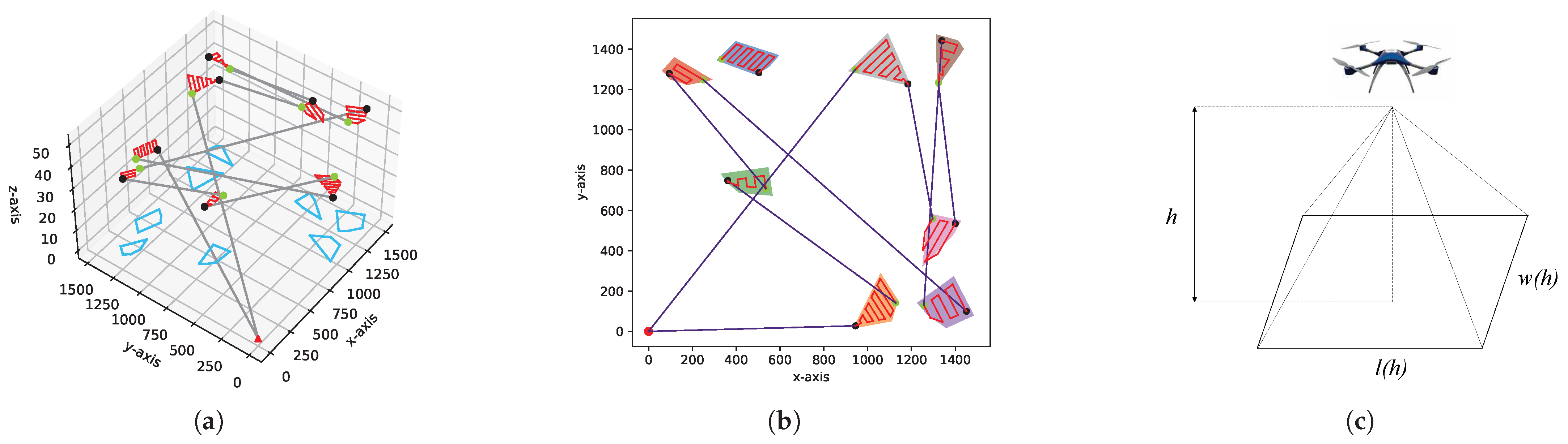
3.1. UAV Visual Coverage Model

In this work, we assume that the UAV carries a camera with a fixed focal length photographic lens, which is usually of superior optical quality, lighter weight, and smaller size, compared with a zoom lens [40]. Image acquisition sensors that are commonly used, such as CMOS sensors, typically have a circular appearance. In this study, we use the central rectangular region of the circular sensor for visual coverage. As shown in Figure 1c, the field of view of the camera is a rectangle. Let f be the focal length, $s_1$ be the horizontal sensor dimension, and $s_2$ be the vertical sensor dimension of the camera. When the UAV’s flight altitude is h, we denote $l\left(h\right)$ and $w\left(h\right)$ as the length and width for the field of view of the camera according to [20] and trigonometry. In particular, we have

$$\begin{array}{c}\hfill l\left(h\right)={\displaystyle \frac{h·s_1}{f}},w\left(h\right)={\displaystyle \frac{h·s_2}{f}}.\end{array}$$

(1)

When using the fixed focal length photographic lens, the UAV may need to adjust its flight altitude to meet the varying image resolution requirements of different regions. Thus, for each region ${\mathcal{P}}_i$, there exists a maximum flight altitude $Z_2^i$ for the UAV to satisfy the minimum image resolution requirement for photographing ${\mathcal{P}}_i$. Also, we assume that there exists a minimum flight altitude $Z_1^i$ for the UAV to meet the safety requirement for photographing ${\mathcal{P}}_i$, e.g., avoiding collisions with tall buildings while flying above the region. On the other hand, we assume that the UAV has its own flight altitude range of $\left[z_1,z_2\right]$, taking into account the UAV’s mechanical properties. Thus, the actual range of the UAV’s flight altitude for photographing each region ${\mathcal{P}}_i$ is denoted as ${\mathcal{R}}_i=\left[z_1,z_2\right]\cap \left[Z_1^i,Z_2^i\right]$. While photographing a certain region ${\mathcal{P}}_i$, we assume that the UAV needs to maintain a fixed flight altitude selected from ${\mathcal{R}}_i$, to guarantee the quality of captured images. In the rest of this paper, we use “photographing altitude” to represent the flight altitude employed by the UAV to photograph a certain region for short.

3.2. UAV Mobility Model

We assume that the UAV can move freely within the 3D space and the real-time location of the UAV is denoted as $L\left(t\right)=\left(x\left(t\right),y\left(t\right),z\left(t\right)\right)$. We denote $V_{\min }^h$ and $V_{\max }^h$ as the minimum and maximum horizontal velocities of the UAV, respectively. We denote $V_{\max }^{\mathrm{a}}$ and $V_{\max }^{\mathrm{d}}$ as the maximum vertical velocities during ascent and descent, respectively. The maximum horizontal and vertical accelerations are denoted as $a_{\max }^h$ and $a_{\max }^v$, respectively. Without loss of generality, we assume that the UAV maintains a constant velocity. In the rest of this paper, we use “velocity” to represent “the UAV’s resultant velocity", if not otherwise specified, while visually covering a certain region (although it may use different constant velocities for different regions), and can continuously change its velocity during the flight between any two neighboring regions. Additionally, the UAV is allowed to decelerate or accelerate at region boundaries if needed, for instance, to adjust its altitude before proceeding to the next region. The total time of a complete visual coverage tour for the UAV can be denoted as

$$\begin{array}{c}\hfill T=T_1+T_2+T_3+T_4,\end{array}$$

(2)

where $T_1$ represents the time from the depot to the entrance point of the first visited region and $T_4$ represents the time from the exit point of the last visited region to the depot. $T_2$ represents the total time the UAV spends on visual coverage over each terrestrial region, during which the UAV maintains a constant altitude and velocity. $T_3$ represents the total flight time of the UAV between adjacent regions, during which it does not perform any visual coverage tasks and is allowed to change its flight altitude and velocity (i.e., the total time taken for the UAV to travel from the exit point of the previous coverage region to the entry point of the next coverage region).

3.3. UAV Flight Energy Consumption Model

According to the law of conservation of energy, we develop the UAV’s flight energy consumption model by comprehensively surveying existing related literature [41,42,43]. Specifically, we divide the UAV’s flight energy consumption into three parts: (1) $E_p$ represents the propulsive energy consumed by the UAV’s power system; (2) $E_h$ represents the energy consumed due to the change in the flight altitude; (3) $E_k$ represents the kinetic energy consumed due to the change of velocity. We assume that the energy consumption of the UAV’s rotors and the camera responsible for visual coverage is negligible in this work, compared with the UAV’s flight energy consumption. In the rest of this paper, we use “energy consumption” to represent “flight energy consumption” for short.

We denote $v\left(t\right)$ as the UAV’s real-time velocity function of time t, then the propulsive power of the UAV is denoted as

$$\begin{array}{c}\hfill P\left(v\left(t\right)\right)=P_0\left(1+{\displaystyle \frac{3v{\left(t\right)}^2}{U_{\mathrm{tip}}^2}}\right)+P_i{\left(\sqrt{1+{\displaystyle \frac{v{\left(t\right)}^4}{4v_0^2}}}-{\displaystyle \frac{v{\left(t\right)}^2}{2v_0^2}}\right)}^{1/2}+{\displaystyle \frac{1}{2}}{d}_0\rho sAv{\left(t\right)}^3,\end{array}$$

(3)

where $P_0$, $U_{\mathrm{tip}}$, $P_i$, $v_0$, $d_0$, $\rho$, s and A are the UAV’s constant mechanical parameters. Specifically, the three components of Equation (3) represent the UAV’s blade profile power, induced power, and parasite power, respectively. Among them, the first and third terms strictly increase monotonically with the UAV’s flight velocity. Thus, during a finite time duration $\left[a,b\right]$, the UAV’s propulsion energy consumption can be calculated as

$$\begin{array}{c}\hfill E_p={\int }_a^{b}P\left(v\left(t\right)\right)dt.\end{array}$$

(4)

It is worth noting that the second term in $P\left(v\left(t\right)\right)$ cannot be precisely integrated using standard integration techniques due to its complex structure. Thus, in this work, we employ the numerical integration method to obtain an approximated integral value with the minimum achievable error.

Due to the change in the UAV’s flight altitude, we denote the corresponding energy consumption as

$$\begin{array}{c}\hfill E_h=M·g·△h,\end{array}$$

(5)

where M represents the mass of the UAV, g is the gravitational acceleration, and $△h$ is the change in the UAV’s flight altitude. Note that $△h$ could be either positive or negative values.

Finally, since the UAV maintains a constant velocity $v_i$ while visually covering any region ${\mathcal{P}}_i$, we only need to consider the change in the UAV’s kinetic energy between any two neighboring regions. Thus, we have

$$\begin{array}{c}\hfill E_k={\displaystyle \frac{M}{2}}\sum _{i=0}^N\left(v_{i+1}^2-v_i^2\right),\end{array}$$

(6)

where $v_0=v_{N+1}=0$.

Based on the above analysis, we calculate the UAV’s total energy consumption during a complete visual coverage tour as follows. Firstly, since the UAV maintains a constant velocity and flight altitude when visually covering a certain region, we only need to consider the propulsion energy for the UAV to visually cover each region ${\mathcal{P}}_i$, which is represented as

$$\begin{array}{c}\hfill E\left(i\right)=P\left(v_i\right)·{\displaystyle \frac{l_i}{v_i}},\end{array}$$

(7)

where $l_i$ represents the length of the intra-region trajectory for visually covering region ${\mathcal{P}}_i$. Secondly, considering the possible changes in flight altitude and velocity, we denote the UAV’s energy consumption used for transition between any two neighboring regions as

$$\begin{array}{c}\hfill E(i,i+1)={\int }_{t_i}^{t_{i+1}}P\left(v\left(t\right)\right)dt+M·g·\left(h_{i+1}-h_i\right)+{\displaystyle \frac{1}{2}}·M·\left(v_{i+1}^2-v_i^2\right),\end{array}$$

(8)

where $t_i$ and $t_{i+1}$ denote the time instants when the UAV leaves the exit point of ${\mathcal{P}}_i$ and arrives at the entrance point of ${\mathcal{P}}_{i+1}$, respectively. We denote $h_i$ and $h_{i+1}$ as the photographing altitudes for visually covering ${\mathcal{P}}_i$ and ${\mathcal{P}}_{i+1}$, respectively. We denote $E(0,1)$ as the UAV’s energy consumption for moving from the depot to the first visited region, and $E(N,N+1)$ represents the UAV’s energy consumption for moving from the last visited region to the depot.

3.4. Problem Formulation

We formulate the joint trajectory design and velocity control problem as follows.

$$\begin{array}{cc}\hfill & min\left[\sum _{i=1}^{N}E\left(i\right)+\sum _{i=0}^{N}E(i,i+1)\right],\hfill \\ \hfill s.t.& T\le T^{*},\hfill \\ \hfill & max\left\{z_1,Z_1^i\right\}\le h_i\le min\left\{z_2,Z_2^i\right\},i\in [1,N],\hfill \\ \hfill & -V_{\max }^d\le {\displaystyle \frac{\mathrm{d}z\left(t\right)}{\mathrm{d}t}}\le V_{\max }^a,t\in [0,T],\hfill \\ \hfill & \left|{\displaystyle \frac{{\mathrm{d}}^{2}z\left(t\right)}{\mathrm{d}{t}^2}}\right|\le a_{\max }^v,t\in [0,T],\hfill \\ \hfill & V_{\min }^h\le ∥\left({\displaystyle \frac{\mathrm{d}x\left(t\right)}{\mathrm{d}t}},{\displaystyle \frac{\mathrm{d}y\left(t\right)}{\mathrm{d}t}}\right)∥\le V_{\max }^h,t\in [0,T],\hfill \\ \hfill & ∥\left({\displaystyle \frac{{\mathrm{d}}^{2}x\left(t\right)}{\mathrm{d}{t}^2}},{\displaystyle \frac{{\mathrm{d}}^{2}y\left(t\right)}{\mathrm{d}{t}^2}}\right)∥\le a_{\max }^h,t\in [0,T],\hfill \end{array}$$

(9)

where $T^{*}$ represents the time it takes for the UAV to finish a visual coverage tour. The second constraint indicates the photographing altitude constraint for visually covering each region. The rest constraints indicate the UAV’s velocity and acceleration constraints in horizontal and vertical directions.

4. The Proposed Method

In this section, we present the proposed four-step approach to designing trajectory and controlling velocity. First, under the constraints of flight safety and image resolution requirements, a modified simulated annealing (SA) algorithm is employed to determine the UAV’s optimal photographing altitude for each terrestrial region. During the search process, suboptimal solutions are accepted with a certain probability, and the algorithm parameters are gradually adjusted to escape local optima and approach a globally optimal set of altitudes. Subsequently, using the altitudes obtained in the previous step and the geometric centroids of the terrestrial regions, the problem is formulated as a Traveling Salesman Problem (TSP). The visitation sequence is then derived using the Christofides algorithm, which guarantees an approximation ratio of 1.5. In the third stage, the Candidate Coverage Path Generation (CCPG) algorithm is utilized to explore all feasible coverage paths within each region, based on their geometric properties and the corresponding UAV altitudes. Finally, leveraging the results from the previous three stages and considering the UAV’s velocity during flight, a dynamic programming (DP) approach is adopted to jointly optimize the UAV’s flight velocity and trajectory, with the objective of minimizing total energy consumption throughout the mission.

4.1. Identifying the Photographing Altitude of Each Region

By comprehensively considering several photographing altitude constraints illustrated in Section 3.1, we define the range of the UAV’s photographing altitude for visually covering each region ${\mathcal{P}}_i$ as

$${\mathcal{R}}_i=\left[H_1^i,H_2^i\right],i=1,2,...N,$$

(10)

where $H_1^i=max\{z_1,Z_1^i\}$ and $H_2^i=min\{z_2,Z_2^i\}$. Based on Equation (10), we need to decide the exact photographing altitude for the UAV to visually cover each region ${\mathcal{P}}_i$, such that the average altitude difference among all regions is minimized. To reduce energy waste caused by frequent climbing or descending between regions, we design the altitude assignment strategy to minimize the average altitude difference among all target regions. This is based on the physical insight that vertical movement, especially climbing, incurs substantial energy consumption due to gravitational potential energy, which increases linearly with altitude change according to Equation (5). In contrast, the potential energy saved by covering each region at its minimum allowable altitude does not always offset the energy cost of drastic altitude transitions. Therefore, by encouraging altitude continuity across regions, we aim to avoid unnecessary vertical maneuvers that dominate energy usage in multi-region UAV coverage missions. Thus, in this work, we developed a simulated annealing (SA)-based searching algorithm [44] to identify the UAV’s photographing altitude of each region, by minimizing the following equation.

$$\begin{array}{c}\hfill H_{\mathrm{diff}}=\sum _{i=1}^N\sum _{j=i+1}^N\left|h_i-h_j\right|.\end{array}$$

(11)

The details can be seen in Algorithm 1. In particular, traditional SA algorithms only output one set of solutions when the algorithm iteration is finished. In this work, we add an external loop process such that the number of solutions output by the proposed algorithm is the same as the number of external loop iterations. From several sets of output solutions, we select the set with the highest average altitude as the final solution in order to enlarge the camera’s shooting range and reduce the intra-region trajectory length accordingly.

Algorithm 1 Identifying the photographing altitude of each region

Require: $N,z_1,z_2,Z_1=\left\{Z_1^i|i\in N\right\},Z_2=\left\{Z_2^i|i\in N\right\}.$ Ensure:  H.  1: $H\leftarrow \varnothing ,\mathbf{R}\leftarrow \varnothing$.  2: //For each region to be covered, corresponding altitude intervals for UAV coverage are defined.  3: for  $i=1\to N$  do  4:    $H_1^i\leftarrow max\left\{z_1,Z_1^i\right\}.$  5:    $H_2^i\leftarrow min\left\{z_2,Z_2^i\right\}.$  6:    $R_i\leftarrow [H_1^i,H_2^i]$.  7:    $\mathbf{R}\leftarrow R_i$  8: end for  9: $ma{x}_{\mathrm{AVR}}\leftarrow 0$.  10: //Based on the obtained altitude intervals, a simulated annealing algorithm is employed to search for a set of coverage altitudes that satisfies the requirements.  11: for  $i=1\to I_1$  do  12:    $output\leftarrow \mathrm{SA}(\mathbf{R},I_2,\alpha ,{\lambda }_1,{\lambda }_0)$.  13:    $AVR\leftarrow \mathrm{aver}\left(output\right)$. // Calculate the average of this set of altitudes.  14:    if $AVR>ma{x}_{\mathrm{AVR}}$ then  15:      $ma{x}_{\mathrm{AVR}}\leftarrow AVR$.  16:      $H\leftarrow output$. // H represents the finally decided set of photographing altitudes.  17:    end if  18: end for

4.2. Deciding the Visiting Order of Each Region

In this section, we optimize the visiting order of each region to generally minimize the traveling distance of the UAV during a complete visual coverage tour. Specifically, we denote the coordinate of the geometric center point of each region ${\mathcal{P}}_i$ as $\left(x_i^g,y_i^g\right)$. Based on the UAV’s photographing altitude $h_i$ decided by Algorithm 1 for each region $P_i$, we construct a set consisting of a number of 3D locations as $\{G_i=\left(x_i^g,y_i^g,h_i\right)|i=1,2,...,N\}$. Then, based on these locations and the depot, we aim to design a path that will pass through each location once with the minimum total path length, which can be formulated as a traveling salesman problem (TSP). The path length between any two neighboring locations is denoted as the Euclidean distance between them, which is shown below.

$$\begin{array}{c}\hfill len\left(G_i,G_j\right)=\sqrt{{\left(x_i^g-x_j^g\right)}^2+{\left(y_i^g-y_j^g\right)}^2+{\left(h_i-h_j\right)}^2}.\end{array}$$

(12)

The TSP has been extensively studied, and can be solved by either approximate or heuristic methods. In this work, we use Christofides’ algorithm [45] with an approximation ratio of $1.5$ to solve the above-formulated TSP. It is worth noting that the generated TSP is only used to decide the UAV’s visiting order of each region, since the resulting visiting order may reduce the overall length of the UAV’s visual coverage tour. The exact flight trajectory of the UAV will be determined in the following two sections.

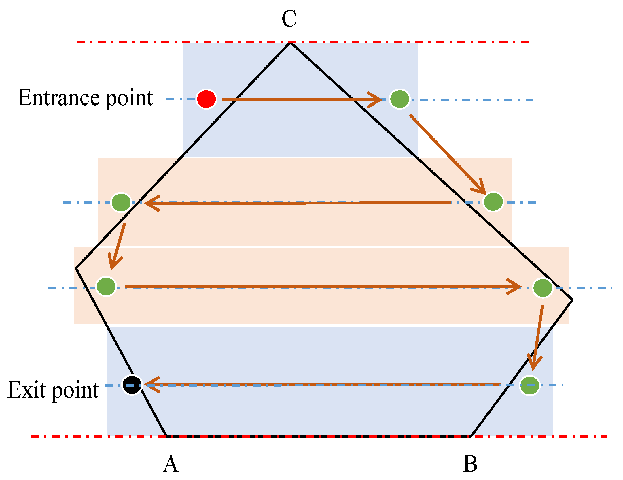
4.3. Generating Candidate Intra-Region Trajectories for Visual Coverage

In this section, we explain how to design the UAV’s trajectory within each region to achieve full visual coverage, which is known as the coverage path planning (CPP) problem [46,47,48,49]. Several methods have been developed to solve the CPP, such as the back-and-forth path (BFP) algorithm [50], candidate coverage path generation (CCPG) algorithm [22], and random path generation algorithm. In this work, we use the CCPG algorithm [22] to generate all candidate intra-region trajectories used for visual coverage of each region, of which the optimal one will be decided together with the inter-region trajectory used to transition between neighboring regions in the next section. Because the inter-region and intra-region trajectories are correlated with each other and cannot be individually optimized.

For example, in Figure 2, we assume that the polygon represents a particular region that needs to be visually covered by the UAV. To find the UAV’s feasible trajectory within the region, the CCPG algorithm operates as follows. First, we randomly select one of the polygon’s edges as the reference edge, i.e., the segment $AB$ in Figure 2. Next, we select one of the polygon’s vertexes that is located the furthest away from $AB$, i.e., point C in Figure 2, as the baseline. Based on segment $AB$ and vertex C, we divide the entire polygon into several subregions, as shown in Figure 2. Thus, the problem of covering an entire region is transformed into a new problem of covering each subregion sequentially. It is worth noting that the entrance point and the exit point of a particular region must be chosen carefully, since both of them affect the specific trajectory for visually covering a region. The pseudocode of CCPG is presented in Algorithm 2.

Algorithm 2 Intra-region path planning for visual coverage

Require: $i,{\mathcal{P}}_i,h_i$. Ensure: $C{P}^i,Q_i$.  1: $Q_i\leftarrow 0$  2: //Each edge of the polygon is traversed to identify all feasible coverage paths within the region.  3: for  $j=1\to d_i$  do  4:    Rotate the edge $\overline{o_{i,j}{o}_{i,j+1}}$ as the reference edge.  5:   Calculate the number of candidate paths $Q_i^j$ based on the selected reference edge and CCPG algorithm [16], and add all candidate paths to the set $C{P}^i$.  6:    $Q_i\leftarrow Q_i+Q_i^j$  7: end for

4.4. Joint Velocity Control and Trajectory Design

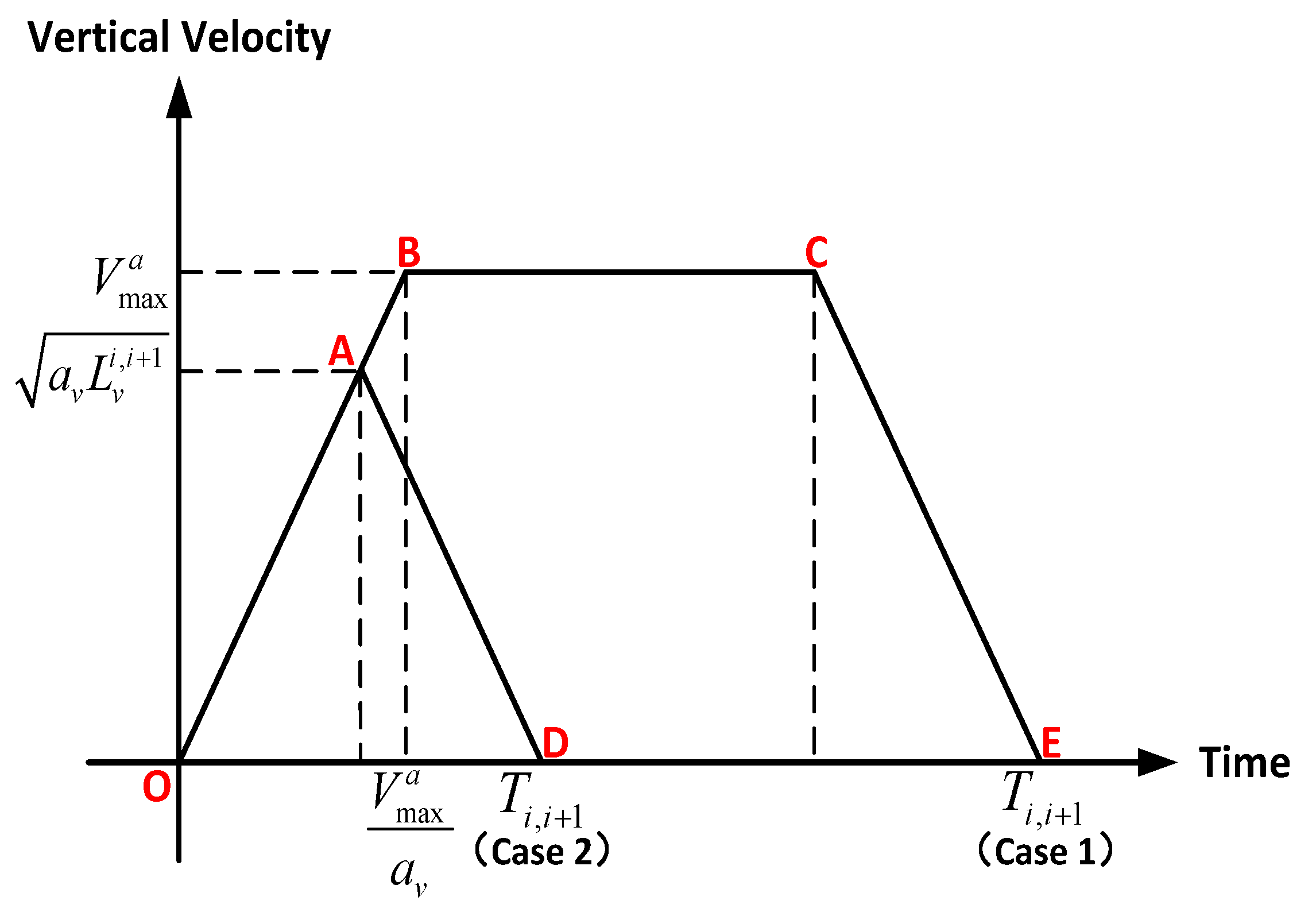
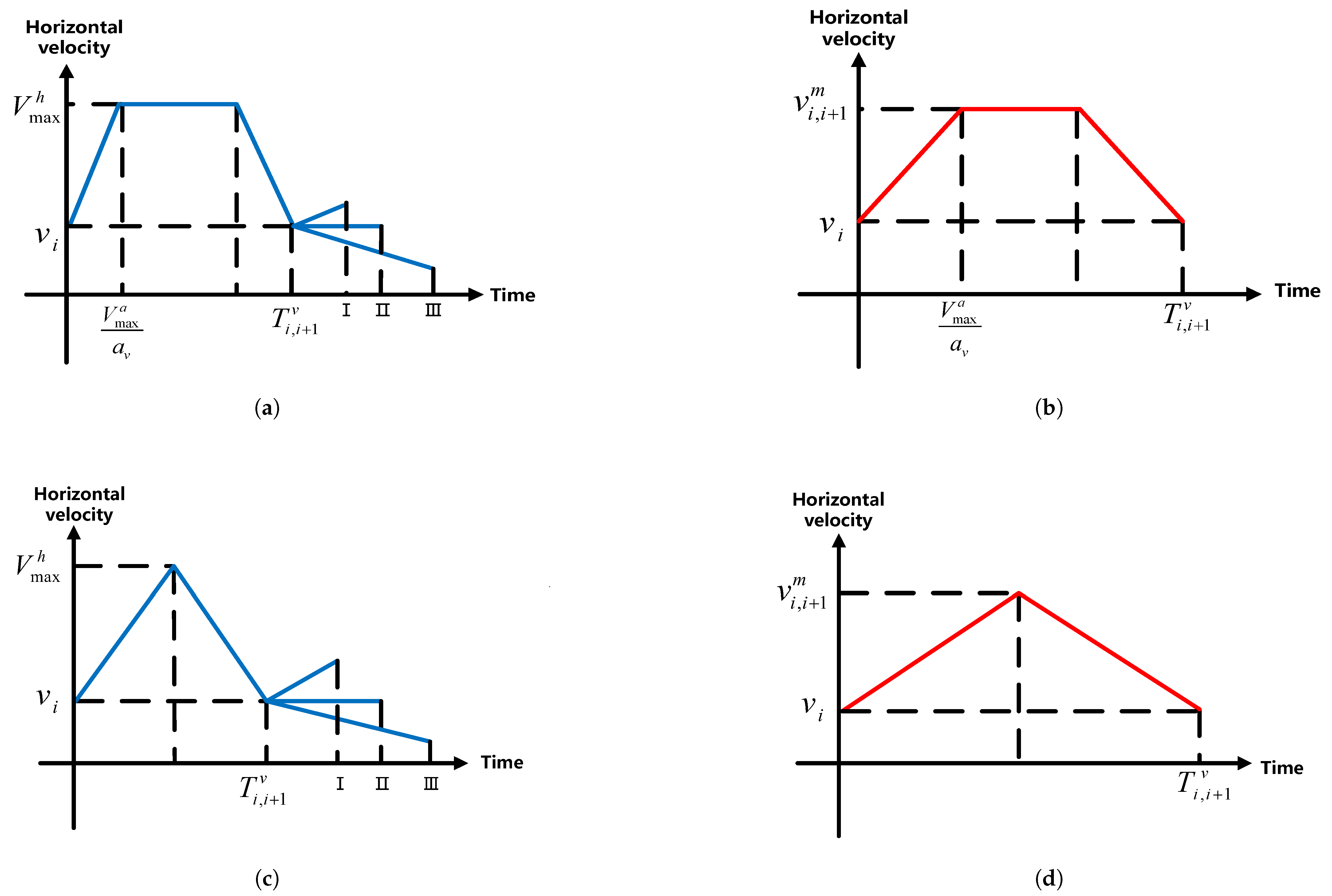
4.4.1. Analysis of UAV Velocity in the Vertical Direction

Considering two neighboring visited regions ${\mathcal{P}}_i$ and ${\mathcal{P}}_{i+1}$, we denote $B_i=\left(x_i^b,y_i^b,h_i\right)$ and $A_{i+1}=\left(x_{i+1}^a,y_{i+1}^a,h_{i+1}\right)$ as the exit point and entrance point of ${\mathcal{P}}_i$ and ${\mathcal{P}}_{i+1}$, respectively. We denote $L_v^{i,i+1}$ as the vertical distance between $B_i$ and $A_{i+1}$. We denote $L_h^{i,i+1}$ as the horizontal distance between $B_i$ and $A_{i+1}$. We analyze the velocity control of the UAV during the transition from $B_i$ to $A_{i+1}$ as follows.

Firstly, in the vertical direction, the UAV remains at zero vertical velocity at both $B_i$ and $A_{i+1}$. Thus, there are two possible cases of vertical velocity change in which the UAV can transition from ${\mathcal{P}}_i$ to ${\mathcal{P}}_{i+1}$, which are shown in Figure 3.

Case 1: When $L_v^{i,i+1}\ge {\displaystyle \frac{{\left(V_{\max }^a\right)}^2}{a_v}}$, i.e., the height difference between $B_i$ and $A_{i+1}$ is relatively large, such that the UAV has sufficient time to accelerate to the maximum vertical velocity before arriving at $A_{i+1}$. In this case, the UAV accelerates to the maximum vertical velocity $V_{\max }^a$, maintains the same velocity for some time, and decelerates to zero vertical velocity. The total time used by the UAV to complete the vertical flight is represented as

$$\begin{array}{c}\hfill T_{i,i+1}^v={\displaystyle \frac{V_{\max }^a}{a_v}}+{\displaystyle \frac{L_v^{i,i+1}}{V_{\max }^a}}.\end{array}$$

(13)

Case 2: When $L_v^{i,i+1}<{\displaystyle \frac{{\left(V_{\max }^a\right)}^2}{a_v}}$, i.e., the height difference between $B_i$ and $A_{i+1}$ is relatively small, such that the UAV does not have sufficient time to accelerate to the maximum vertical velocity before arriving at $A_{i+1}$. In this case, the UAV first accelerates to a certain vertical velocity that is smaller than $V_{\max }^a$, and then decelerates to zero vertical velocity. The total time used by the UAV to complete the vertical flight is represented as

$$\begin{array}{c}\hfill T_{i,i+1}^v=2\sqrt{{\displaystyle \frac{L_v^{i,i+1}}{a_v}}}.\end{array}$$

(14)

Remark: Note that both cases are based on the assumption of $h_{i+1}>h_i$, and the similar results can be derived when $h_{i+1}<h_i$ except that we need to replace $V_{\max }^a$ with $V_{\max }^d$ in both Equations (13) and (14). When $h_{i+1}=h_i$, we have $T_{i,i+1}^v=0$.

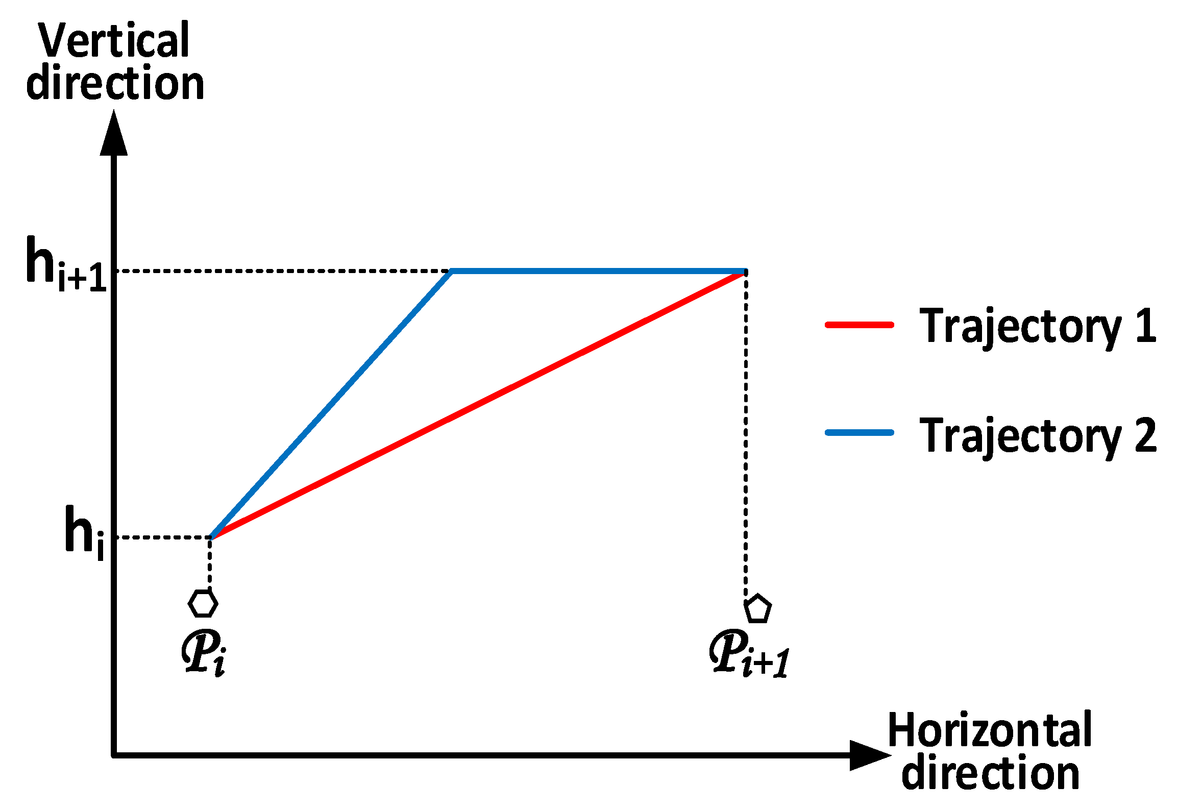
4.4.2. Analysis of UAV Velocity in the Horizontal Direction

Next, based on the above analysis of vertical velocity control, we design the UAV’s horizontal velocity control from $B_i$ to $A_{i+1}$. We denote $T_{i,i+1}^h$ as the total time used by the UAV to transition from $B_i$ to $A_{i+1}$ in the horizontal direction. Since the UAV maintains the same photographing altitude $h_i$ while visually covering region ${\mathcal{P}}_i$, the UAV must complete the altitude change (from $h_i$ to $h_{i+1}$) before arriving at the entrance point $A_{i+1}$ of region ${\mathcal{P}}_{i+1}$. Thus, we conclude that $T_{i,i+1}^h\ge T_{i,i+1}^v$. Otherwise, the UAV has to adjust the photographing altitude during the visual coverage of region ${\mathcal{P}}_{i+1}$, which may affect the stability of the captured image’s quality.

We denote $v_i$ and $v_{i+1}$ as the constant velocities of the UAV while visually covering regions ${\mathcal{P}}_i$ and ${\mathcal{P}}_{i+1}$, respectively.

In Figure 4, we show two possible flight trajectories of the UAV from $B_i$ to $A_{i+1}$, assuming that $h_i\le h_{i+1}$. The red trajectory shows that the UAV completes flights in both horizontal and vertical directions simultaneously. The blue trajectory shows that the UAV first completes the vertical flight, and then maintains the same altitude while flying toward region ${\mathcal{P}}_{i+1}$, which indicates that the horizontal distance between neighboring regions is relatively large, compared with the difference between two photographing altitudes of neighboring regions. Based on Figure 3 and Figure 4, we illustrate four possible changes in the UAV’s horizontal velocity during the transition between neighboring regions in Figure 5.

In particular, we define the critical horizontal distance as $\underline{L_h^{i,i+1}}$, which can be calculated based on the change in the vertical velocity. For the vertical velocity in case 1, we have

$$\begin{array}{c}\hfill \underline{L_h^{i,i+1}}=\left(T_{i,i+1}^v-V_{\max }^a/a_v\right)\left(V_{\max }^h-v_i\right)+v_i·T_{i,i+1}^v.\end{array}$$

(15)

For the vertical velocity in case 2, we have

$$\begin{array}{c}\hfill \underline{L_h^{i,i+1}}={\displaystyle \frac{1}{2}}{T}_{i,i+1}^v\left(V_{\max }^h-v_i\right)+v_i·T_{i,i+1}^v.\end{array}$$

(16)

For example, in Figure 5a, we show the change in the UAV’s horizontal velocity over time during the transition from $B_i$ to $A_{i+1}$, when the corresponding vertical velocity is in case 1 and $L_h^{i,i+1}>\underline{L_h^{i,i+1}}$. Specifically, since the UAV can accelerate to the maximum vertical velocity in case 1, the UAV’s horizontal velocity can also achieve its corresponding maximum value of $V_{max}^h$. After the UAV reaches the altitude of $h_{i+1}$, it can choose to maintain the current velocity, accelerate or decelerate until arriving at $A_{i+1}$, as shown in Figure 5a.

Figure 5b shows the change of the UAV’s horizontal velocity over time during the transition from $B_i$ to $A_{i+1}$, when the corresponding vertical velocity is in case 1 and $L_h^{i,i+1}\le \underline{L_h^{i,i+1}}$, which means that the horizontal distance between $B_i$ and $A_{i+1}$ is not large enough to enable the UAV to accelerate to its maximum horizontal velocity. Thus, in this case, we need to calculate the UAV’s maximum achievable horizontal velocity $v_{i,i+1}^m$ during the transition from $B_i$ to $A_{i+1}$ as follows.

$$\begin{array}{c}\hfill v_{i,i+1}^m={\displaystyle \frac{L_h^{i,i+1}-v_i·T_{i,i+1}^v}{T_{i,i+1}^v-V_{\max }^a/a_v}}+v_i.\end{array}$$

(17)

Similarly in Figure 5c,d, we show the change in the UAV’s horizontal velocity over time during the transition from $B_i$ to $A_{i+1}$, when the corresponding vertical velocity is in case 2. In particular, the UAV’s maximum achievable horizontal velocity in Figure 5d is calculated as follows.

$$\begin{array}{c}\hfill v_{i,i+1}^m={\displaystyle \frac{2(L_h^{i,i+1}-v_i·T_{i,i+1}^v)}{T_{i,i+1}^v}}+v_i.\end{array}$$

(18)

Remark: note that the red and blue curves in Figure 5 indicate that the UAV follows trajectory 1 and trajectory 2 illustrated in Figure 4, respectively.

4.4.3. Joint Optimization of Velocity and Trajectory

Based on the above analysis of the UAV’s velocity change in both vertical and horizontal directions between any two neighboring regions, we employ dynamic programming (DP) to optimize the constant velocity $v_i$ used to visually cover each region ${\mathcal{P}}_i$ as well as the vertical acceleration $a_v^i$ used during the transition between any two neighboring regions ${\mathcal{P}}_i$ and ${\mathcal{P}}_{i+1}$, for minimizing the UAV’s energy consumption.

When the UAV finishes photographing a certain region ${\mathcal{P}}_i$, i.e., it is located at the exit point $B_i$, it first chooses a vertical acceleration from $\left(0,a_{max}^v\right]$. We assume that the discretization factor used to discretize the interval $\left(0,a_{max}^v\right]$ is ${\delta }_1$. Thus, the k-th available vertical acceleration chosen from $\left(0,a_{max}^v\right]$ is denoted as

$$\begin{array}{c}\hfill a_v^{i,k}={\displaystyle \frac{a_{max}^v}{{\delta }_1}}·k.\end{array}$$

(19)

Then, according to Equations (13)–(18) and Figure 4 and Figure 5, we can calculate the time $T_{i,i+1}^v$ required for the UAV to complete the altitude change as well as the maximum achievable horizontal velocity $v_{i,i+1}^m$. Based on Figure 5b,d, we can conclude that if $L_h^{i,i+1}\le \underline{L_h^{i,i+1}}$, the UAV employs the same velocity for visually covering regions ${\mathcal{P}}_i$ and ${\mathcal{P}}_{i+1}$. Otherwise, we denote the j-th available velocity chosen from $\left[V_{\min }^h,V_{\max }^h\right]$ for visually covering ${\mathcal{P}}_{i+1}$ as

$$\begin{array}{c}\hfill v_{i+1}^j=V_{\min }^h+{\displaystyle \frac{V_{\max }^h-V_{\min }^h}{{\delta }_2}}·j,\end{array}$$

(20)

where ${\delta }_2$ is the discretization factor used to discretize the interval $\left[V_{\min }^h,V_{\max }^h\right]$.

We define the UAV’s minimum accumulated energy consumption until when it arrives at $B_{i+1}$, i.e., the exit point of region ${\mathcal{P}}_{i+1}$, as $TE(i+1)$. Then, the state transition equation of DP is constructed as

$$\begin{array}{c}\hfill TE(i+1)=TE\left(i\right)+\min \left[E(i,i+1)+E(i+1)\right].\end{array}$$

(21)

Also, we represent the boundary condition of DP as

$$\begin{array}{c}\hfill TE\left(0\right)=0.\end{array}$$

(22)

Based on Equations (7) and (8), we note that the UAV’s energy consumption is not only related to the velocity control strategy, but is also related to the exact path planning within each region, which includes the exact entrance point, exit point, and the trajectory connecting them. Thus, we need to jointly optimize the velocity control and trajectory design (both intra-region and inter-region). In other words, the UAV’s velocity control and trajectory design are conducted simultaneously, as follows:

$$\begin{array}{c}\hfill v_{i+1},C{P}_{*}^{i+1}=arg\min \left[TE\left(i\right)+\min \left[E(i,i+1)+E(i+1)\right]\right]\end{array}$$

(23)

where $C{P}_{*}^{i+1}$ is the selected intra-region trajectory for visual coverage of region ${\mathcal{P}}_{i+1}$. The detailed DP algorithm for calculating the velocity and trajectory is presented in Algorithm 3 (lines 15–30).

Algorithm 3 Joint velocity control and trajectory design for visual coverage of terrestrial regions

Require: $N,\left\{{\mathcal{P}}_i|i\in N\right\},z_1,z_2,Z_1,Z_2,a_{\max }^v,a_{\max }^h,V_{\max }^d$, $\hspace{1em} V_{\max }^a,V_{\min }^h,V_{\max }^h,{\delta }_1,{\delta }_2$. Ensure: $E,T,tr$.  1: //Select the appropriate photographing altitude of each region.  2: The set of UAV photographing altitudes H is obtained through Algorithm 1.  3: //Determine the visiting order of each region.  4: for  $i=0\to N$  do  5:    for $j=0\to N$ do  6:      Calculate the Euclidean distance $len(G_i,G_j)$ using Equation (12).  7:      $\mathbf{D}\leftarrow len(G_i,G_j)$.  8:    end for  9: end for  10: $\mathbf{OR}=\left\{r\left(i\right)|i\in N\right\}\leftarrow$ Christofides$(\left\{{\mathcal{P}}_i|i\in N\right\},\mathbf{D})$. //$r\left(0\right)=0$ means the UAV starts from the depot.  11: //Determine the velocity control and trajectory design for the UAV to perform a complete visual coverage tour.  12: for  $i=1\to N$  do  13:    Calculate $C{P}^i,Q_i$ using Algorithm 2.  14: end for  15: $E\leftarrow 0,T\leftarrow 0,tr\leftarrow \varnothing ,\mathbf{V}\leftarrow \varnothing$.  16: for  $i=0\to N$  do  17:    //We consider the situation when the UAV returns from the last visited region to the depot separately.  18:    if $i\le N$ then  19:      for $k=1\to {\delta }_1$ do  20:         Based on the selected $a_v^{i,k}$ and Figure 3, Figure 4 and Figure 5, analyze the UAV’s velocity and trajectory between neighboring regions.  21:         for $j=1\to Q_{r(i+1)}$ do  22:           //Consider all feasible intra-region trajectories for ${\mathcal{P}}_{r(i+1)}$.  23:           Based on Equations (7), (8) and (23), calculate the UAV’s minimum accumulated energy consumption $TE\left(i+1\right)$ until when finishes visually covering ${\mathcal{P}}_{r(i+1)}$; calculate the time $T_{i,i+1}$ used for the UAV to move from the exit point of ${\mathcal{P}}_{r\left(i\right)}$ to the exit point of ${\mathcal{P}}_{r(i+1)}$.  24:         end for  25:      end for  26:      $E\leftarrow TE(i+1),T\leftarrow T+T_{i,i+1},tr\leftarrow tr\bigcup C{P}_{*}^{i+1}\bigcup C{P}_{i,i+1},\mathbf{V}\leftarrow v_{i+1}$. //$C{P}_{i,i+1}$ represents the inter-region trajectory of the UAV between ${\mathcal{P}}_{r\left(i\right)}$ and ${\mathcal{P}}_{r(i+1)}$.  27:    else  28:      After the UAV finishes visually covering the last region, we assume that the next region to be visually covered is the depot, and the corresponding velocity is 0.  29:    end if  30: end for

4.5. Computational Complexity Analysis of Algorithm 3

We show the complete pseudo code of the UAV’s velocity control and trajectory design in Algorithm 3 by incorporating Algorithms 1 and 2. Line 2 shows the process of selecting the photographing altitude of each region. Lines 4–10 show the process of deciding the visiting order of each region. Lines 12–14 show the process of obtaining all feasible intra-region trajectories for visually covering each region. Lines 15–30 show DP iterations of joint velocity control and trajectory design of the UAV. Some variables used in Algorithms 1–3 are presented in

Table 2. Main notations used in Algorithms 1–3.

Notation	Definition
${\delta }_1,{\delta }_2$	The discretization factors of DP
$tr$	The UAV’s complete flight trajectory
H	The set of photographing altitudes of all regions
$\mathbf{D}$	The set of Euclidean distance between each pair of geometric center points of neighboring regions
$\mathbf{OR}$	The visiting order of each region
${\mathcal{P}}_{r\left(i\right)}$	The i-th region visited by the UAV
$\mathbf{V}$	The set of velocities used to cover each region
$\alpha$	The cooling rate of SA
$d_i$	The total number of edges of region ${\mathcal{P}}_i$
$\overline{o_{i,j}{o}_{i,j+1}}$	The edge formed by connecting the j-th vertex and the (j + 1)-th vertex of region ${\mathcal{P}}_i$
$C{P}_j^i$	The j-th candidate path within region ${\mathcal{P}}_i$
$Q_i$	The total number of candidate paths within region ${\mathcal{P}}_i$
${\lambda }_1,{\lambda }_0$	The final and initial temperature of SA
$I_2,I_1$	The number of internal and external loops of SA

.

Next, we discuss the computational complexity of Algorithm 3. For the process of deciding the photographing altitude of each region by the developed SA-based searching algorithm (i.e., Algorithm 1), the corresponding complexity is calculated as $O\left(I_1·I_2·⌈{log}_{\alpha }{\displaystyle \frac{{\lambda }_1}{{\lambda }_0}}⌉\right)$, where $I_1$ is the number of external loop iterations, $I_2$ is the number of internal loop iterations, $\alpha$ is the cooling rate, ${\lambda }_0$ is the initial temperature, and ${\lambda }_1$ is the stopping temperature. For the process of deciding the visiting order of each region by the Christofides algorithm [45], the corresponding complexity is calculated as $O\left(N^3\right)$.

The computational complexity of Algorithm 2 depends on the geometric features of each region. For any region ${\mathcal{P}}_i$, we denote the largest distance between any two points within the region as ${ϵ}_i$ and let $ϵ=\underset{1\le i\le N}{max}{ϵ}_i$. In addition, we denote $h^{\prime }$ as the lowest photographing altitude of the UAV among all regions, where $h^{\prime }=\underset{1\le i\le N}{min}{h}_i$. Thus, the complexity of Algorithm 2 is calculated as $O\left(ϵ·h^{\prime }·{\sum }_{i=1}^N{Q}_i^2\right)$.

The computational complexity of DP iterations is decided by the number of subproblems and the computational complexity of each subproblem. In this work, the number of subproblems of DP equals to the number of regions, which is N. The computational complexity of each subproblem depends on the discretization factors adopted by the proposed DP. Let $Q_m=\underset{1\le i\le N}{max}{Q}_i$, then the computational complexity of DP iterations is $O\left({\delta }_1·{\delta }_2·Q_m·N\right)$.

In summary, the computational complexity of Algorithm 3 is $O\left(I_1·I_2·⌈{log}_{\alpha }{\displaystyle \frac{{\lambda }_1}{{\lambda }_0}}⌉\right)+O\left(N^3\right)+O\left(ϵ·h^{\prime }·{\sum }_{i=1}^N{Q}_i^2\right)+O\left({\delta }_1·{\delta }_2·Q_m·N\right)=O\left(N^3\right)$ with respect to the number of terrestrial regions N.

4.6. Limitations and Approximate Optimality

Given the complexity of the proposed problem—which includes jointly optimizing the UAV’s photographing altitude, region visiting sequence, intra-region coverage path, and velocity profile—the overall problem is inherently NP-hard, incorporating discrete decisions (e.g., visiting order) and continuous optimization (e.g., altitude selection and velocity selection). To address this in a tractable manner, we decompose the problem into four sequential stages, each optimized using tailored algorithms.

This heuristic decomposition does not guarantee global optimality, as decisions made in earlier stages (e.g., altitude assignment via simulated annealing) are not revisited after downstream constraints (e.g., routing or velocity) are introduced. For instance, the altitude selection is guided by minimizing inter-region altitude variation—a proxy that simplifies vertical energy consideration—but this may not always align perfectly with minimizing total energy, especially if more aggressive altitude shifts could reduce horizontal flight distance.

Nevertheless, our design isolates the major energy-affecting factors: altitude selection primarily impacts vertical energy cost and image quality, while the routing and DP-based trajectory optimization govern horizontal movement and dynamic acceleration. By tackling these subproblems independently, we achieve a practical balance between solution quality and computational efficiency.

While the current approach sacrifices theoretical guarantees of optimality, it enables scalable planning across larger problem instances and provides a flexible framework that can be further refined through adaptive feedback or joint optimization strategies in future work.

5. Evaluation

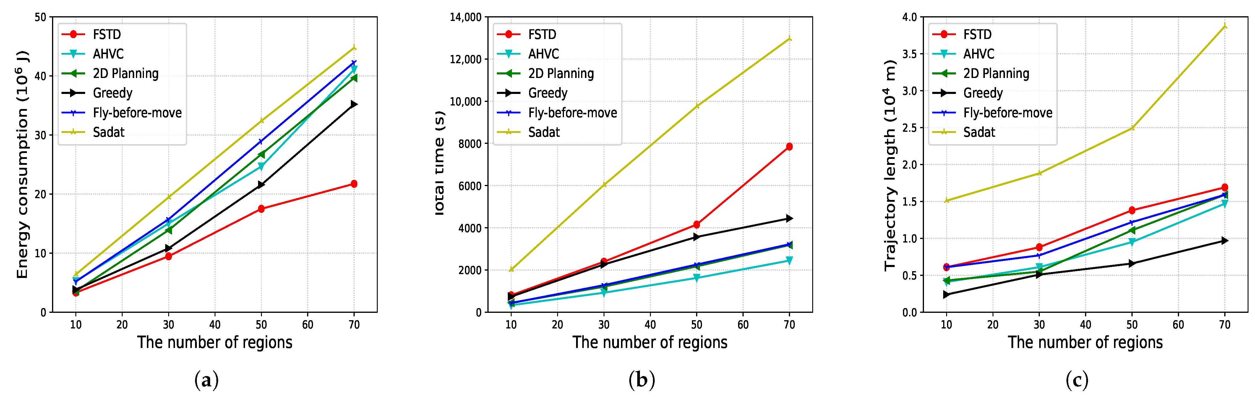
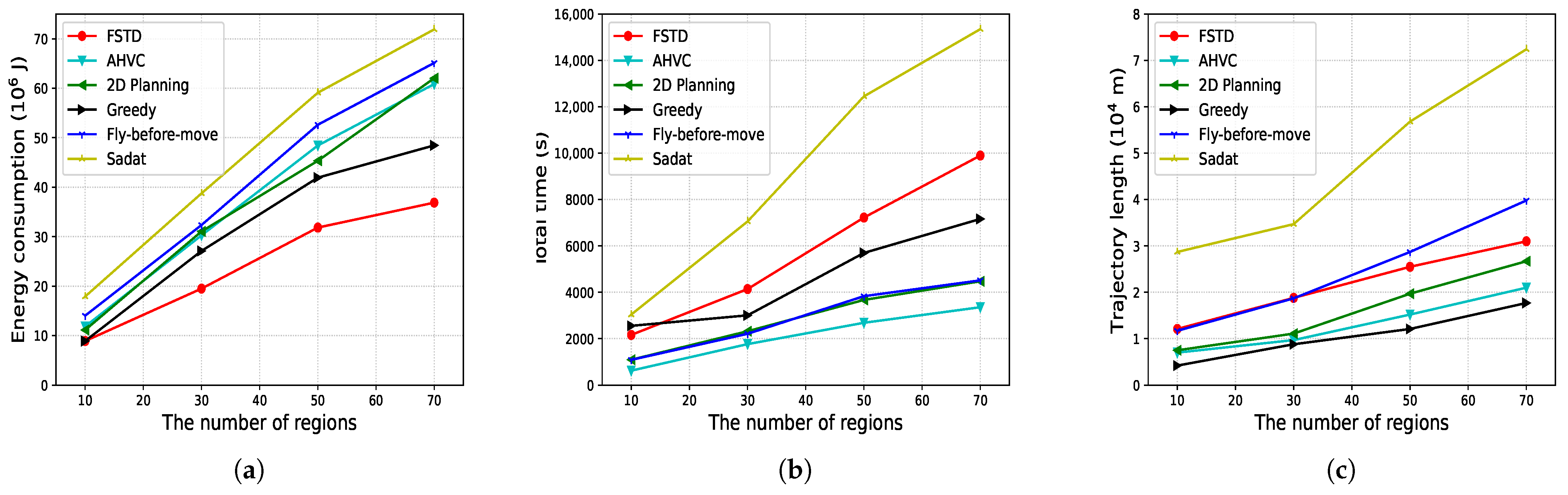
5.1. Experiment Setting

The values of the UAV’s mechanical parameters used for simulation are shown in

Table 3. Values of the UAV’s mechanical parameters used for simulation.

Notation	Definition	Value
M	The mass of the UAV	10
g	The gravity acceleration	9.8
A	Rotor disc area	0.79
s	Rotor solidity	0.05
$d_0$	Fuselage drag ratio	0.3
$v_0$	Mean rotor induced velocity in hover	7.2
$U_{tip}$	Tip speed of the rotor blade	200
$P_0$	Coefficient in the propulsion power formula	580
$P_i$	Coefficient in the propulsion power formula	1438

(all values are expressed in standard units). In addition, the maximum vertical and horizontal accelerations of the UAV are set to $a_{max}^v=3\mathrm{m}/{\mathrm{s}}^2$ and $a_{max}^h=8\mathrm{m}/{\mathrm{s}}^2$, respectively. The UAV’s maximum ascending and descending velocities are set to $V_{max}^a=5\mathrm{m}/\mathrm{s}$ and $V_{max}^d=3\mathrm{m}/\mathrm{s}$, respectively. The UAV’s minimum and maximum horizontal velocities are set to $V_{min}^h=3\mathrm{m}/\mathrm{s}$ and $V_{max}^h=15\mathrm{m}/\mathrm{s}$, respectively. In this experiment, we use two different photographic lenses for the UAV’s camera, where one of them has a focal length of $f=36$ mm, horizontal sensor dimension of $s_1=38$ mm, and vertical sensor dimension of $s_2=25$ mm; the other one has a focal length of $f=27$ mm, horizontal sensor dimension of $s_1=13$ mm, and vertical sensor dimension of $s_2=7.5$ mm. The number of edges of any terrestrial polygon is sampled from $\left[3,8\right]$.

In particular, we conduct the experiment in two different scenarios: (1) Scenario 1 is conducted in a square area of 800 m × 800 m and there are N regions randomly distributed in this area, where $N=$10, 30, 50, and 70. In this scenario, the UAV carries the camera with parameters of $f=36$ mm, $s_1=38$ mm, and $s_2=25$ mm; (2) Scenario 2 is conducted in a square area of 1500 m × 1500 m with the same setting of number of regions as in Scenario 1. In this scenario, the UAV carries the camera with parameters of $f=27$ mm, $s_1=13$ mm, and $s_2=7.5$ mm. The resolution requirement of each region in both scenarios is randomly generated. For the parameter setting of Algorithm 1, the initial temperature is set to 1000, the final temperature is set to 10, and the cooling rate is set to $0.99$. Also, the internal loop of the algorithm runs for 50 iterations and the external loop runs for 10 iterations.

For the sake of clarity in the subsequent discussion, the proposed algorithm is hereinafter referred to as FSTD (four-step trajectory design). To validate the effectiveness and superiority of the proposed algorithm in this work, we use the following algorithms as benchmarks for performance comparison.

Table 4. Features of benchmark algorithms.

Algorithm	Key Features	Objective
AHVC	Max velocity and max altitude per region	Minimize total mission time
2D Planning	Fixed altitude (minimum allowed), constant velocity	Simplified planning ignoring altitude and speed variability
Greedy	Chooses next region with minimum incremental energy	Myopic local energy optimization
Fly-before-move	Performs vertical then horizontal flight sequentially	Decouples movement phases, simplified control
Sadat	DFS/BFS-based region subdivision with frequent altitude reset	Fractal-style coverage, high altitude variation

offers a succinct overview of the key features of these benchmark algorithms.

• Attaining heterogeneous visual coverage (AHVC): Based on [22], this method requires the UAV to fly at the maximum allowable velocity and the highest permissible altitude for each region. Its primary objective is to minimize the total mission time, rather than energy consumption.
• Two-dimensional planning: This baseline assumes a constant flight altitude (set to the minimum allowable altitude) and fixed velocity throughout the entire mission. The UAV plans a 2D TSP-style tour, ignoring altitude or speed variations, which simplifies trajectory planning but sacrifices adaptability [29].
• Greedy: A heuristic algorithm where, after completing the coverage of a region, the UAV selects the next unvisited region that results in the minimum incremental energy cost. This myopic strategy is simple but may lead to suboptimal global solutions.
• Fly-before-move: In this strategy, the UAV decouples vertical and horizontal movement. It first ascends or descends to the required altitude, then proceeds with horizontal flight to the next region. This sequential treatment of vertical and planar motion may cause inefficient transitions and higher energy usage.
• Sadat: Inspired by the fractal coverage approach in [51], this method uses breadth-first or depth-first search (BFS/DFS) to cover each region, which is divided into multiple sub-regions. After covering each subregion, the UAV must return to the maximum altitude before proceeding to the next one, leading to frequent altitude changes and potentially increased energy consumption.

5.2. Performance Comparison

In Figure 6, we compare the proposed algorithm with other five algorithms with respect to the UAV’s energy consumption, task completion time, and trajectory length, respectively, in Scenario 1. The UAV flight energy consumption of the six algorithms under two scenarios is presented in

Table 5. Energy consumption for 50 regions.

	FSTD	AHVC	2D Planning	Greedy	Fly-Berore-Move	Sadat
Scenario 1	17.50	24.67	26.73	21.57	29.00	32.37
Scenario 2	31.84	48.43	45.34	41.93	52.62	59.10

and

Table 6. Energy consumption for 70 regions.

	FSTD	AHVC	2D Planning	Greedy	Fly-Berore-Move	Sadat
Scenario 1	21.73	41.06	39.65	35.19	42.29	44.75
Scenario 2	36.87	60.85	62.03	48.45	65.12	71.90

. We present the UAV’s energy consumption when the number of terrestrial regions is 50 and 70. The data in the tables are in units of ${10}^6$ J and are rounded to two decimal places.

In Figure 6a, the results show that our algorithm outperforms the other five benchmark algorithms in terms of the energy consumption when the number of regions varies from 10 to 70. In particular, when there are 70 regions, our algorithm reduces the energy consumption by $45.8\%$ on average, compared with the other five benchmark algorithms.

In Figure 6b, we can see that the AHVC algorithm achieves the minimum task completion time of the UAV, compared with other comparative algorithms, since the AHVC algorithm requires the UAV to employ the maximum allowable velocity during the entire visual coverage tour. Our algorithm performs relatively well, especially when there are less than 50 regions. After all, it is highly challenging to make trades between the UAV’s task completion time and energy consumption, since they are inherently contradictory.

In Figure 6c, we can see that the Greedy algorithm, 2D Planning algorithm, and AHVC algorithm achieve relatively short trajectories, while our algorithm and the “fly-before-move” algorithm achieve longer trajectories. In particular, the Sadat algorithm achieves a much longer trajectory, compared with the other five comparative algorithms, due to the frequent changes in the UAV’s flight altitude during its visual coverage of each region.

We have also conducted the performance comparison in Scenario 2 and the corresponding results are shown in Figure 7, which are generally consistent with those in Scenario 1. In terms of algorithm runtime, we compared the performance of six algorithms under Scenario 1. As shown in Figure 8, under the same hardware conditions (CPU: Intel i7-8750H, Memory: 16GB, DELL laptop (Dell Inc., Jinhua, Zhejiang, China)), all algorithms except the Sadat algorithm completed their calculations within 30 s. Our proposed method, which incorporates heuristic progress, has a longer runtime compared to the other four algorithms.

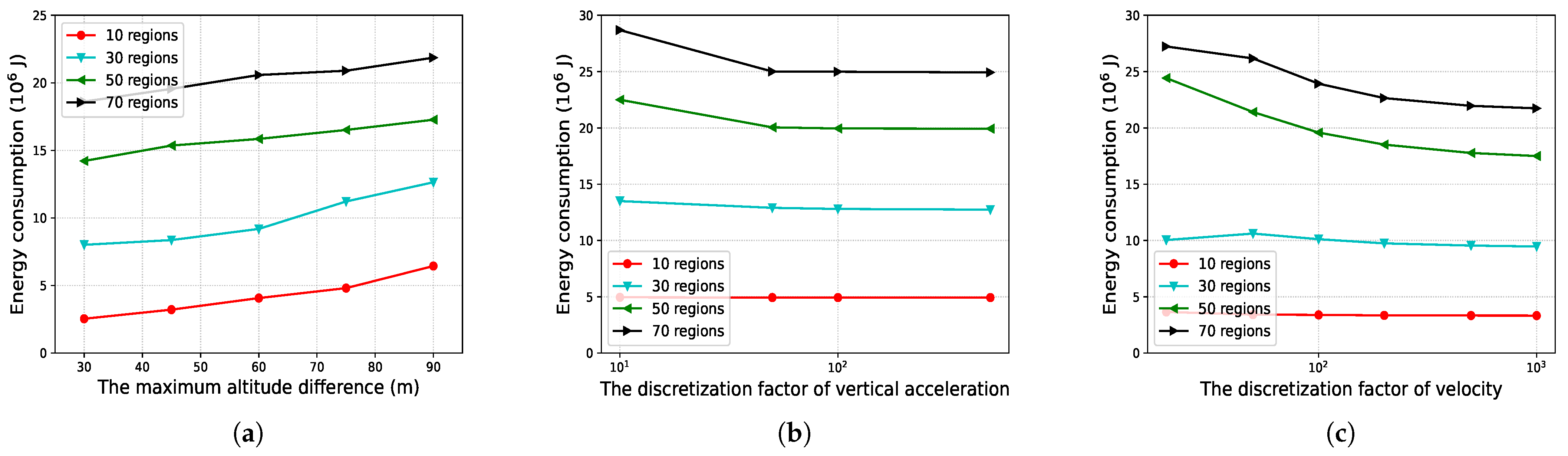
5.3. Impacts of System Parameters on Our Algorithm

In this section, we study the impacts of several system parameters on the UAV’s energy consumption achieved by the proposed algorithm in Scenario 1.

In Figure 9a, we explore the impact of the maximum altitude difference among all regions on the UAV’s energy consumption. The results show that the UAV’s energy consumption increases with the maximum altitude difference among all regions in all cases when the number of regions is set to 10, 30, 50, and 70, respectively.

In Figure 9b, we investigate the impact of the discretization factor of the vertical acceleration used in DP iterations on the UAV’s energy consumption. The results show that the UAV’s energy consumption is less affected by the discretization factor of the vertical acceleration when the number of regions is small. However, when the number of regions is larger, we can see that the UAV’s energy consumption decreases significantly with the discretization factor of the vertical acceleration. In addition, in all cases when the number of regions is set to 10, 30, 50, and 70, respectively, the UAV’s energy consumption first decreases and then converges when the discretization factor of the vertical acceleration exceeds 100.

In Figure 9c, we investigate the impact of the discretization factor of the velocity in DP iterations on the UAV’s energy consumption. Results show that the UAV’s energy consumption decreases significantly with the discretization factor of the velocity when the number of regions is set to 50 and 70, respectively. Similar to the results in Figure 8b, the UAV’s energy consumption is less affected by the discretization factor of the velocity when the number of regions is set to 10 and 30. In general, in all cases when the number of regions is set to 10, 30, 50, and 70, respectively, the UAV’s energy consumption first decreases and then converges when the discretization factor of the velocity exceeds 500.

The experimental results presented in Figure 9 collectively highlight the significant role of fine-grained control over both velocity and altitude in improving the UAV’s energy efficiency. In particular, as the discretization levels of vertical acceleration and velocity increase, the UAV gains greater flexibility to adapt its motion more precisely, leading to reduced energy consumption. This is especially evident in scenarios with a larger number of regions, where trajectory complexity increases and coarse discretization may lead to suboptimal or abrupt maneuvers.

Such flexibility becomes even more crucial in complex and dynamic environments, where terrain variability and the presence of obstacles necessitate continuous adaptation. The ability to adjust altitude within a wider range allows the UAV to maintain optimal viewing conditions while avoiding energy-costly maneuvers. Similarly, a broader and more refined velocity space enables smoother transitions and energy-aware acceleration or deceleration, which significantly reduces unnecessary power expenditure during flight.

Therefore, integrating flexible altitude and velocity adjustment not only enhances energy efficiency but also improves the UAV’s adaptability and robustness in real-world deployment scenarios. This underscores the necessity of incorporating such flexibility in future UAV mission planning algorithms, especially when dealing with dynamically changing operational constraints.

6. Conclusions

In this work, we studied the issue of using a UAV to visually cover several terrestrial regions with the minimum energy consumption. To address this issue, we proposed a novel approach that is composed of four steps. The first step selected the UAV’s photographing altitude for each visited region, taking into account various requirements of image resolution and safety across regions. The second step used a TSP-based approximate solution to determine the visiting order of each region, according to the identified photographing altitudes. The third step provided candidate visual coverage trajectories for all regions, based on which the final step employed DP and geometry to jointly determine the UAV’s velocity and trajectory during its complete task tour. The results of the experiments demonstrated that the proposed approach outperforms existing methods in terms of the UAV’s energy consumption.

Looking ahead, several promising directions for future research can be identified. First, integrating real-time environmental data—such as weather conditions, terrain variations, or the presence of obstacles—could enable adaptive trajectory adjustments, further enhancing energy efficiency in dynamic environments. Second, the proposed approach could be optimized for specific mission requirements, such as search and rescue or agricultural monitoring, where mission constraints differ from standard visual coverage tasks. Thirdly, an interesting extension is to consider multi-UAV collaboration, where multiple drones coordinate to cover regions in parallel with lower per-UAV energy usage; this introduces new challenges in communication, load balancing, and joint path planning. Finally, online or adaptive planning strategies could be explored, where the UAV updates its route in real time in response to unexpected changes in the environment or task demands (e.g., newly added or canceled regions).

These extensions would not only increase the robustness of the framework but would also broaden its applicability in real-world scenarios requiring responsiveness and scalability. Investigating the applicability of this methodology in other UAV applications, such as mapping, logistics, or disaster assessment, could also provide valuable insights into its broader use and effectiveness across various domains.

References

1. Mozaffari, M.; Saad, W.; Bennis, M.; Nam, Y.-H.; Debbah, M. A tutorial on UAVs for wireless networks: Applications, challenges, and open problems. IEEE Commun. Surv. Tutor. 2019, 21, 2334–2360. [Google Scholar] [CrossRef]
2. Niu, G.; Cao, Q.; Chen, C.S. Vision-based target localization with cooperative UAVs towards indoor surveillance. In Proceedings of the 2023 IEEE 98th Vehicular Technology Conference (VTC2023-Fall), Hong Kong, 10–13 October 2023; pp. 1–6. [Google Scholar]
3. Liu, X.; Chen, M.; Zhangchen, X.; Tang, Y.; Fang, Y.; Shi, X.; Xu, Z. Intelligent UAV platform: Assist construction of agricultural production automation. In Proceedings of the 2022 7th International Conference on Intelligent Computing and Signal Processing (ICSP), Xi’an, China, 15–17 April 2022; pp. 1009–1012. [Google Scholar]
4. Sotheara, S.; Aso, K.; Aomi, N.; Shimamoto, S. Effective data gathering and energy-efficient communication protocol in wireless sensor networks employing UAV. In Proceedings of the 2014 IEEE Wireless Communications and Networking Conference (WCNC), Istanbul, Turkey, 6–9 April 2014; pp. 2342–2347. [Google Scholar]
5. Kucherov, D.; Shmelova, T.; Poshyvailo, O.; Tkachenko, V.; Miroshnichenko, I.; Ogirko, I. Mathematical model of damping of UAV oscillations in the cargo delivery problem. In Proceedings of the 2023 IEEE 4th KhPI Week on Advanced Technology (KhPIWeek), Kharkiv, Ukraine, 2–6 October 2023; pp. 1–6. [Google Scholar]
6. Petrlík, M.; Báča, T.; Heřt, D.; Vrba, M.; Krajník, T.; Saska, M. A robust UAV system for operations in a constrained environment. IEEE Robot. Autom. Lett. 2020, 5, 2169–2176. [Google Scholar] [CrossRef]
7. Saha, S.; Aich, S.; Saha, N.; Saha, S.; Chakraborty, R.; Bishnu, S.K. Deploying UAVs equipped with LIDAR for the quantification of tree biomass and the systematic classification of arboreal species. In Proceedings of the 2025 8th International Conference on Electronics, Materials Engineering and Nano-Technology (IEMENTech), Kolkata, India, 31 January–2 February 2025; pp. 1–7. [Google Scholar]
8. Dong, F.; Li, L.; Lu, Z.; Pan, Q.; Zheng, W. Energy-efficiency for fixed-wing UAV-enabled data collection and forwarding. In Proceedings of the 2019 IEEE International Conference on Communications Workshops (ICC Workshops), Shanghai, China, 20–24 May 2019; pp. 1–6. [Google Scholar]
9. Paredes, J.A.; Saito, C.; Abarca, M.; Cuellar, F. Study of effects of high-altitude environments on multicopter and fixed-wing UAVs’ energy consumption and flight time. In Proceedings of the 2017 13th IEEE Conference on Automation Science and Engineering (CASE), Xi’an China, 20–23 August 2017; pp. 1645–1650. [Google Scholar]
10. Zhan, C.; Lai, H. Energy minimization in Internet-of-Things system based on rotary-wing UAV. IEEE Wirel. Commun. Lett. 2019, 8, 1341–1344. [Google Scholar] [CrossRef]
11. Yan, H.; Chen, Y.; Yang, S.-H. New energy consumption model for rotary-wing UAV propulsion. IEEE Wirel. Commun. Lett. 2021, 10, 2009–2012. [Google Scholar] [CrossRef]
12. Zhan, C.; Huang, R. Energy efficient adaptive video streaming with rotary-wing UAV. IEEE Trans. Veh. Technol. 2020, 69, 8040–8044. [Google Scholar] [CrossRef]
13. Wang, Y.; Wang, Y.; Ren, B. Energy saving quadrotor control for field inspections. IEEE Trans. Syst. Man, Cybern. Syst. 2022, 52, 1768–1777. [Google Scholar] [CrossRef]
14. Ribeiro, P.; Coelho, A.; Campos, R. On the energy consumption of rotary-wing and fixed-wing UAVs in flying networks. In Proceedings of the 2025 20th Wireless On-Demand Network Systems and Services Conference (WONS), Tyrol, Austria, 27–29 January 2025; pp. 1–4. [Google Scholar]
15. Bianchi, D.; Borri, A.; Di Gennaro, S.; Preziuso, M. UAV trajectory control with rule-based minimum-energy reference generation. In Proceedings of the 2022 European Control Conference (ECC), London, UK, 12–15 July 2022; pp. 1497–1502. [Google Scholar]
16. Mathur, A.; Atkins, E. Multi-mode flight simulation and energy-aware coverage path planning for a lift+cruise QuadPlane. Drones 2025, 9, 287. [Google Scholar] [CrossRef]
17. Xiong, Y.; Lu, M.; Chen, W. Modeling and maximizing angle coverage in visual sensor networks. In Proceedings of the 2018 37th Chinese Control Conference (CCC), Wuhan, China, 25–27 July 2018; pp. 2406–2409. [Google Scholar]
18. Zheng, C.; Yin, H.; Li, J.; Lu, M. A multi-objective evolutionary algorithm for shortest path with maximal visual coverage. In Proceedings of the 2011 International Conference on Intelligent Computation and Bio-Medical Instrumentation, Wuhan, China, 14–17 December 2011; pp. 232–235. [Google Scholar]
19. Yen, H.-H. Efficient visual sensor coverage algorithm in Wireless Visual Sensor Networks. In Proceedings of the 2013 9th International Wireless Communications and Mobile Computing Conference (IWCMC), Sardinia, Italy, 1–5 July 2013; pp. 1516–1521. [Google Scholar]
20. Kumar, N.; Ghosh, M.; Singhal, C. UAV network for surveillance of inaccessible regions with zero blind spots. In Proceedings of the IEEE INFOCOM 2020—IEEE Conference on Computer Communications Workshops (INFOCOM WKSHPS), Toronto, ON, Canada, 6–9 July 2020; pp. 1213–1218. [Google Scholar]
21. Xu, C.; Liao, X.; Tan, J.; Ye, H.; Lu, H. Recent research progress of unmanned aerial vehicle regulation policies and technologies in urban low altitude. IEEE Access 2020, 8, 74175–74194. [Google Scholar] [CrossRef]
22. Ko, Y.-C.; Gau, R.-H. UAV velocity function design and trajectory planning for heterogeneous visual coverage of terrestrial regions. IEEE Trans. Mob. Comput. 2023, 22, 6205–6222. [Google Scholar] [CrossRef]
23. Tnunay, H.; Moussa, K.; Hably, A.; Marchand, N. Virtual leader based trajectory generation of UAV formation for visual area coverage. In Proceedings of the IECON 2021—47th Annual Conference of the IEEE Industrial Electronics Society, Toronto, ON, Canada, 13–16 October 2021; pp. 1–6. [Google Scholar]
24. Wang, H.; Zhang, S.; Zhang, X.; Zhang, X.; Liu, J. Near-optimal 3-D visual coverage for quadrotor unmanned aerial vehicles under photogrammetric constraints. IEEE Trans. Ind. Electron. 2022, 69, 1694–1704. [Google Scholar] [CrossRef]
25. Zhu, X.; Zhou, M. Maximal weighted coverage deployment of UAV-enabled rechargeable visual sensor networks. IEEE Trans. Intell. Transp. Syst. 2023, 24, 11293–11307. [Google Scholar] [CrossRef]
26. Liao, J.; Zhang, J.; Zhang, H.; Zhou, L.; Xu, C. DRED: A DRL-based energy-efficient data collection scheme for UAV-assisted WSNs. In Proceedings of the 2022 IEEE 22nd International Conference on Communication Technology (ICCT), Nanjing, China, 11–14 November 2022; pp. 846–851. [Google Scholar]
27. Wu, S.; Dai, H.; Liu, L.; Xu, L.; Xiao, F.; Xu, J. Cooperative scheduling for directional wireless charging with spatial occupation. IEEE Trans. Mob. Comput. 2024, 23, 286–301. [Google Scholar] [CrossRef]
28. Lin, C.; Guo, C.; Dai, H.; Wang, L.; Wu, G. Near optimal charging scheduling for 3-D wireless rechargeable sensor networks with energy constraints. In Proceedings of the 2019 IEEE 39th International Conference on Distributed Computing Systems (ICDCS), Dallas, TX, USA, 7–9 July 2019; pp. 624–633. [Google Scholar]
29. Xie, J.; Garcia Carrillo, L.R.; Jin, L. Path planning for UAV to cover multiple separated convex polygonal regions. IEEE Access 2020, 8, 51770–51785. [Google Scholar] [CrossRef]
30. Wang, H.; Song, S.; Guo, Q.; Xu, D.; Zhang, X.; Wang, P. Cooperative motion planning for persistent 3D visual coverage with multiple quadrotor UAVs. IEEE Trans. Autom. Sci. Eng. 2024, 21, 3374–3383. [Google Scholar] [CrossRef]
31. Huang, Z.; Wang, S. Joint visual coverage and energy consumption optimization for UAV-aided 5G-and-beyond communications. IEEE Trans. Veh. Technol. 2024, 73, 19417–19431. [Google Scholar] [CrossRef]
32. Zhao, P.; Zhang, Y.; Zhang, K.; Bian, K.; Song, L. Optimal trajectory planning for UAV-relayed dynamic spectrum access. In Proceedings of the 2018 IEEE International Symposium on Dynamic Spectrum Access Networks (DySPAN), Seoul, Republic of Korea, 22–25 October 2018; pp. 1–5. [Google Scholar]
33. Wen, W.; Luo, K.; Liu, L.; Zhang, Y.; Jia, Y. Joint trajectory and pick-up design for UAV-assisted item delivery under no-fly zone constraints. IEEE Trans. Veh. Technol. 2023, 72, 2587–2592. [Google Scholar] [CrossRef]
34. Lumbantoruan, H.; Adachi, K. Trajectory and communication protocol for efficient data collecting in UAV-enabled WSN. In Proceedings of the 2020 International Conference on Information Networking (ICOIN), Barcelona, Spain, 7–10 January 2020; pp. 348–353. [Google Scholar]
35. Gong, J.; Chang, T.-H.; Shen, C.; Chen, X. Flight time minimization of UAV for data collection over wireless sensor networks. IEEE J. Sel. Areas Commun. 2018, 36, 1942–1954. [Google Scholar] [CrossRef]
36. Dandapat, J.; Gupta, N.; Agarwal, S.; Kumbhani, B. Service time maximization for data collection in multi-UAV-aided networks. IEEE Trans. Intell. Veh. 2024, 9, 328–337. [Google Scholar] [CrossRef]
37. Dai, X.; Duo, B.; Yuan, X.; Renzo, M.D. Energy-efficient UAV communications in the presence of wind: 3D modeling and trajectory design. IEEE Trans. Wirel. Commun. 2024, 23, 1840–1854. [Google Scholar] [CrossRef]
38. Silvirianti; Shin, S.Y. Energy-efficient multidimensional trajectory of UAV-aided IoT networks with reinforcement learning. IEEE Internet Things J. 2022, 9, 19214–19226. [Google Scholar] [CrossRef]
39. Tan, L.; Zhang, G. Trajectory planning and energy optimization for UAV-assisted vehicular networks in urban scenarios. In Proceedings of the 2022 IEEE 8th International Conference on Computer and Communications (ICCC), Chengdu, China, 9–12 December 2022; pp. 758–764. [Google Scholar]
40. PhotographyLife. Prime vs Zoom Lenses. PhotographyLife 2025. Available online: https://photographylife.com/prime-vs-zoom-lenses (accessed on 11 November 2023).
41. Li, B.; Na, Z.; Liu, R.; Lin, B. Energy consumption minimization of rotary-wing UAVs for data distribution. IEEE Commun. Lett. 2023, 27, 1819–1823. [Google Scholar] [CrossRef]
42. Zeng, Y.; Wu, Q.; Zhang, R. Accessing from the sky: A tutorial on UAV communications for 5G and beyond. Proc. IEEE 2019, 107, 2327–2375. [Google Scholar] [CrossRef]
43. Zeng, Y.; Xu, J.; Zhang, R. Energy minimization for wireless communication with rotary-wing UAV. IEEE Trans. Wirel. Commun. 2019, 18, 2329–2345. [Google Scholar] [CrossRef]
44. Wu, L.; Sun, Q.; Xu, H.; Song, X.; Zhang, Y. Design of hybrid simulated annealing algorithm for UAV scheduling based on coordinated task scheduling. In Proceedings of the 2021 40th Chinese Control Conference (CCC), Shanghai, China, 26–28 July 2021; pp. 1669–1674. [Google Scholar]
45. Zhang, Q.; Xu, W.; Liang, W.; Peng, J.; Liu, T.; Wang, T. An improved algorithm for dispatching the minimum number of electric charging vehicles for wireless sensor networks. Wirel. Netw. 2019, 25, 1371–1384. [Google Scholar] [CrossRef]
46. Galceran, E.; Carreras, M. A survey on coverage path planning for robotics. Robot. Auton. Syst. 2013, 61, 1258–1276. [Google Scholar] [CrossRef]
47. Gajjar, S.; Bhadani, J.; Dutta, P.; Rastogi, N. Complete coverage path planning algorithm for known 2D environment. In Proceedings of the 2017 2nd IEEE International Conference on Recent Trends in Electronics, Information & Communication Technology (RTEICT), Bangalore, India, 19–20 May 2017; pp. 963–967. [Google Scholar]
48. Zhou, Y.; Sun, R.; Yu, S.; Sun, Y.; Sun, L. A complete coverage path planning algorithm for cleaning robots based on the distance transform algorithm and the rolling window approach in dynamic environments. In Proceedings of the 2017 IEEE 7th Annual International Conference on CYBER Technology in Automation, Control, and Intelligent Systems (CYBER), Honolulu, HI, USA, 31 July–4 August 2017; pp. 1335–1340. [Google Scholar]
49. Zheng, Y.; Tu, X.; Yang, Q. Optimal multi-agent map coverage path planning algorithm. In Proceedings of the 2020 Chinese Automation Congress (CAC), Shanghai, China, 6–8 November 2020; pp. 6055–6060. [Google Scholar]
50. Vasquez-Gomez, J.I.; Marciano-Melchor, M.; Valentin, L.; Herrera-Lozada, J.C. Coverage path planning for 2D convex regions. J. Intell. Robot. Syst. 2020, 97, 81–94. [Google Scholar] [CrossRef]
51. Sadat, S.A.; Wawerla, J.; Vaughan, R. Fractal trajectories for online non-uniform aerial coverage. In Proceedings of the 2015 IEEE International Conference on Robotics and Automation (ICRA), Seattle, WA, USA, 26–30 May 2015. [Google Scholar]
Figure 1. SystemModel. (a) 3D trajectory of the UAV. (b) Projection of the UAV’s 3D trajectory on the ground. (c) The UAV’s visual coverage model.
Drones 09 00339 g001
Figure 2. An example of intra-region trajectory design for visual coverage of a region.
Drones 09 00339 g002
Figure 3. The UAV’s vertical velocity change during the transition between neighboring regions.
Drones 09 00339 g003
Figure 4. Two possible flight trajectories for the UAV to transition between neighboring regions.
Drones 09 00339 g004
Figure 5. The UAV’s horizontal velocity change between neighboring regions. (a) When the vertical velocity is case 1 and L h i , i + 1 > L h i , i + 1 ̲ . (b) When the vertical velocity is case 1 and L h i , i + 1 L h i , i + 1 ̲ . (c) When the vertical velocity is case 2 and L h i , i + 1 > L h i , i + 1 ̲ . (d) When the vertical velocity is case 2 and L h i , i + 1 L h i , i + 1 ̲ .
Drones 09 00339 g005
Figure 6. Performance comparison in Scenario 1 regarding the energy consumption, task completion time, and trajectory length. (a) Energy consumption. (b) Total time of visual coverage tour. (c) Trajectory length.
Drones 09 00339 g006
Figure 7. Performance comparison in Scenario 2 regarding the energy consumption, task completion time, and trajectory length. (a) Energy consumption. (b) Total time of visual coverage tour. (c) Trajectory length.
Drones 09 00339 g007
Figure 8. Execution time of the algorithms in Scenario 1.
Drones 09 00339 g008
Figure 9. Impacts of system parameters on the performance of our algorithm in Scenario 1. (a) The impact of the maximum altitude difference on energy consumption. (b) The impact of the discretization factor of vertical acceleration on energy consumption. (c) The impact of discretization factor of velocity on energy consumption.
Drones 09 00339 g009