Abstract
In recent decades, forests have experienced an increasing trend in the number of pest outbreaks worldwide, apparently driven by strong annual variability in precipitation, higher air temperatures, and strong winds. Pest outbreaks have negative ecological, economic, and environmental impacts on forest ecosystems, such as reduced biodiversity, carbon sequestration, and overall forest health. Traditional monitoring methods of these disturbances, while accurate, are time-consuming and limited in scope. Remote sensing, particularly UAV (Unmanned Aerial Vehicle)-based technologies, offers a precise and cost effective alternative for monitoring forest health. This study evaluates the temporal and spatial progression of bark beetle damage in a fir-dominated forest in the Zao Mountains, Japan, using UAV RGB imagery and DL (Deep Learning) models (YOLO - You Only Look Ones), over a four-year period (2021–2024). Trees were classified into six health categories: Healthy, Light Damage, Medium Damage, Heavy Damage, Dead, and Fallen. The results revealed a significant decline in healthy trees, from 67.4% in 2021 to 25.6% in 2024, with a corresponding increase in damaged and dead trees. Light damage emerged as a potential early indicator of forest health decline. The DL model achieved an accuracy of 74.9% to 82.8%. The results showed the effectiveness of DL in detecting severe damage but highlighted that challenges in distinguishing between healthy and lightly damaged trees still remain. The study highlights the potential of UAV-based remote sensing and DL for monitoring forest health, providing valuable insights for targeted management interventions. However, further refinement of the classification methods is needed to improve accuracy, particularly in the precise detection of tree health categories. This approach offers a scalable solution for monitoring forest health in similar ecosystems in other subalpine areas of Japan and the world.
1. Introduction
Forests worldwide are increasingly affected by the growing frequency and intensity of forest insect pest and disease outbreaks, driven in part by climate change [1,2,3]. These disturbances have profound ecological, economic, and environmental consequences, threatening forest biodiversity, carbon sequestration, and the overall ecosystem [4,5,6,7]. Bark beetles, in particular, have become a significant agent of disturbance, with outbreaks causing widespread damage to forests around the globe [8,9]. Their activity is exacerbated by prolonged droughts and rising temperatures, which weaken tree defenses and create ideal conditions for severe infestations [4,6,10].
Traditional methods for monitoring and detecting bark beetle outbreaks, such as ground-based field surveys, German slot traps, and the use of multispectral satellite imagery come with significant limitations, namely spatial resolution, acquisition frequency, and cost. These approaches are also time-intensive, geographically constrained, and often require specialized equipment. Consequently, they may fail to capture the full extent of infestations over large areas [11,12,13,14].
Remote sensing techniques, particularly UAV (Unmanned Aerial Vehicle)-based methods, have emerged as a viable alternative in recent years. UAVs offer broad spatial coverage, high-quality resolution, and low monitoring costs [11,15,16]. They have become an essential tool to investigate forest areas [17,18,19]. UAV-based remote sensing has proven particularly useful for tracking forest disturbances, such as those caused by bark beetles, as it allows for a detailed site-specific analysis of tree health and mortality at the individual tree level [11].
While UAVs provide an abundance of high-quality data, manual interpretation remains a challenge, as expert-based assessments are subjective, require high levels of knowledge, and are costly [12,20]. To address this, deep learning (DL) algorithms have been increasingly applied to automate the detection and classification of tree health [21,22,23]. DL models, particularly convolutional neural networks (CNNs), have demonstrated exceptional performance in extracting patterns from UAV-acquired imagery and have outperformed traditional machine learning approaches used in forest health monitoring [16,24,25].
Previous research has used UAV [21,26,27,28,29,30,31,32,33] and satellite [34,35] imagery for forest monitoring, often with simpler classification schemes and a variety of reported results. In contrast, based on DL models, our study applies a more detailed and complex approach to better capture forest health variability.
UAVs together with DL models have proven particularly effective in monitoring bark beetle infestations [36,37]. UAV-based imagery allows detailed mapping of healthy, infested, and dead trees, even at early infestation stages. Satellite imagery covers large areas, but compared to UAV-based images are low in resolution and can limit the detection of details, especially in forests [38]. This capability is important for understanding the spatial and temporal dynamics of pest outbreaks, enabling timely management interventions. DL algorithms further enhance the efficiency of data analysis, automating the classification of tree health conditions and improving the accuracy of damage detection. Recent studies have demonstrated the potential of UAV-based methods combined with DL for detecting forest disease and pest infestations using UAV-based RGB images [37,39]. However, challenges such as varying weather conditions and the need for high-quality data remain critical issues for effective ecosystem monitoring.
The aim of this study is to assess the spatial and temporal distribution of healthy, damaged, and dead fir trees in the Zao Mountains, Japan, during the period 2021 to 2024, using computer vision and DL. This forest was severely affected by bark beetle outbreaks. Over the past decade, the infestation has spread, causing significant damage and continued degradation of the forest ecosystem [10,11,40].
2. Materials and Methods
2.1. Study Site
The study area is located in the Zao Mountains, a volcanic region in the southeast of Yamagata Prefecture, Japan, 38°09′05″ N, 140°25′03″ E. The mountains are part of the Ou mountain range that extends across the northeast region of Honshu, the main island of Japan (Figure 1). The selected study site covers approximately 25 hectares and lies at an elevation between 1332 m and 1733 m. The terrain is characterized by steep slopes and dense natural vegetation, consisting of a mix of coniferous and deciduous trees. In the lower parts, the vegetation is a mixed forest; this changes with elevation to a mono-culture (Figure 2).
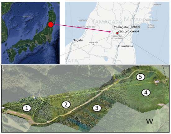
Figure 1.
Study area in Zao Mountains, northeast of Japan, with the separated sub-study sites. The numbers represent the names of several sub-areas of our study.
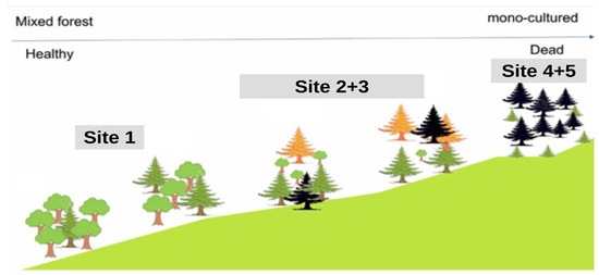
Figure 2.
Cross-section of our study site in Zao Mountains. The figure shows a simple distribution of the infested trees from site 1 to site 5, as well as the species, distribution, and density of the vegetation.
The area is predominantly covered by Maries fir (Abies mariesii), which occurs in both pure and mixed stands, accounting for about 87% of the vegetation. Other common tree species in the region include Fagus crenata, Acer japonicum, Ilex crenata, Chengiopanax sciadophylloides, Taxus cuspidata, Pinus spp., Acer tschonoskii, Cornus controversa, Quercus crispula, and Sorbus commixta. The average tree density is approximately 300 fir trees per hectare, with species composition, density, and individual tree size varying with increasing elevation (Figure 2). The fir trees in the areas are mainly between 41 and 103 years old, with an average age of 72 years. The diameter at breast height ranges from 18 to 40 cm [41]. The study area is divided into five sites (hereafter referred to as sites 1, 2, 3, 4, and 5) along an elevation gradient ranging from 1332 m to 1670 m. Site 1 (3.9 ha) is located at the lowest elevation, site 5 (6 ha) is situated at the highest point. At lower elevations (sites 1 and 2), in addition to Maries fir, various deciduous tree species such as Acer spp., Fagus crenata, and Sorbaria sorbifolia are present. However, with increasing elevation, the proportion of deciduous trees decreases, leaving almost exclusively Maries fir trees dominating the middle elevations (site 3). At sites 4 and 5 (1508–1670 m), environmental stress and insect infestations have led to the death of 95% of the Maries fir population.
Site 1, located at a relatively low elevation, is characterized by a mix of Maries fir and deciduous species. This site exhibits better tree health compared to higher elevations. Since 2012, a massive outbreak of the Tortrix moth (Epitonia piceae Issiki (Lepidoptera: Tortricidae)) has caused significant defoliation, which weakened fir trees that were further attacked by bark beetles (Polygraphus proximus Blandford (Coleoptera: Curculionidae, Scolytinae)), leading to widespread tree mortality. For verifying the correct species, the bark beetle adults were morphologically identified using specific dichotomous keys and by comparison with voucher specimens deposited in our laboratory. The morphological observations confirmed that the investigated species was P. proximus. Another important characteristic of the study area is the competition between Maries firs and subalpine shrub species for resources. While active regeneration of the fir trees would suppress the spread of shrubs, the limited natural regeneration has allowed shrubs to increasingly dominate the region (Figure 2).
2.2. Climate
The winter months are particularly cold, with average temperatures ranging between −10 °C and −5 °C from December to February. Zao is also well known for its significant snowfall, with snow depths averaging between 150 and 200 cm during these months. In some years, peak values of up to 260 cm have been recorded, especially in February and March. In spring, temperatures begin to rise, and the snow cover gradually decreases; while significant snow cover is still present in March and April, the snow completely melts by May. On the west slope, snow melt is almost one month earlier than on the east slope. During spring, temperatures range between 0 °C and 10 °C. The summer months, from July to August, are relatively mild, with average temperatures between 16 °C and 19 °C. Autumn (September to November) brings cooler temperatures, ranging from 5 °C to 15 °C. Snowfall usually begins again in November, although the snow depth in late autumn remains moderate, ranging between 5 and 50 cm. Zao receives approximately 1450 mm of annual precipitation. The climate data presented here are sourced from the Zao weather station and the website weather-and-climate.com. The climate in Zao exhibits strong seasonal variability, characterized by cold, snowy winters and mild summers.
2.3. Drones
The primary data used in this study are UAV-acquired RGB images. Due to the evolution of this technology and the availability during the study period, we employed three different UAV models (Figure 3) for data collection: DJI Phantom 4 RTK, DJI Mavic 2 Pro, and DJI Mavic 3 Multispectral. The following technical specifications are relevant for the captured image data. The DJI Phantom 4 RTK is equipped with a 1-inch CMOS sensor (20 MP). The camera features a focal length of 8.8 mm (equivalent to 24 mm) and a maximum resolution of 5472 × 3648 pixels. It uses a mechanical shutter to avoid distortions caused by the rolling shutter effect. Images are captured with a field of view (FOV) of 84°. Additionally, the drone is equipped with an RTK (real-time kinematic) module, enabling high-precision georeferencing. The DJI Mavic 2 Pro has a Hasselblad L1D-20c camera with a 1-inch CMOS sensor (20 MP). The focal length is 10.26 mm (equivalent to 28 mm), with a field of view (FOV) of 77°. The camera offers a variable aperture ranging from f/2.8 to f/11 and can capture images with a maximum resolution of 5472 × 3648 pixels. The DJI Mavic 3 Multispectral features an RGB camera with a 4/3 CMOS sensor (20 MP). The focal length is 24 mm (equivalent) with a field of view (FOV) of 84°. The maximum image resolution is 5280 × 3956 pixels. Additionally, the drone includes a multispectral camera with five sensors (green, red, red-edge, near-infrared, and RGB), each with a resolution of 5 MP.

Figure 3.
The UAVs used in this study. From left to right: DJI Phantom 4 RTK, DJI Mavic 2 Pro, DJI Mavic 3 MS.
2.4. Data Collection and Processing
To achieve comparable results over time, the same flight plans were consistently used for each data collection flight. The UAV flights were conducted at an altitude of 90 m using the “following terrain” function to maintain a consistent ground sampling distance. An image overlap of 85% frontal and lateral was chosen to ensure high-quality orthomosaics. Additionally, flights were scheduled on days with stable weather conditions, avoiding periods of strong sunlight or adverse weather, such as fog, heavy rain, or strong winds. Data collection was carried out at regular intervals, ensuring comparability across similar dates each year. For this study, images were captured across various seasons, primarily in June, August, and October, between 2021 and 2024. The data were collected using different UAV platforms: Mavic 2 Pro used without RTK, resulting in lower georeferencing accuracy; Phantom 4 and Mavic 3 Multispectral using RTK, which provided high-precision georeferencing. No ground control points (GCPs) were used for any of the flights.
For the processing and analysis of the image data, several specialized software solutions were used. The software Metashape (Agisoft LLC, Saint Petersburg, Russia) was used for processing the RGB images from the UAV flights into orthomosaics. This program facilitated the creation of high-resolution orthomosaics and the georeferenced post-processing data. We generated 20 orthomosaics, stored in JPG or TIFF format, with a pixel size ranging from 0.014 m to 0.021 m. The coordinate system Tokyo_UTM_Zone_54N was used.
After data processing (Figure 4c), manual annotations of the different tree health categories (Figure 4i) was performed, while the steps for DL application went from “d” to “h” (Figure 4c,d). ArcGIS Pro (ESRi, Inc., LLC, Redlands, CA, USA) was utilized for the analysis of the generated geodata. Trees were manually annotated (point features), and classified into the different classes. The manual annotation helped track changes over time, providing insights into forest dynamics, tree health, and spatial distribution. The manual annotations were based on the level of defoliation.
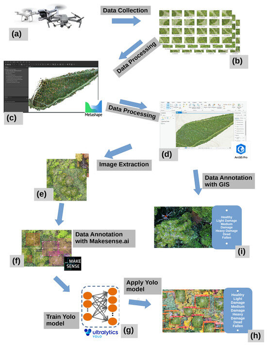
Figure 4.
Study workflow. (a,b) Collecting and storing of data; (c) processing with Metashape [Agisoft LLC]; (d,e,i) post-processing in ArcGIS Pro [ESRI Inc], as well as annotating; (f) annotation of DL data with Makesence.ai [S.Growth, vers. 1.11.0]; (g,h) training, use, and analysis with the YOLO8n model.
The dataset contains 6 tree health categories (Figure 5a–f). In order to improve the performance of the classification steps of the YOLO network, two dummy categories were added: Artificial Object and Human (Figure 5g,h). The tree health categories were as follows: Healthy (no defoliation), Light Damage (up to 20% defoliation), Medium Damage (21–50%), Heavy Damage (over 50%), Dead (100%), and Fallen (tree laying on ground).
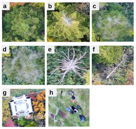
Figure 5.
Examples of the 6 main categories and 2 dummy classes. Main classes: (a)—Healthy, (b)—Light Damage, (c)—Medium Damage, (d)—Heavy Damage, (e)—Dead, and (f)—Fallen. Dummy classes: (g)—Artificial Object, (h)—Human. The six main categories were also used in the manual annotation.
From the 20 generated orthomosaics, patches, which were used as datasets for training, validation, and testing of the DL model, were randomly extracted with GIS software. The annotation of the dataset for the DL model was performed using MakeSense.ai, a web-based platform from Skalski Growth (Krakow, Poland), which was used for the manual labeling of image content. The form of the annotations were boxes around each represented tree in the image. In total, 5176 patches, varying in resolution, environmental conditions, shape, and pixel size were used, while 1789 patches were classified as background images and contained no annotations. The dataset contains 25597 annotations including all categories (Table 1). The images were randomly divided into 80% for the training dataset and 20% for the validation dataset, not considering any class balancing.

Table 1.
Summary of all annotations of the 8 categories. The numbers of annotations in the training dataset and in the validation dataset.
The test dataset comprises four plots (each measuring 50 m × 50 m) located within an orthomosaic generated in September 2024 (Figure 6). Neither the plots nor the orthomosaic were used in the training or validation of the DL model, ensuring an independent evaluation. The true data (verified tree annotations) of the dataset from this orthomosaic consisted of 330 trees with annotations of the 6 main categories (Table 2).
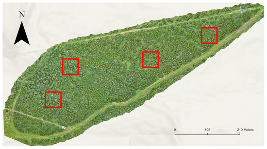
Figure 6.
Selected plots (4 red squares) in Site 2 (September 2024, Orthomosaic).
Table 2.
True data of YOLO test dataset.
Data augmentation plays a crucial role in enhancing the original dataset by generating additional training samples. This technique is essential for balancing under-represented categories. In this study, augmentation was applied especially on images containing the Heavy Damage category. Each such image was augmented up to two times to compensate for class imbalance. To achieve this, vertical and horizontal flipping were applied, which is equivalent to mirroring the images along the respective axis. By flipping the images, the dataset was artificially expanded, helping to address the category imbalance (Table 1). It is important to highlight that augmentation was not restricted solely to areas where heavy-damage trees were found, but was systematically applied whenever an under-represented class was present in the image. As long as at least one tree in a patch belonged to this category, the image underwent augmentation. With that, all other categories in the images were automatically augmented since the whole image was flipped. Notably, data augmentation was deliberately excluded from the test dataset to ensure an unbiased evaluation. As a result, a total of 393 images were augmented through flipping (mirroring), effectively doubling their count.
Another category is “Vanishing Logs”, which are not visible anymore after several years. These were once fallen trees, but over time they decayed or became overgrown with vegetation, eventually rendering them undetectable (Figure 7). These data were not used in the DL.
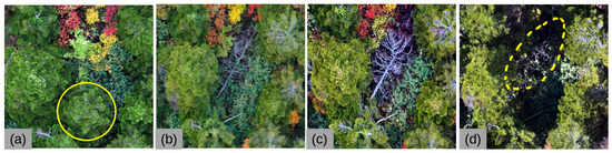
Figure 7.
Temporal evolution of a tree from healthy (yellow cycle) to fallen to not visible (yellow dashed circle) from October 2021 to 2024: healthy (a); fallen (b) and (c); not visible (d).
2.5. Deep Learning
In this study, we used YOLO version 8 (YOLOv8n), a state-of-the-art object detection model from the Ultralytics YOLOv8 series. YOLO is an algorithm that revolutionized the field by framing detection as a single regression problem [42,43]. Unlike traditional methods that use complex pipelines involving region proposals and multiple stages, YOLO processes the entire image in one forward pass through a convolutional neural network (CNN). It divides the input image into a grid, and each grid cell is responsible for predicting bounding boxes, confidence scores, and class probabilities for objects whose centers fall within that cell. By combining these predictions, YOLO efficiently localizes and classifies objects in real time, achieving an impressive balance between speed and accuracy. This unified approach makes YOLO particularly suitable for applications requiring fast and reliable object detection [43].
A key advantage of using YOLOv8n is its ability to perform both tree detection and classification in a single step, eliminating the need for separate annotation efforts outside this study. This significantly reduced the time-consuming task of manual labeling.
The model was trained for 500 epochs using customized settings tailored for automated object detection. An image size of 800 and a batch size of 1 were used. The optimizer was set to SGD (Stochastic Gradient Descent) with a learning rate of 0.01 and a momentum of 0.9. Training was conducted on the captured image dataset to ensure robust performance in identifying and classifying trees. The training data were used in their original form, without any prior normalization or resampling. Upon completing the training process, the YOLO model was deployed to evaluate the test dataset.
2.6. Deep Learning Analysis
The categorization performance of the DL model was evaluated using a confusion matrix, which included six distinct categories: Healthy, Light Damage, Medium Damage, Heavy Damage, Dead, and Fallen. In the calculation of the performance metrics, these categories were treated as separate categories, allowing for a detailed assessment of the model’s capability to distinguish between varying stages of tree health and degradation. To complement this fine-grained evaluation and enhance interpretability, the model’s performance was also assessed using aggregated categories. Specifically, Light Damage, Medium Damage, and Heavy Damage were combined into a single category referred to as Damage, while the Dead and Fallen classes were merged into a category termed Decay. The Healthy category remained unchanged and was retained across both classification schemes. This dual-level categorization, differentiating between separate and aggregated classes, allowed for a more comprehensive and robust evaluation of the model. It provided insights not only into the model’s performance in categorization of subtle differences in tree condition but also into its effectiveness in identifying broader patterns relevant for forest health monitoring.
To assess the model’s performance, the true health status of each tree was compared with the YOLO-predicted status based on its ID. Trees that were not detected by YOLO or had no corresponding true data were excluded from the confusion matrix. A confusion matrix was constructed to visualize the correct classifications and misclassifications across the six classes. Key performance metrics, including accuracy (Equation (1)), precision (Equation (2)), recall (Equation (3)), F1-score (Equation (4)), and intersection over union (IoU) (Equation (5)), were calculated for both the separate classes and the aggregated classes (Damage and Decay). The calculations were performed by using the respective true positive (TP), true negative (TN), false positive (FP), and false negative (FN) data.
- Accuracy
- Precision (positive predictive value)
- Recall (true positive rate)
- F1-score
- Intersection over union (IoU)
3. Results
3.1. Expert Interpretation of Forest Data
The analysis of tree health from the years 2021 to 2024 shows a significant shift across the categories “Healthy”, “Light Damage”, “Medium Damage”, “Heavy Damage”, “Dead”, and “Fallen” (Table 3 and Figure 8). The distributions and absolute numbers highlight the progressive decline in tree health over the years (Figure 9). It is worth noting that the category “Vanishing Logs” includes logs that are no longer visible in the orthomosaics. These trees were initially categorized as “Fallen Trees”.
Table 3.
Numbers of trees in different years and classes.
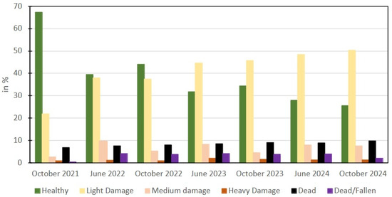
Figure 8.
Temporal evolution of tree categories.
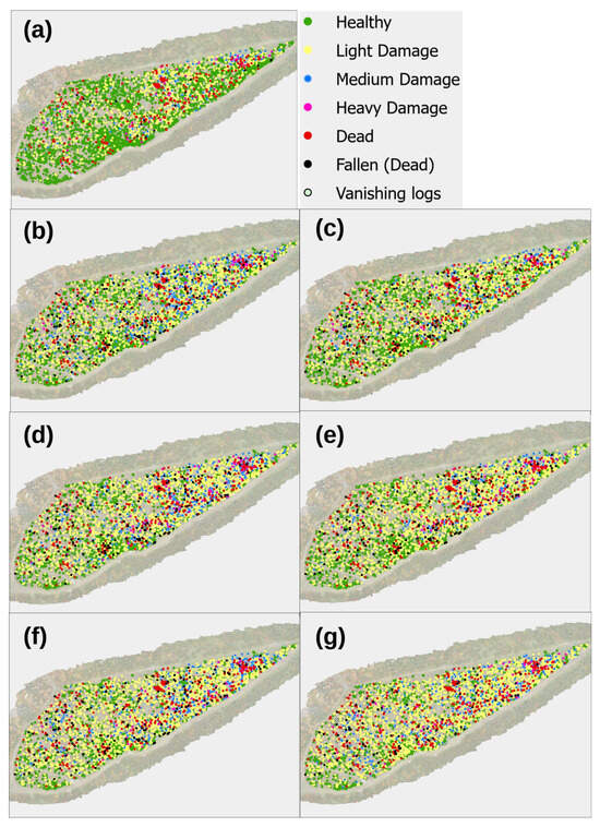
Figure 9.
Orthomosaics showing health status of trees across different time periods The orthomosaics illustrate the health status of trees in the study area, categorized as Healthy, Light Damage, Medium Damage, Heavy Damage, Dead, Fallen, or Vanishing Logs. Each map represents a specific time period: (a) October 2021, (b) June 2022, (c) October 2022, (d) June 2023, (e) October 2023, (f) June 2024, and (g) October 2024.
In the southwestern half of the area of site 2, a higher number of healthy trees was observed, whereas at higher elevations, particularly around site 5, more significant damage was observed. At sites 4 and 5, approximately 95% of the trees were dead. At site 2, two main hotspots with a higher concentration of dead trees were found, in the northeastern and the central part, while fallen trees were evenly distributed across the site. In October 2021, the proportion of healthy trees was highest at 2695 (67.4% trees). This figure dropped to 1120 trees (27.9%) by June 2024, reaching its lowest level of 1029 trees (25.6%) in October 2024. This indicates a continuous decline in the overall health of the forest. The sharpest decrease occurred between 2021 and 2022, with a drop from 2695 to 1580 trees (June 2022). The category “Light Damage” showed a steady increase over time. The proportion rose from 875 trees (21.9%) in October 2021 to 2024 trees (50.4%) in October 2024 (Table 3).
The most significant rise in tree damage occurred after June 2023, indicating increasing external stress factors. The proportion of trees with medium damage fluctuated over the observation period. It peaked at 9.5% (382 trees) in June 2022 and decreased to 4.6% (183 trees) in October 2023, while in October 2024, the proportion stood at 7.6% (307 trees). This suggests that medium-damage trees are less frequent but persist over time. Heavy Damage was the least frequent category but showed a slight increase from 0.9% (36 trees) in October 2021 to 1.2% (50 trees) in October 2024. A temporary rise to 2.0% (80 trees) in June 2023 could point to a specific stress factor during this period. The proportion of dead trees (Dead) rose from 6.9% (274 trees) in October 2021 to 9.8% (395 trees) in October 2024. The category “Fallen” showed a similar development, increasing from 0.4% (17 trees) in October 2021 to 2.0% (81 trees) in October 2023. Both categories, “Dead” and “Fallen”, reached their highest values in June 2023, with 342 dead and 167 fallen trees recorded. The most pronounced increase in fallen trees occurred between October 2021 (17 trees) and June 2022 (163 trees), indicating a particularly significant phase of tree fall within this period. The category “Vanishing Logs” was negligible until June 2022 (<0.5%) but increased to 3.3% (132 trees) by October 2024. This suggests that many of these trees had previously fallen and were now no longer visible in the orthomosaics.
For a simplified overview, the categories “Light Damage”, “Medium Damage”, and “Heavy Damage”, as well as “Dead” and “Fallen”, were combined to represent total non-healthy trees: October 2021: 1306 trees (32.6%), June 2022: 2427 trees (60.6%), October 2022: 2240 trees (55.9%), June 2023: 2779 trees (68.2%), October 2023: 2631 trees (65.6%), June 2024: 2888 trees (72.1%), October 2024: 2989 trees (74.4%). This trend highlights a clear increase in damaged and dead trees over time, while less than one-third of the trees were damaged or dead in 2021, by 2024, nearly three-quarters of the all trees were damaged or dead. The increase in the number of light-damage trees can be used an early indicator of deteriorating forest health (Figure 9 and Figure 10).
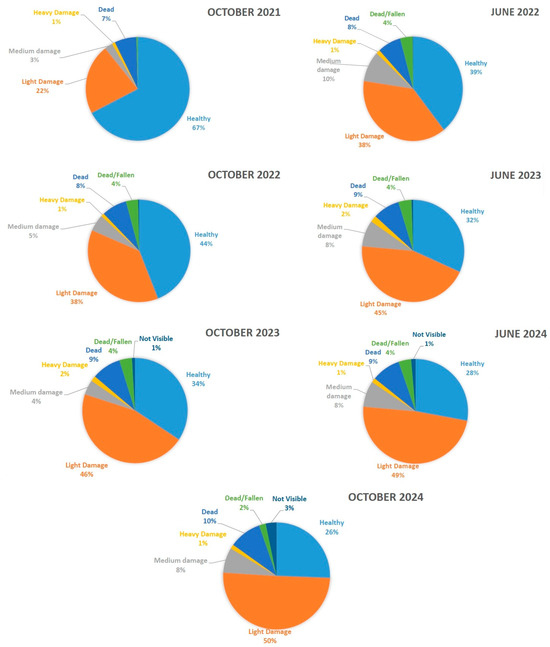
Figure 10.
Tree health temporal change from October 2021 to October 2024. Represented in the categories Healthy, Light Damage, Medium Damage, Heavy Damage, Dead, Fallen, and Vanishing Logs.
3.2. Deep Learning Networks to Automatically Predict Forest Health
The model was applied to the test area, and the figure shows a forest section from September 2024 with the YOLO model in operation. The results clearly demonstrate that the model works as intended, delivering accurate predictions and categorization (Figure 11). This confirms its functionality and highlights its effectiveness in practical use. The visualization serves as a concrete example of the model’s performance on real-world data (Figure 12).
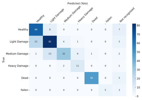
Figure 11.
Confusion matrix for true vs. YOLO classification.
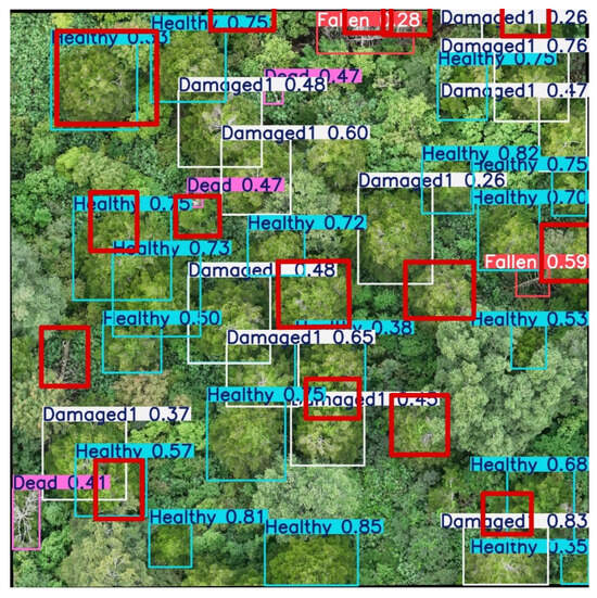
Figure 12.
Result of YOLO applied on the orthomosaic of September 2024.
The results of the classification model’s performance were analyzed and compared based on two different approaches: separated categories and aggregated categories. The model’s performance was assessed using key metrics, namely, accuracy, precision, recall, F1-score, and IoU (Equations (1)–(5)). The overall model accuracy was 74.9% for separated categories and was higher for aggregated categories at 82.8%.
3.3. Performance of Separated Categories
For the approach using separated categories, which includes the classes Healthy, Light Damage, Medium Damage, Heavy Damage, Dead, and Fallen, the model shows a more granular classification of the data. The Fallen category achieved perfect precision, scoring 100%, while the Dead category also performed well with a precision of 98.0%. The Heavy Damage category had the lowest precision, with a score of 64.7%. In terms of recall, the Dead category ranked the highest with 90.6%, followed by Heavy Damage at 78.6%. The Light Damage category had the lowest recall at 71.3%. The F1-score was highest for the Dead category with 94.1%, while the Fallen category achieved an F1-score of 76.9%. The Medium Damage category showed the lowest F1-score at 68.8%. In terms of IoU, the Dead category led with 88.9%, while the Heavy Damage category showed the lowest IoU at 54.6%. This approach provided more detailed insights into the model’s performance for specific classes, though some categories, particularly Heavy Damage and Medium Damage, showed lower performance compared to the aggregated categories (Table 4).
Table 4.
Performance metrics for separated categories based on the confusion matrix.
3.4. Performance of Aggregated Categories
The performance metrics for the aggregated categories, which include the classes Healthy, Damage, and Decay, showed the highest precision for the Decay category (98.2%), followed closely by the Damage category (94.9%), while the lowest precision was found for the Healthy category (73.3%). When evaluating recall, the Decay category shows the highest recall at 86.9%, followed by Damage at 81.9%, while the Healthy category achieves a recall of 81.5%. Regarding the F1-score, the Decay category performs best with a score of 92.1%, while Damage follows closely with 87.8%. The Healthy category has the lowest F1-score at 77.3%. Finally, in terms of IoU, the Decay category again leads with 85.6%, followed by Damage at 78.5%. The Healthy category exhibits the lowest IoU at 62.2%. These results suggest that the model excels in classifying the Damage and Decay categories, but the Healthy category experiences a notable drop in performance (Table 5).
Table 5.
Performance metrics for aggregated categories based on the confusion matrix.
3.5. Comparison of Aggregated and Separated Categories
A comparison between the aggregated and separated categories shows that the aggregated approach outperforms the separated approach in most metrics. The accuracy of the aggregated categories was 82.8%, compared to 74.9% for the separated categories. This indicates that the aggregated approach benefits from reduced complexity while maintaining a higher overall accuracy. For precision, the aggregated approach scored 82.1%, while the separated categories had a precision of 78.4%. This suggests that the aggregated model achieved better accuracy in classifying the Damage and Decay categories. The recall was slightly higher for the aggregated categories (81.3%) compared to the separated categories (80.2%). The F1-score was also higher for the aggregated categories at 80.7%, compared to 78.4% for the separated categories. Additionally, the IoU for the aggregated categories was 76.8%, whereas the separated categories achieved a lower IoU of 72.2% (Table 6).
Table 6.
Comparison of metrics for aggregated and separated categories.
3.6. Data Distribution and Challenges
The data distribution shows that 23 trees were not detected: 7 healthy, 5 light-damage, 2 medium-damage, 1 heavy-damage, 5 dead, and 3 fallen trees were not classified. Additionally, seven trees were detected twice, with the more accurate prediction being included in the confusion matrix and the incorrect one discarded (Figure 13). Among these duplicate detections, one tree had no true value, as the YOLO Medium Damage and Heavy Damage categories both failed to identify the tree correctly. Furthermore, two trees were falsely detected despite not existing: one in the Healthy category and one in the Dead category. These error sources underscore the challenges in classification, particularly for trees with ambiguous or fluid transitions between classes.
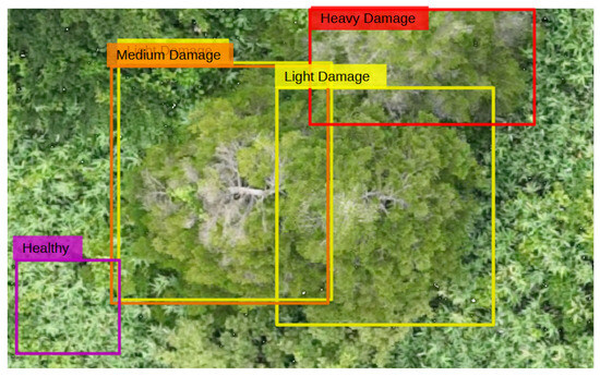
Figure 13.
Examples of YOLO detection challenges: double detection (yellow and orange overlapping) of one tree (Medium Damage is true category) and healthy tree identified without true data (violet).
Overall, the aggregated categories approach demonstrates superior performance in terms of accuracy, precision, F1-score, and IoU. This approach is advantageous when the categories can be grouped together without significant loss in classification quality, making it ideal for scenarios where simplicity and efficiency are key. In contrast, the separated categories approach provides more detailed insights into the performance of individual classes, which may be beneficial in applications requiring fine-grained classification. However, this approach comes with a trade-off, as it results in lower overall accuracy and precision for certain categories, such as Medium Damage and Heavy Damage. While the aggregated categories approach is more effective in general, the separated categories approach may still be useful in specific cases where detailed classification is essential. In summary, the model performs strongly in detecting decaying trees (Dead and Fallen categories), while the classification of Healthy and Damage category trees could be further optimized.
4. Discussion
In this study, we examined recent advances in model architectures, data pre-processing techniques, and validation strategies to improve detection accuracy and generalization. Many studies use test sets that are not truly independent [44,45]. Instead, the training and test data come from the same distribution, but differ in temporal characteristics, which can lead to overly optimistic performance estimates and reduce real-world applicability [45]. The comparison between separated and combined classes shows that the model is better at detecting and localizing damaged trees as a whole than at distinguishing between different levels of damage. The results shows that expanding the training dataset, particularly for the Light Damage and Fallen classes, and fine-tuning the model architecture would improve overall performance. This indicates that further differentiation of damage levels is needed in future work to enhance the model’s accuracy and robustness [46] (Table 4 and Table 5).
4.1. Discussion—Observed Spatial and Temporal Tree Health Patterns
Defoliation is a key indicator of tree health and decline, with various studies using different classification schemes to describe this progression [11,47]. While many studies categorize tree conditions based on color phases—typically progressing from green (healthy) to red (severely damaged) and eventually gray (dead), like in Safonova et al. 2019 [37] or Kapil et al. 2022 [39]—our study applies a classification system based on the degree of defoliation [11]. Specifically, we classify the trees into Healthy, Light Damage, Medium Damage, Heavy Damage, Dead, and Fallen groups. In contrast to studies that emphasize a red phase as an intermediate stage of heavy damage, our data suggest a direct transition from damaged states to the Dead or Fallen categories, with the red phase being rare or absent. This highlights differences in how tree decline manifests across different study systems and classification approaches. Another observation that deviates from our initial expectations is that a large number of trees remain stable or decline slowly over time after showing initial damage. Previous observations at site 5 showed that the bark beetle infestation progressed quickly, with a large tree mortality within a period of one to two years [6,41,48]. Despite these previous observations, we observe a clear increase from 875 to over 2000 in damaged trees but the proportion of dead trees remains stable at 8% to 10% (Figure 8). This indicates that tree mortality is not an immediate consequence of damage as many trees can persist in a weakened state for extended periods. The spatial distribution of damage progression also follows distinct patterns [49]. Site 5 exhibit similarities to site 4 and site 2 resembles site 3. However, since sites 3 and 4 have only been monitored for a shorter period, they are considered to a lesser extent in this study. One possible explanation for these patterns is the elevation range of the study area (1332 m to 1670 m). P. proximus has been recorded at elevations up to 1493 m a.s.l. in the Altai Republic, aligning with the upper limit of Siberian fir distribution [7,50]. Our study area, with an altitude up to 1670 m a.s.l., lies above this. At these elevations, bark beetle outbreaks may be naturally constrained by the upper elevation limit of P. proximus, reducing the likelihood of sustained infestations. Instead, severe but short-lived disturbances—-including a severe E. piceae moth infestation in 2012—may create ideal conditions for bark beetle outbreaks, which might only occur under optimal conditions, such as in 2013, when a combination of factors facilitated their proliferation [3,51]. Furthermore, the climatic conditions of the study area are related to bark beetle activity and are likely to be one of its main drivers [3,7,50]. While it is not possible to rigorously ascertain the extent of this impact without a deeper and much longer entomological study, some possible explanations follow: Snow cover persists well into spring, delaying the onset of the growing season. Although summer temperatures are relatively mild (16–19 °C), the short vegetation period may hinder the development of frequent, large-scale outbreaks. This may explain why many damaged trees persist for extended periods rather than transitioning rapidly to mortality. As a side note, the number of trees classified as “Vanishing Logs” has increased over time, mostly due to fallen trees decomposing or becoming overgrown by surrounding vegetation, making them undetectable in the orthomosaics.
Overall, it becomes apparent that the expansion of areas with a high proportion of at least lightly damaged trees initially occurs more prominently at higher elevations. However, over the years, these damaged areas gradually expand to lower parts of the study area. In particular, to so-called hotspots, small areas within the study site with a high density of dead trees and trees affected by heavy damage. Nevertheless, the general movement from higher to lower elevations remains clearly recognizable. In contrast, fallen trees, as well as vanishing logs, appear to be distributed irregularly across the study area without a direct spatial connection to the hotspots mentioned above. It is also noticeable that many of the fallen trees were classified as healthy in the previous years, especially between 2021 and 2022. This indicates that these occurrences are not primarily the result of bark beetle infestation but are more likely caused by external factors such as extreme weather events. Given the high number of already damaged trees and the observed trends, it is likely that the proportion of severely damaged and dead trees will continue to increase in the coming years. However, the rate and extent of this transition remains uncertain, emphasizing the need for long-term monitoring to better understand the forest response to extreme environmental factors [3,41].
4.2. Discussion—Performance of the YOLO Deep Learning Model
The presented results illustrate the performance of the model in categorizing forest conditions based on RGB imagery. The analysis includes both separated and aggregated category definitions to explore the model strengths and limitations under varying classification schemes. It is important to note that the model was trained using RGB data, with defoliation serving as the primary visual cue for distinguishing between tree health categories. In addition, the model was evaluated on data from different time periods than those used for training, providing an assessment of its generalization capabilities under realistic conditions. The results for aggregated categories (Table 5) indicate a high classification performance for clearly distinguished categories. The Decay category, which combines Dead and Fallen trees, achieved an F1-score of 92.1% and an IoU of 85.6%. Similarly, the Damage category, encompassing all levels of visible defoliation, achieved strong performance values. These findings demonstrate the model’s robustness in detecting the substantial degradation in the forest ecosystem. In contrast, the analysis of separated categories (Table 4) reveals certain challenges. While the model achieved high precision for Dead and Fallen trees, the results for the Healthy and Light Damage categories showed low precision and increased misclassification. In particular, tress in the Healthy category were occasionally classified in the Light Damage category, which may be attributed to subtle visual similarities. Since the model relies on defoliation as the main indicator, natural variations in crown density or illumination effects can lead to confusion between these two categories. Additionally, the defoliation associated with the Light Damage class is often mild and difficult to distinguish in RGB imagery, further contributing to classification uncertainty. The Fallen category also presents an interesting case. Although it achieved a precision of 100%, the recall was limited to 62.5%. This suggests that while positively identified fallen trees are reliable, a significant portion remains undetected. This could be due to overgrown vegetation, different defoliation levels, and the shape of fallen trees, which differ substantially from the vertical structure of standing trees and may not always be captured clearly in imagery. A comparison of the average metrics (Table 6) shows that the use of aggregated categories consistently improves model performance. Accuracy (82.8% vs. 74.9%) and F1-score (80.7% vs. 78.4%) were higher in the aggregated classification, reflecting a reduction in intra-category confusion. These results suggest that while the model is generally capable of distinguishing between healthy and unhealthy trees, it is less effective at differentiating between degrees of damage. The high intra-category variability and the gradual transitions between light, medium, and heavy damage contribute to this limitation. At the same time, the detailed classification provides deeper insight into the progression of damage, which is critical for understanding long-term forest health trends [52,53]. The combined use of both metrics enhances the interpretability of the model’s predictions, offering a balance between accuracy and detailed insight, making them adaptable to different monitoring needs depending on the specific requirements of the use case. Ultimately, the results highlight the importance of accurately distinguishing between damaged, dead, and fallen trees, as each category demands different management practice. The potential of the model to detect these transitions with a high degree of confidence strengthens its utility for automated forest monitoring. Moreover, the use of independent and highly variable test data underscores the robustness of the evaluation, demonstrating that the model can perform well across different conditions rather than being limited to a specific dataset. This enhances confidence in its application for large-scale, long-term forest health assessments. Overall, the findings highlight the strengths of RGB-based tree classification for health assessments. The model performs particularly well in detecting clearly defined conditions such as full defoliation (Dead class) or the absence of a tree (Fallen class). However, it struggles to capture more subtle transitions in foliage density. For future applications, a bigger and more diverse dataset could enhance the detection of nuanced canopy conditions. In practice, the level of health category detail should be aligned with the application context. Aggregated classes appear to offer a more robust and comprehensible solution for large-scale monitoring, while fine-grained category definitions may provide additional ecological insights at the cost of classification certainty. Balancing model complexity, data quality, and application-specific requirements remains a key consideration for operational deployment. It should be noted, however, that this study is one of the few that applies such a complex and detailed classification approach at the level of individual trees. Most recent studies, such as those by Kerchev et al. 2024, Illarionova et al. 2024, Anwander et al. 2024, or Safonova et al. 2022 [26,27,28,29], typically use between one and four categories for damage classification. For example, Tan et al. 2024 [30] applied a four-class system (from Green Stage to White Stage) and reported an overall precision of 0.64 and a recall of 0.58. Other studies provide more detailed class-specific results. Kanerva et al. 2022 [31], for instance, used three classes (Healthy, Infested, Dead), with precision values ranging from 10.5% to 96%, and recall values between 25% and 100%, depending on the class. Further studies, such as Zhu et al. 2024 [32], Wang et al. 2024 [21], and Ma et al. 2025 [33], used only single or binary classification (dead or not healthy), reporting precision values between 67% and 90%, and recall values between 69% and 90%. A key factor contributing to the robustness of the model evaluation is the diversity of our dataset, especially its temporal aspect and varying conditions. By ensuring that the trees in the test set were captured at a different time than those in the training and validation sets, we replicate the expected use-case conditions for assessing the progression of infestations. This approach reflects the practical scenario of monitoring infestation evolution over time. It is important to note that while the test set contains the same trees as the training and validation sets, they were captured at different times, as described in the methodology, in order to make the model able to detect tree healthy temporal variability. Thus, the test data were not used for model training and originate from different time periods, making them temporally independent from the training distribution. It is essential to evaluate models in conditions that closely mirror real-world use cases in order to truly ensure their robustness [45]. While our model has not been tested in other regions or environments, it would be valuable if it could be deployed in different settings. Fir forests (containing four different fir species) are spread from Gifu Prefecture in the south to Aomori Prefecture in the north of Honshu Island in Japan [48].
5. Conclusions
The results demonstrate that the combination of high-resolution RGB imagery and DL models is an effective tool for categorization of tree health conditions. With the help of UAVs, we were able to track the progression of forests in the Zao Mountains in high detail over a period of four years. Moreover, DL allowed for the analysis of larger areas in shorter time frames, making the combination of UAVs and DL highly scalable for monitoring vast regions. The model achieved an accuracy of 71.4% and highlights the potential of this technology. However, challenges remain, particularly in distinguishing between healthy trees and those with light damage, as well as among the various damage level categories (Light Damage, Medium Damage, Heavy Damage). Many of the misclassifications occurred at the boundary areas between categories, where the transitions between defoliation categories were gradual, making precise classification difficult due to less distinct features in these regions. The spatial and temporal analysis of tree health revealed a continuous decline in healthy trees, from 67.4% in October 2021 to 25.6% in October 2024. Simultaneously, the proportion of damaged and dead trees increased from 32.6% to 74.4% over the same period. This trend underscores the severe impact of bark beetle infestations and the ongoing deterioration of forest health.
The DL models showed high accuracy, highlighting the ability of the model for reliably detection. Aggregating the damage categories into a single category (Damage) improved the model performance, indicating that distinguishing between damage levels needs still more work. The discrepancies between the true data (330 trees) and YOLO detections (344 trees) point to detection issues, such as overlapping features, doubly detected trees, or prediction errors. These discrepancies emphasize the need for further improvements. Future work should focus on enhancing feature extraction, improving data quality, and accounting for environmental factors that influence tree health. These insights can serve as a base for targeted management measures to enhance forest monitoring and improve resilience against future disturbances.
Author Contributions
Conceptualization, T.L.; methodology, T.L.; software, T.L.; validation, T.L.; formal analysis, T.L.; investigation, T.L.; resources, T.L.; data curation, T.L.; writing—original draft preparation, T.L.; writing—review and editing, M.L.L.C., C.F., Y.D., C.-Y.T. and M.K.; visualization, T.L.; supervision, M.L.L.C.; project administration, M.L.L.C.; funding acquisition, M.L.L.C. All authors have read and agreed to the published version of the manuscript.
Funding
This research received no external funding.
Data Availability Statement
The data supporting the findings of this study are available from the corresponding author upon reasonable request at the time of publication.
Conflicts of Interest
The authors declare no conflicts of interest.
Abbreviations
The following abbreviations are used in this manuscript:
| DL | Deep learning |
| px | Pixel |
| Yolo | You Only Look Once |
| TP | True positive |
| TN | True negative |
| FP | False positive |
| FN | False negative |
| GCPs | Ground control points |
References
- Guégan, J.F.; Thoisy, B.; Gómez-Gallego, M.; Jactel, H. World forests, global change, and emerging pests and pathogens. Curr. Opin. Environ. Sustain. 2023, 61, 101266. [Google Scholar] [CrossRef]
- Jactel, H.; Castagneyrol, B. Responses of forest insect pests to climate change: Not so simple. Curr. Opin. Insect Sci. 2019, 35, 103–108. [Google Scholar] [CrossRef] [PubMed]
- Singh, V.; Naseer, A.; Mogilicherla, K.; Trubin, A.; Zabihi, K.; Roy, A.; Jakuš, R.; Erbilgin, N. Understanding bark beetle outbreaks: Exploring the impact of changing temperature regimes, droughts, forest structure, and prospects for future forest pest management. Rev. Environ. Sci. Biotechnol. 2024, 23, 257–290. [Google Scholar] [CrossRef]
- Bonan, G.B. Forests and Climate Change: Forcings, Feedbacks, and the Climate Benefits of Forests. Science 2008, 320, 1444–1449. [Google Scholar] [CrossRef] [PubMed]
- Fassnacht, F.E.; Latifi, H.; Ghosh, A.; Joshi, P.K.; Koch, B. Assessing the potential of hyperspectral imagery to map bark beetle-induced tree mortality. Remote Sens. Environ. 2014, 140, 533–548. [Google Scholar] [CrossRef]
- Kloucek, T.; Komárek, J.; Surový, P.; Hrach, K.; Janata, P.; Vašícek, B. The Use of UAV Mounted Sensors for Precise Detection of Bark Beetle Infestation. Remote Sens. 2019, 11, 1561. [Google Scholar] [CrossRef]
- EPPO. EPPO Global Database. Datasheet: Polygraphus proximus. 2025. Available online: https://gd.eppo.int/taxon/POLGPR (accessed on 26 February 2025).
- Schroeder, L.; Weslien, J.; Åke, L.; Lindhe, A. Attacks by bark- and wood-boring Coleoptera on mechanically created high stumps of Norway spruce in the two years following cutting. For. Ecol. Manag. 1999, 123, 21–30. [Google Scholar] [CrossRef]
- Jaime, L.; Batllori, E.; Lloret, F. Bark beetle outbreaks in coniferous forests: A review of climate change effects. Eur. J. For. Res. 2024, 143, 1–17. [Google Scholar] [CrossRef]
- Müller, J.; Bußler, H.; Goßner, M.; Rettelbach, T.; Duelli, P. The European spruce bark beetle Ips typographus in a national park: From pest to keystone species. Biodivers. Conserv. 2008, 17, 2979–3001. [Google Scholar] [CrossRef]
- Leidemer, T.; Gonroudobou, O.; Nguyen, H.; Ferracini, C.; Burkhard, B.; Diez, Y.; Lopez Caceres, M. Classifying the Degree of Bark Beetle-Induced Damage on Fir (Abies mariesii) Forests, from UAV-Acquired RGB Images. Computation 2022, 10, 63. [Google Scholar] [CrossRef]
- Ecke, S.; Dempewolf, J.; Frey, J.; Schwaller, A.; Endres, E.; Klemmt, H.J.; Tiede, D.; Seifert, T. UAV-Based Forest Health Monitoring: A Systematic Review. Remote Sens. 2022, 14, 3205. [Google Scholar] [CrossRef]
- Näsi, R.; Honkavaara, E.; Lyytikäinen-Saarenmaa, P.; Blomqvist, M.; Litkey, P.; Hakala, T.; Viljanen, N.; Kantola, T.; Tanhuanpää, T.; Holopainen, M. Using UAV-Based Photogrammetry and Hyperspectral Imaging for Mapping Bark Beetle Damage at Tree-Level. Remote Sens. 2015, 7, 15467–15493. [Google Scholar] [CrossRef]
- Capolupo, A.; Kooistra, L.; Berendonk, C.; Boccia, L.; Suomalainen, J. Estimating Plant Traits of Grasslands from UAV-Acquired Hyperspectral Images: A Comparison of Statistical Approaches. Isprs Int. J. Geo-Inf. 2015, 4, 2792–2820. [Google Scholar] [CrossRef]
- Tran, T.; Lopez Caceres, M.; Riera, S.i.; Conciatori, M.; Kuwabara, Y.; Tsou, C.Y.; Diez, Y. Using UAV RGB Images for Assessing Tree Species Diversity in Elevation Gradient of Zao Mountains. Remote Sens. 2024, 16, 3831. [Google Scholar] [CrossRef]
- Gambella, F.; Sistu, L.; Piccirilli, D.; Corposanto, S.; Caria, M.; Arcangeletti, E.; Proto, A.R.; Chessa, G.; Pazzona, A. Forest and UAV: A Bibliometric Review. Contemp. Eng. Sci. 2016, 9, 1359–1370. [Google Scholar] [CrossRef]
- Paneque-Gálvez, J.; McCall, M.; Napoletano, B.; Wich, S.; Koh, L. Small Drones for Community-Based Forest Monitoring: An Assessment of Their Feasibility and Potential in Tropical Areas. Forests 2014, 5, 1481–1507. [Google Scholar] [CrossRef]
- Gonroudobou, O.B.H.; Silvestre, L.H.; Diez, Y.; Nguyen, H.T.; Caceres, M.L.L. Treetop Detection in Mountainous Forests Using UAV Terrain Awareness Function. Computation 2022, 10, 90. [Google Scholar] [CrossRef]
- Mohan, M.; Richardson, G.; Gopan, G.; Aghai, M.M.; Bajaj, S.; Galgamuwa, G.A.P.; Vastaranta, M.; Arachchige, P.S.P.; Amorós, L.; Corte, A.P.D.; et al. UAV-Supported Forest Regeneration: Current Trends, Challenges and Implications. Remote Sens. 2021, 13, 2596. [Google Scholar] [CrossRef]
- Reichstein, M.; Camps-Valls, G.; Stevens, B.; Jung, M.; Denzler, J.; Carvalhais, N.; Prabhat, F. Deep learning and process understanding for data-driven Earth system science. Nature 2019, 566, 195–204. [Google Scholar] [CrossRef]
- Wang, L.; Cai, J.; Wang, T.; Zhao, J.; Gadekallu, T.R.; Fang, K. Detection of Pine Wilt Disease Using AAV Remote Sensing with an Improved YOLO Model. IEEE J. Sel. Top. Appl. Earth Obs. Remote Sens. 2024, 17, 19230–19242. [Google Scholar] [CrossRef]
- Yu, R.; Luo, Y.; Zhou, Q.; Zhang, X.; Wu, D.; Ren, L. Early detection of pine wilt disease using deep learning algorithms and UAV-based multispectral imagery. For. Ecol. Manag. 2021, 497, 119493. [Google Scholar] [CrossRef]
- Gensheng, H.; Pan, Y.; Mingzhu, W.; Wenxia, B.; Weihui, Z. Detection and classification of diseased pine trees with different levels of severity from UAV remote sensing images. Ecol. Inform. 2022, 72, 101844. [Google Scholar]
- Jarahizadeh, S.; Salehi, B. Advancing tree detection in forest environments: A deep learning object detector approach with UAV LiDAR data. Urban For. Urban Green. 2025, 105, 128695. [Google Scholar] [CrossRef]
- Zhou, Y.; Liu, W.; Bi, H.; Chen, R.; Zong, S.; Luo, Y. A Detection Method for Individual Infected Pine Trees with Pine Wilt Disease Based on Deep Learning. Forests 2022, 13, 1880. [Google Scholar] [CrossRef]
- Kerchev, I.; Markov, N.; Machuca, C.; Tokareva, O. Classification of pest-damaged coniferous trees in unmanned aerial vehicles images using convolutional neural network models. Comput. Res. Model. 2024, 16, 1271–1294. [Google Scholar] [CrossRef]
- Illarionova, S.; Tregubova, P.; Shukhratov, I.; Shadrin, D.; Kedrov, A.; Burnaev, E. Remote sensing data fusion approach for estimating forest degradation: A case study of boreal forests damaged by Polygraphus proximus. Front. Environ. Sci. 2024, 12, 1412870. [Google Scholar] [CrossRef]
- Anwander, J.; Brandmeier, M.; Paczkowski, S.; Neubert, T.; Paczkowska, M. Evaluating Different Deep Learning Approaches for Tree Health Classification Using High-Resolution Multispectral UAV Data in the Black Forest, Harz Region, and Göttinger Forest. Remote Sens. 2024, 16, 561. [Google Scholar] [CrossRef]
- Safonova, A.; Hamad, Y.; Alekhina, A.; Kaplun, D. Detection of Norway Spruce Trees (Picea Abies) Infested by Bark Beetle in UAV Images Using YOLOs Architectures. IEEE Access 2022, 10, 10384–10392. [Google Scholar] [CrossRef]
- Tan, C.; Lin, Q.; Du, H.; Chen, C.; Hu, M.; Chen, J.; Huang, Z.; Xu, Y. Detection of the Infection Stage of Pine Wilt Disease and Spread Distance Using Monthly UAV-Based Imagery and a Deep Learning Approach. Remote Sens. 2024, 16, 364. [Google Scholar] [CrossRef]
- Kanerva, H.; Honkavaara, E.; Näsi, R.; Hakala, T.; Junttila, S.; Karila, K.; Koivumäki, N.; Alves Oliveira, R.; Pelto-Arvo, M.; Pölönen, I.; et al. Estimating Tree Health Decline Caused by Ips typographus L. from UAS RGB Images Using a Deep One-Stage Object Detection Neural Network. Remote Sens. 2022, 14, 6257. [Google Scholar] [CrossRef]
- Zhu, X.; Wang, R.; Shi, W.; Liu, X.; Ren, Y.; Xu, S.; Wang, X. Detection of Pine-Wilt-Disease-Affected Trees Based on Improved YOLO v7. Forests 2024, 15, 691. [Google Scholar] [CrossRef]
- Ma, H.; Yang, B.; Wang, R.; Yu, Q.; Yang, Y.; Wei, J. Automatic Extraction of Discolored Tree Crowns Based on an Improved Faster-RCNN Algorithm. Forests 2025, 16, 382. [Google Scholar] [CrossRef]
- Andresini, G.; Appice, A.; Ienco, D.; Recchia, V. DIAMANTE: A data-centric semantic segmentation approach to map tree dieback induced by bark beetle infestations via satellite images. J. Intell. Inf. Syst. 2024, 62, 1531–1558. [Google Scholar] [CrossRef]
- Crosby, M.K.; McConnell, T.E.; Holderieath, J.J.; Meeker, J.R.; Steiner, C.A.; Strom, B.L.; Johnson, C.W. The Use of High-Resolution Satellite Imagery to Determine the Status of a Large-Scale Outbreak of Southern Pine Beetle. Remote Sens. 2024, 16, 582. [Google Scholar] [CrossRef]
- Minařík, R.; Langhammer, J.; Lendzioch, T. Detection of Bark Beetle Disturbance at Tree Level Using UAS Multispectral Imagery and Deep Learning. Remote Sens. 2021, 13, 4768. [Google Scholar] [CrossRef]
- Safonova, A.; Tabik, S.; Alcaraz-Segura, D.; Rubtsov, A.; Maglinets, Y.; Herrera, F. Detection of Fir Trees (Abies sibirica) Damaged by the Bark Beetle in Unmanned Aerial Vehicle Images with Deep Learning. Remote Sens. 2019, 11, 643. [Google Scholar] [CrossRef]
- Zhang, J.; Cong, S.; Zhang, G.; Ma, Y.; Zhang, Y.; Huang, J. Detecting Pest-Infested Forest Damage through Multispectral Satellite Imagery and Improved UNet++. Sensors 2022, 22, 7440. [Google Scholar] [CrossRef]
- Kapil, R.; Marvasti-Zadeh, S.M.; Goodsman, D.; Ray, N.; Erbilgin, N. Classification of Bark Beetle-Induced Forest Tree Mortality using Deep Learning. arXiv 2022, arXiv:2207.07241. [Google Scholar] [CrossRef]
- Bright, B.C.; Hudak, A.T.; Kennedy, R.E.; Meddens, A.J.H. Landsat Time Series and Lidar as Predictors of Live and Dead Basal Area Across Five Bark Beetle-Affected Forests. IEEE J. Sel. Top. Appl. Earth Obs. Remote Sens. 2014, 7, 3440–3452. [Google Scholar] [CrossRef]
- Chiba, S.; Shotaro, K.; Kosuke, H. Wide-area assessment of mass mortality in Abies mariesii forests in the Zao mountain range and subsequent regeneration. J. Jpn. For. Soc. 2020, 102, 108–114. [Google Scholar] [CrossRef]
- Redmon, J.; Farhadi, A. YOLO9000: Better, Faster, Stronger. arXiv 2016, arXiv:1612.08242. [Google Scholar] [CrossRef]
- Redmon, J.; Divvala, S.; Girshick, R.; Farhadi, A. You Only Look Once: Unified, Real-Time Object Detection. Remote Comput. Vis. Found. 2016, 779–788. [Google Scholar] [CrossRef]
- Genest, C.; Nešlehová, J.; Remillard, B.; Murphy, O. Testing for independence in arbitrary distributions. Biometrika 2019, 106, 47–68. [Google Scholar] [CrossRef]
- Diez, Y.; Kentsch, S.; Fukuda, M.; Caceres, M.L.L.; Moritake, K.; Cabezas, M. Deep Learning in Forestry Using UAV-Acquired RGB Data: A Practical Review. Remote Sens. 2021, 13, 2837. [Google Scholar] [CrossRef]
- Tae, K.; Roh, Y.; Oh, Y.; Kim, H.; Whang, S. Data Cleaning for Accurate, Fair, and Robust Models: A Big Data—AI Integration Approach. In Proceedings of the 3rd International Workshop on Data Management for End-to-End Machine Learning, Amsterdam, The Netherlands, 30 June 2019; pp. 1–4. [Google Scholar] [CrossRef]
- Bussotti, F.; Potočić, N.; Timmermann, V.; Lehmann, M.M.; Pollastrini, M. Tree crown defoliation in forest monitoring: Concepts, findings, and new perspectives for a physiological approach in the face of climate change. For. Int. J. For. Res. 2024, 97, 194–212. [Google Scholar] [CrossRef]
- Tanaka, N.; Nakao, K.; Tsuyama, I.; Higa, M.; Nakazono, E.; Matsui, T. Predicting the impact of climate change on potential habitats of fir (Abies) species in Japan and on the East Asian continent. Procedia Environ. Sci. 2012, 13, 455–466. [Google Scholar] [CrossRef]
- Avila-Pérez, H.; Guzmán-Martínez, M.; Rosas-Acevedo, J.L.; Navarro-Martínez, J.; Gallardo-Bernal, I. Study of the Spatial Distribution of the Bark Beetle in the Ejido Tixtlancingo. Forests 2024, 15, 916. [Google Scholar] [CrossRef]
- Kerchev, I. Ecology of four-eyed fir bark beetle Polygraphus proximus Blandford (Coleoptera; Curculionidae, Scolytinae) in the west Siberian region of invasion. Russ. J. Biol. Invasions 2014, 5, 176–185. [Google Scholar] [CrossRef]
- Tello, M.; Tomalak, M.; Siwecki, R.; Gaper, J.; Motta, E.; Mateo-Sagasta, E. Biotic Urban Growing Conditions—Threats, Pests and Diseases. In Urban Forests and Trees: A Reference Book; Springer: Berlin/Heidelberg, Germany, 2005; pp. 325–365. [Google Scholar] [CrossRef]
- Acosta-Muñoz, C.; Navarro-Cerrillo, R.M.; Bonet-García, F.J.; Ruiz-Gómez, F.J.; González-Moreno, P. Evolution and Paradigm Shift in Forest Health Research: A Review of Global Trends and Knowledge Gaps. Forests 2024, 15, 1279. [Google Scholar] [CrossRef]
- Ciriani, M.L.; Dalstein, L. Forest Health Monitoring Highlights Progress in Forest Deterioration in France. Water Air Soil Pollut. 2018, 229. [Google Scholar] [CrossRef]
Disclaimer/Publisher’s Note: The statements, opinions and data contained in all publications are solely those of the individual author(s) and contributor(s) and not of MDPI and/or the editor(s). MDPI and/or the editor(s) disclaim responsibility for any injury to people or property resulting from any ideas, methods, instructions or products referred to in the content. |
© 2025 by the authors. Licensee MDPI, Basel, Switzerland. This article is an open access article distributed under the terms and conditions of the Creative Commons Attribution (CC BY) license (https://creativecommons.org/licenses/by/4.0/).