Drone-Enabled 3D Magnetometric Resistivity Imaging for Geological Hazard Detection: A Feasibility Study of Mapping Fracture Zones

Abstract

This study proposes a novel drone-based semi-airborne total-field magnetometric resistivity (SA-TFMMR) system for high-resolution detection of conductive fracture zones in geologically hazardous terrains. The system integrates a high-power, low-frequency grounded-wire transmitter with a drone-mounted total-field magnetometer, achieving high survey efficiency and extensive data coverage in mountainous areas. We develop a 3D inversion framework incorporating terrain-adaptive depth weighting, which successfully images a dipping water-saturated fracture zone model beneath a reservoir overburden at a tunnel water gushing accident site. Sensitivity analyses of SA-TFMMR reveal that the effectiveness of detection is controlled by the source-target coupling and the orientation of the target body with respect to the geomagnetic field. Optimal current injection along target strike directions amplifies magnetic anomalies, and orthogonal multi-source configurations can enhance imaging resolution. This UAV-geophysical integration provides a paradigm for pre-disaster monitoring of water-related geohazards.

1. Introduction

The deployment of uncrewed aerial vehicles (UAVs) in geophysical exploration has emerged as a transformative approach to survey hazardous or inaccessible terrains [1], such as integrating UAV-borne magnetometry, which has demonstrated successful applications in the near-surface detection of buried metallic objects [2,3], mineral exploration [4,5,6], and archaeological investigations of cultural relics [7]. While traditional ground-based methods such as DC resistivity and audio-frequency magnetotellurics (AMT) achieve high resolution in controlled environments [8,9,10,11,12,13], their reliance on surface electrode deployment renders them ineffective in steep mountainous regions, glacial areas, and swampy terrains, particularly in areas obscured by conductive overburdens such as swamps or water reservoirs, where electromagnetic (EM) signals experience severe attenuation. These limitations not only compromise spatial data coverage but also increase the risk of overlooking critical subsurface anomalies.

Semi-airborne geophysical systems, which synergize ground-based transmitters with UAV-borne receivers, offer a promising alternative to overcome topographic constraints [14]. Unlike conventional airborne electromagnetic (AEM) methods requiring large aircraft [15,16,17,18], these systems leverage the agility of drones to acquire data in logistically challenging areas [19,20]. Notable implementations include UAV-borne semi-airborne transient electromagnetic surveys for tunnel construction [21] and UAV-mounted systems for mining cavity detection [22]. However, a fundamental challenge persists: the induction coils used in these systems are inherently susceptible to motion-induced noise during UAV flights while cultural interference near survey areas further degrades data quality [23,24].

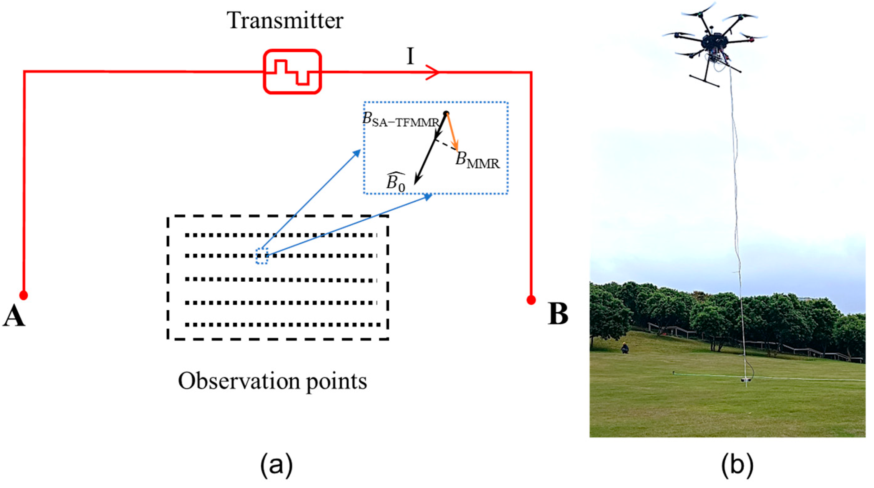
To address these limitations, this study introduces a novel drone-centric methodology: the semi-airborne total-field magnetometric resistivity (SA-TFMMR) system. By replacing induction coils with high-precision total-field magnetometers, a configuration analogous to the helicopter subaudio magnetic (HeliSAM) system [25], SA-TFMMR circumvents the motion noise plaguing traditional electromagnetic approaches; by utilizing grounded electrical sources to transmit low-frequency signals, it mitigates electromagnetic shielding and attenuation effects induced by low-resistivity overburdens overlying target anomalies. Traditional MMR techniques, predominantly applied to mineral and groundwater exploration in flat terrains [26,27,28,29,30,31,32], lack the capability to resolve depth-dependent structures in topographically complex regions. Our innovation lies in the integration of digital elevation models (DEMs) or on-site UAV-derived topographic data into a 3D inversion framework, enabling the reconstruction of geometrically intricate subsurface targets.

The SA-TFMMR framework advances UAV geophysics through two pivotal contributions. First, it establishes a robust 3D inversion algorithm that explicitly incorporates digital elevation models (DEMs), addressing the need for reliable detection of water-saturated fracture zones—key triggers of landslides and tunnel engineering hazards in geohazard-prone areas. Second, systematic investigations of electrode configurations and operational parameters provide actionable guidelines for field deployments, particularly in scenarios where conductive overburdens obscure deep anomalies. The methodology’s efficacy is demonstrated through synthetic models and a feasibility study, confirming its potential to bridge the gap between drone-based data acquisition and geologically meaningful subsurface characterization.

2. Method

2.1. Magnetometric Resistivity Method

The SA-TFMMR method is an electromagnetic exploration technique that combines ground-based DC/low-frequency current sources with drone-borne high-precision magnetometers to infer underground resistivity structures by measuring the spatial distribution of magnetic fields generated by subsurface currents [33]. In a typical MMR configuration (Figure 1), the current electrodes A and B are positioned at opposing sides of the survey region. The transmitter generates a steady-state current I. B_cable is the magnetic field produced by the cables on the ground connecting the transmitter and the electrodes. To minimize the effect of B_cable, the cables are placed as far from the measurement area as possible [34,35]. The direction of B_cable primarily contains a vertical component within the survey area. B_MMR is the secondary magnetic field generated by the current flowing underground and can be oriented in any direction depending on the subsurface conductivity structure. The data recorded by an MMR instrument are the sum of B_cable and B_MMR.

The SA-TFMMR and the MMR are fundamentally the same in the physical mechanism. Both techniques can be described using the modified Biot-Savart law

$${\mathit{B}}_{MMR}={\displaystyle \frac{\mu }{4\pi }}{\int }_v{\displaystyle \frac{{\nabla }^{’}U\left(r^{’}\right)\times {\nabla }^{’}\sigma \left(r^{’}\right)}{|r-r^{’}|}}d{v}^{’}$$

(1)

where $|r-r^{’}|$ is the distance between the observation point and the discretized volumetric element, and the direction of the magnetic field generated by the underground conductive current is determined by ${\nabla }^{’}U\left(r^{’}\right)\times {\nabla }^{’}\sigma \left(r^{’}\right)$. This magnetic field is highly sensitive to the gradients in conductivity distribution [36,37,38].

The main difference between these two techniques is that SA-TFMMR utilizes a total field magnetometer to measure the total magnetic field value (scalar) in the air rather than the three components or horizontal components (vector) of the magnetic field on the surface.

2.2. Forward Modeling

Many numerical approaches are available for the simulation of MMR responses [39,40,41,42,43]. Weng uses the frequency-domain Maxwell’s equations to establish a mathematical relation between the surface magnetic field and conductivity [44]. Jessop uses finite element or finite difference methods to calculate current density distribution and then generate observed magnetic field components using Biot-Savart law [36].

Our SA-TFMMR modeling algorithm is similar to Jessop and consists of two steps. First, we use the equivalent resistor network (RESnet) method to solve a 3D DC problem on a 3D rectilinear mesh [45]; the solution of the 3D DC problem provides the current intensities on all the edges of the mesh. In RESnet, the electric potential is defined at each node, and the discrete governing equations can be formulated using Kirchhoff’s Current Law (KCL)

$$-{\mathit{D}}^{\mathit{T}}diag\left(\mathit{g}\right)\mathit{D}\mathit{u}=-{\mathit{D}}^{\mathit{T}}diag\left(\mathit{G}·\mathit{\sigma }\right)\mathit{D}\mathit{u}=A\left(\mathit{\sigma }\right)\mathit{u}=\mathit{s}$$

(2)

where D is a sparse difference matrix containing only +1 or −1; u is the electric potential vector; s is the current source vector. RESnet efficiently models thin and highly conductive objects by defining integrated conductivity properties on mesh edges and faces, so the model parameter vector σ = (${\mathbf{\sigma }}_c$, ${\tilde{\mathbf{\sigma }}}_f$, ${\tilde{\mathbf{\sigma }}}_e$)^T is the stack of cell conductivity vector for volumetric objects, face conductivity vector for sheet-like objects (e.g., fractures) and edge conductivity for line objects (e.g., steel pipes). Generally, σ_c is non-zero, while ${\tilde{\mathbf{\sigma }}}_f$ and ${\tilde{\mathbf{\sigma }}}_e$ are mostly zero except for the mesh faces and edges that collocate with thin conductors. In Equation (2), the transformation matrix

$$\mathit{G}=\left[\begin{array}{ccc}{\mathit{G}}_{\mathit{c}}& & \\ & {\mathit{G}}_{\mathit{f}}& \\ & & {\mathit{G}}_{\mathit{e}}\end{array}\right]$$

(3)

converts the cell, surface, and edge conductivity parameters to the conductance on each branch of an equivalent resistor network. The current on each branch is then calculated using

$$\mathit{I}=diag\left(\mathit{G}·\mathit{\sigma }\right)\mathit{D}\mathit{u}$$

(4)

Next, the vector magnetic field at each observation point can be obtained by summing up the contributions from all the branch currents. The magnetic field due to a piece of finite-length current segment can be calculated using the Biot-Savart law. Because the current intensities defined on mesh edges can be approximated by a small piece of straight wire, the Biot-Savart law for the magnetic field from such a current-carrying wire at an observation point has a simplified format

$${\mathit{B}}_{MMR}={\displaystyle \frac{{\mu }_{0}I}{4\pi r_0}}\left(cos{\theta }_1-cos{\theta }_2\right)·(\widehat{\mathit{I}}\times \widehat{{\mathit{e}}_r})$$

(5)

where $I$ is the current intensity, $r_0$ is the perpendicular distance from the observation point to the wire, and ${\theta }_1$ and ${\theta }_2$ are the two (signed) angles spanned by the observation point and the straight wire. The direction of the magnetic field B_MMR is determined by $\widehat{\mathit{I}}\times \widehat{{\mathit{e}}_r}$, where $\widehat{\mathit{I}}$ is the current direction vector, $\widehat{{\mathit{e}}_r}$ represents the unit vector pointing from the current segment to the observation point.

However, in reality, the magnetic field recorded by a magnetometer is not the B_MMR in Equation (5). A total field magnetometer, for example, the cesium vapor optically pumped, measures the TMI. Therefore, as the last step of numerical simulations, B_MMR must be projected onto the local geomagnetic field direction to obtain the TFMMR response:

$$B_{TFMMR}={\mathit{B}}_{MMR}·\widehat{{\mathit{B}}_0}$$

(6)

where $\widehat{{\mathit{B}}_0}$ represents the unit vector of the local geomagnetic field. Except for the algorithm validation in this section, in the rest of this paper, we use Equation (6) for the simulation of TFMMR data.

2.3. Inversion

The objective function comprises two components: the data misfit function (data constraint term) and the model regularization function (model constraint term). The inversion process involves minimizing this composite objective function, expressed as:

$$\underset{m}{\min }\varnothing \left(\mathit{m}\right)={\varnothing }_d+\beta {\varnothing }_m$$

(7)

where β denotes the regularization factor that balances the contributions of data misfit and model regularization. The data misfit term ${\varnothing }_d$ is defined as:

$${\varnothing }_d={\displaystyle \frac{1}{2}}{{\left|\right|{\mathit{W}}_d(F\left(\mathit{m}\right)-{\mathbf{d}}_{obs})\left|\right|}_2}^2$$

(8)

here, W_d represents the data weighting matrix, a diagonal matrix accounting for data noise levels and normalizing datasets of varying magnitudes. F(m) is the forward operator, m denotes the model parameters (log-transformed conductivity m = (lnσ₁, lnσ₂, ⋯, lnσ_m)^T to ensure positivity and stability), and d_obs corresponds to observed data. To address the inherent non-uniqueness of inverse problems, the Tikhonov regularization framework is adopted, with the regularization term formulated as:

$${\varnothing }_m={\displaystyle \frac{1}{2}}{{\left|\right|{\mathit{W}}_m(\mathit{m}-{\mathbf{m}}_{ref})\left|\right|}_2}^2$$

(9)

where m_ref incorporates prior geological information, and W_m is the model weighting matrix.

Given the absence of inherent depth resolution in the MMR method, depth constraints are explicitly incorporated into the model weighting matrix:

$${\mathit{W}}_m=[{\mathit{W}}_c{\mathit{W}}_D]$$

(10)

here, ${\mathit{W}}_c={({\alpha }_{cs}\mathbf{I},{\alpha }_{cx}{\mathit{W}}_{cx}^T,{\alpha }_{cy}{\mathit{W}}_{cy}^T,{\alpha }_{cz}{\mathit{W}}_{cz}^T)}^T$ governs the spatial smoothness of bulk conductivity in x, y, and z directions. The depth weighting matrix ${\mathit{W}}_D=diag\left(w_d\right)$ counteracts the decaying sensitivities of cells from shallow to depth, with elements $w_d={z_d}^{-3/2}$, where z_d represents the vertical distance from the d-th cell center to the surface.

The inexact Gauss-Newton (IGN) method is employed to iteratively solve Equation. For the k+1-th iteration, the model update equation is formulated as:

$$\left[{\mathit{J}\left({\mathit{m}}_k\right)}^T{\mathit{W}}_d^T{\mathit{W}}_d\mathit{J}\left({\mathit{m}}_k\right)+{\beta \mathit{W}}_m^T{\mathit{W}}_m\right]\delta {\mathit{m}}_{k+1}=-{\mathit{J}\left({\mathit{m}}_k\right)}^T{\mathit{W}}_d^T{\mathit{W}}_d\left(F\left(\mathit{m}\right)-{\mathbf{d}}_{obs}\right)-{\beta \mathit{W}}_m^T{\mathit{W}}_m\left(\mathit{m}-{\mathbf{m}}_{ref}\right)$$

(11)

where J(m_k) denotes the sensitivity matrix at the k-th iteration.

3. Sensitivity Analysis

The effectiveness of the SA-TFMMR method partially depends on optimized signal excitation design, with core challenges including (1) maximizing the magnetic anomaly amplitude induced by target bodies, (2) mitigating signal attenuation caused by geomagnetic environments, and (3) overcoming the non-linear correspondence between observed data patterns and target geometries, particularly for enhancing the detection and characterization capabilities of complex targets. Therefore, conducting sensitivity analysis is critical to improving the reliability of SA-TFMMR detection.

3.1. Influence of Source-Target Coupling

The mountain and the background have a resistivity of 1000 Ω·m, embedding a 20 m-thick low-resistivity fracture zone (blue) with a resistivity of 10 Ω·m. A high-precision magnetometer, suspended 5 m above the topography by a drone, acquires TMI data across a 350 m × 350 m survey area. We chose an exploration site in the northern hemisphere, where the geomagnetic field intensity is 45,332 nT, the magnetic declination is −3 degrees, and the magnetic inclination is 33 degrees. These geomagnetic field parameters are adopted throughout subsequent analyses.

To investigate the influence of source-target coupling on detection efficacy, simulations were conducted for two distinct source orientations: one aligned optimally with the fracture zone strike (A1-B1 in Figure 2) and the other perpendicular to it, representing a null-coupled configuration (A2-B2 in Figure 2). The remote electrode spacing was set to 1800 m, and a source current of 10 A was applied.

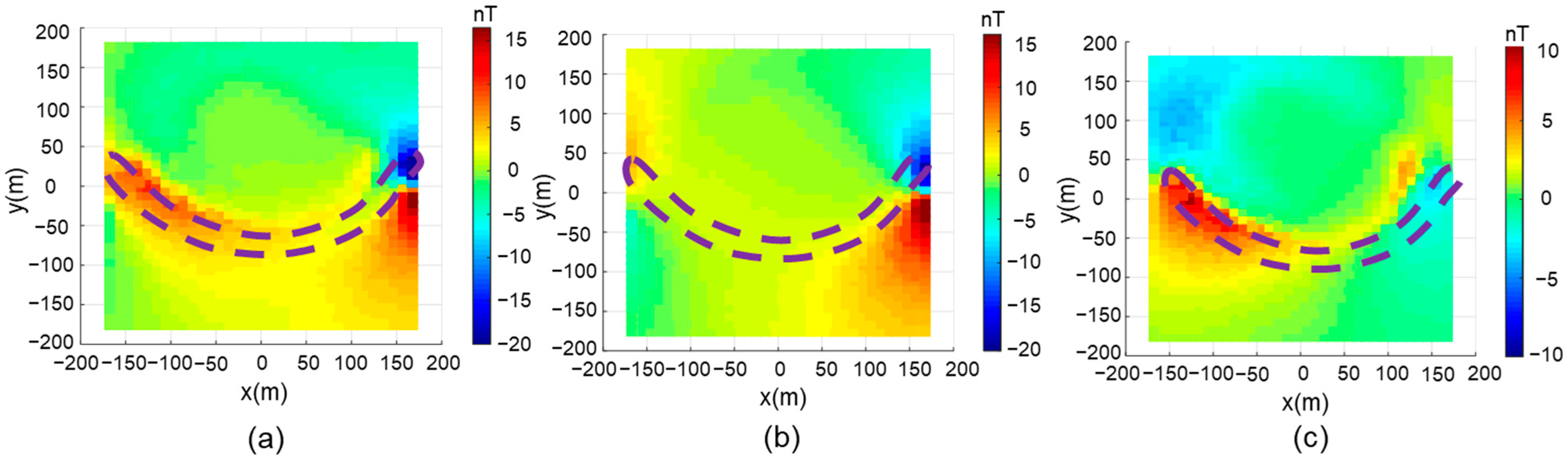
The anomalous SA-TFMMR data were simulated using the methodology outlined earlier. When the source orientation was optimally coupled to the fracture zone, a prominent positive anomaly coinciding with the fracture location was observed (Figure 3a,b). Subtracting the background response (without the fracture zone) from the coupled-field data (Figure 3c) accentuated the anomaly, revealing a peak amplitude of approximately 10 nT—a magnitude well within the detection range of modern high-precision magnetometers.

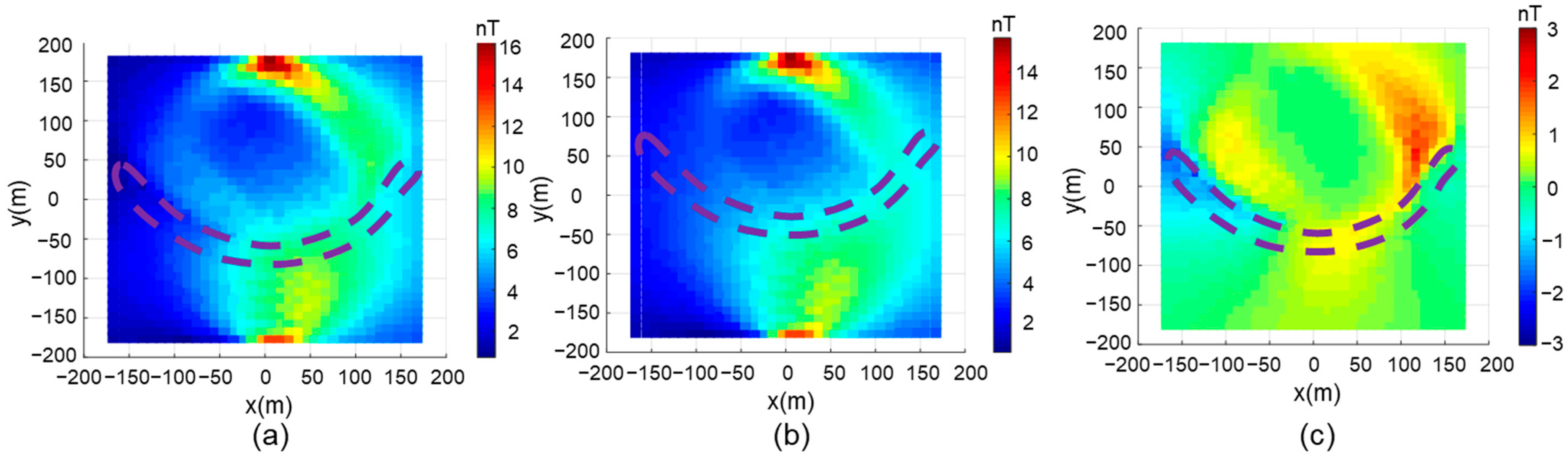
In contrast, when the source was oriented perpendicular to the fracture strike (null-coupled configuration), no discernible anomaly was observed due to minimal current channeling through the target (Figure 4a,b). The differential response (Figure 4c) exhibited a peak amplitude of only a few nT. This underscores the criticality of source placement in SA-TFMMR surveys, emphasizing the necessity of multi-orientation measurements to ensure robust target detection.

3.2. Influence of Target Body Orientation with Respect to Geomagnetic Field

The use of high-precision total-field magnetometers for TMI data acquisition effectively suppresses sensor motion-induced noise often seen in other airborne EM receivers because it measures the scalar magnitude of the geomagnetic field (|B|), eliminating the need for vector orientation corrections required by three-component magnetometers, which accumulate errors from sensor non-orthogonality (0.1–0.5° axis misalignment) and temporal mismatches between attitude sensors and magnetic data sampling. However, a potential issue arises when the direction of the magnetic field generated by MMR is orthogonal or nearly orthogonal to the direction of the geomagnetic field, resulting in TMI anomalous values close to zero.

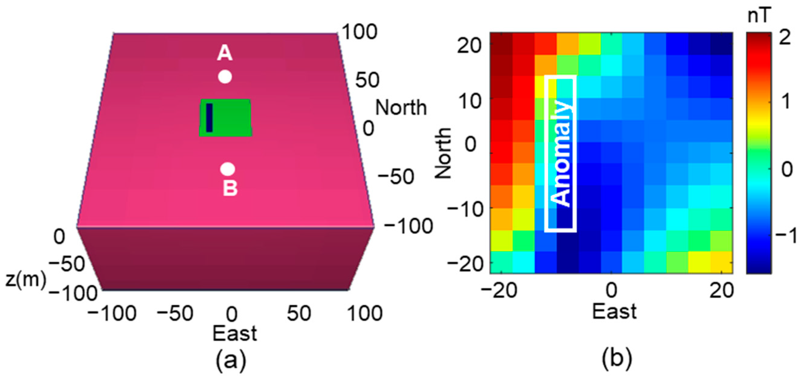
To illustrate the above, two synthetic models were designed in this study to simulate SA-TFMMR data. The background resistivity of the synthetic models is set to 1000 Ω·m, and the modeling domain is 200 m × 200 m × 100 m. The observation covers an area of 40 m × 40 m (green area in Figure 5), with the magnetometer suspended 2 m above the ground. The electrodes A and B are placed along the eastward coordinate axis in Model 1 (Figure 5a) and along the northward coordinate axis in Model 2 (Figure 6a), with an A-B electrode separation of 100 m and a burial depth of 1 m. A current intensity of 2 A is injected at the source electrodes. In both models, a conductive block with a resistivity of 100 Ω·m and a dimension of 30 m × 5 m × 4 m is buried at a depth of 2 m just 10 m off the central survey line in both models. The direction of the geomagnetic field is represented by a unit vector [−0.0439 0.8375 −0.5446], for which the x, y, and z-component represent the eastward, northward, and vertical directions, respectively.

When the direction of the underground current flow (object orientation) is west-east, there is a significant positive anomaly at the location of the anomaly body (white box in Figure 5b), with a peak value of approximately 8 nT. However, when the direction of the underground current flow is south-north, there is no prominent positive anomaly at the location of the anomaly body (white box in Figure 6b), and the peak value is only 2 nT. The data pattern in the south-north oriented survey lines and objects is also asymmetric and complicated by the local geomagnetic field direction. 3D inversion is required to decode the specific information about the object’s location, size, and orientation.

Therefore, it is necessary to consider the orientation of the sought geological objects relative to the geomagnetic field direction for MMR surveys using total field magnetometers. In reality, there are always current-channeling geological objects that are south-north oriented, so we propose a trade-off scheme to enhance the weakly coupled MMR signals in Figure 6b. In Figure 7, we test the deployment of the source electrodes in a northwest-southeast orientation, in which case a decent amount of current can still be channeled into the object, and the TMI anomaly due to the source excitation can be as parallel to the geomagnetic direction as possible.

3.3. Influence of Multi-Source Configurations

To evaluate the influence of multi-source configurations on subsurface imaging, this study compares inversion results from single-source and orthogonal-source deployments using an L-shaped blocky model. The results demonstrate that orthogonal source configurations significantly enhance imaging resolution for complex geological structures.

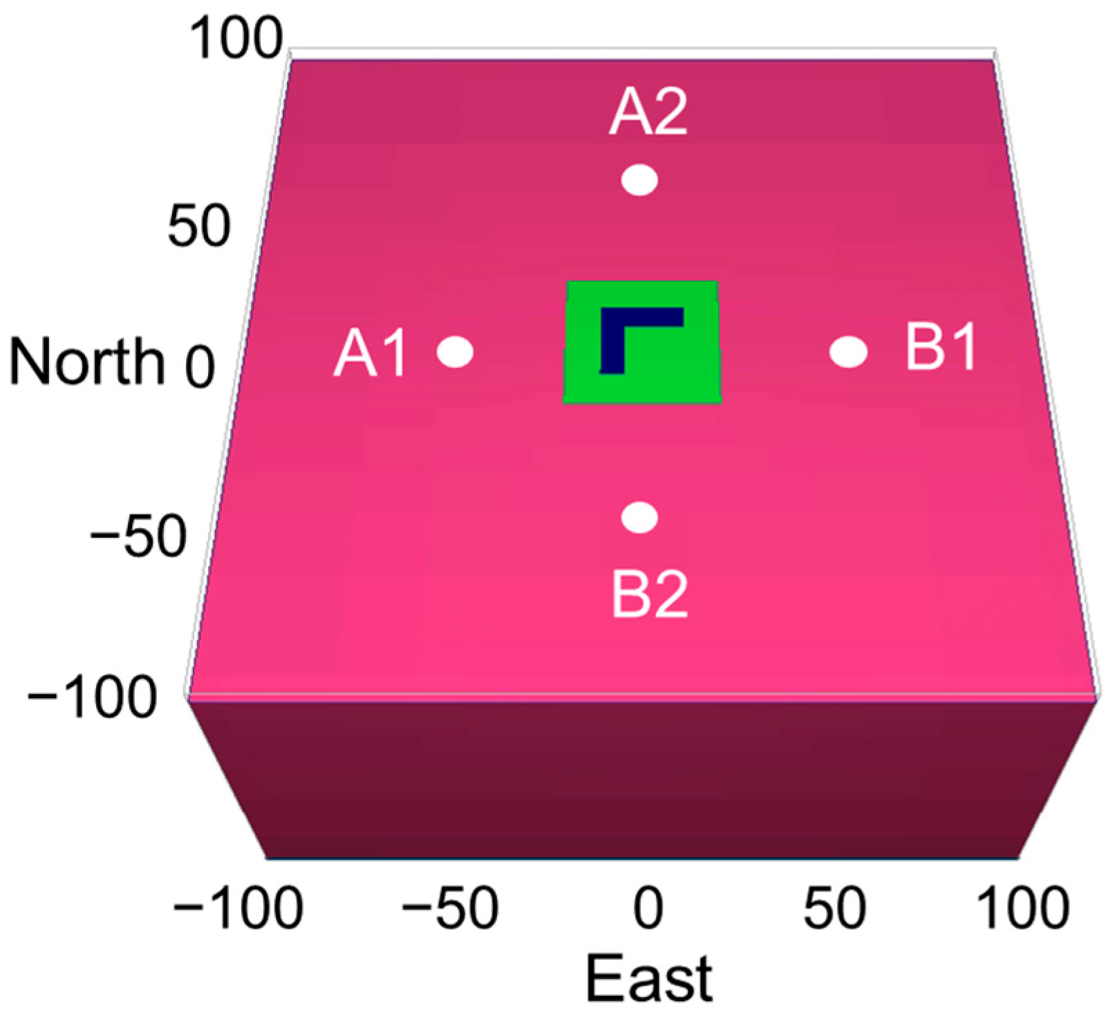
The L-shaped model (Figure 8) comprises two orthogonal rectangular prisms: one aligned east-west and the other north-south. Both prisms measure 20 m × 5 m × 4 m, are buried at a depth of 2 m, and have a resistivity of 100 Ω·m. The background resistivity, modeling domain, geomagnetic field parameters, and survey area (40 m × 40 m, green zone in Figure 8) remain consistent with those described in Section 3.1. Electrodes A1-B1 (east-west orientation) and A2-B2 (north-south orientation) are deployed with a separation of 100 m and a burial depth of 1 m, injecting a current of 2 A.

As demonstrated in Section 3.2, east-west-oriented current flow (electrodes A1-B1) generates a distinct positive anomaly at the location of the east-west-oriented target (Figure 9a). Inversion of these SA-TFMMR data achieves a misfit below 2% for over 90% of data points, indicating robust fitting accuracy (Figure 9c). However, cross-sectional slices of the inversion results (Figure 9d) reveal that the north-south prism remains unresolved. This limitation arises because the east-west current flow predominantly channels through the east-west prism, generating negligible magnetic anomalies from the north-south prism and thus insufficient constraints for its inversion.

To address this, orthogonal source electrodes A2-B2 (north-south orientation) were added to induce current flow through the north-south prism. Simultaneous inversion of datasets from A1-B1 and A2-B2 achieves a misfit below 3% for over 90% of data points (Figure 10c and Figure 11c), with cross-sectional slices (Figure 12) accurately reconstructing the L-shaped object’s locations, dimensions, and orientations. This confirms that mutually orthogonal source configurations provide complementary sensitivity to multi-directional subsurface structures, enabling a comprehensive imaging of complex anomalies.

Deploying orthogonal source pairs enhances the detectability of geometrically complex anomalies by leveraging directional current channeling. This approach mitigates the inherent limitations of single-source configurations, where the target orientation and geomagnetic field alignment dictate detection efficacy. The results underscore the necessity of multi-source deployment in SA-TFMMR surveys for robust subsurface characterization.

4. Inversion of a Dipping Water-Saturated Fracture Zone

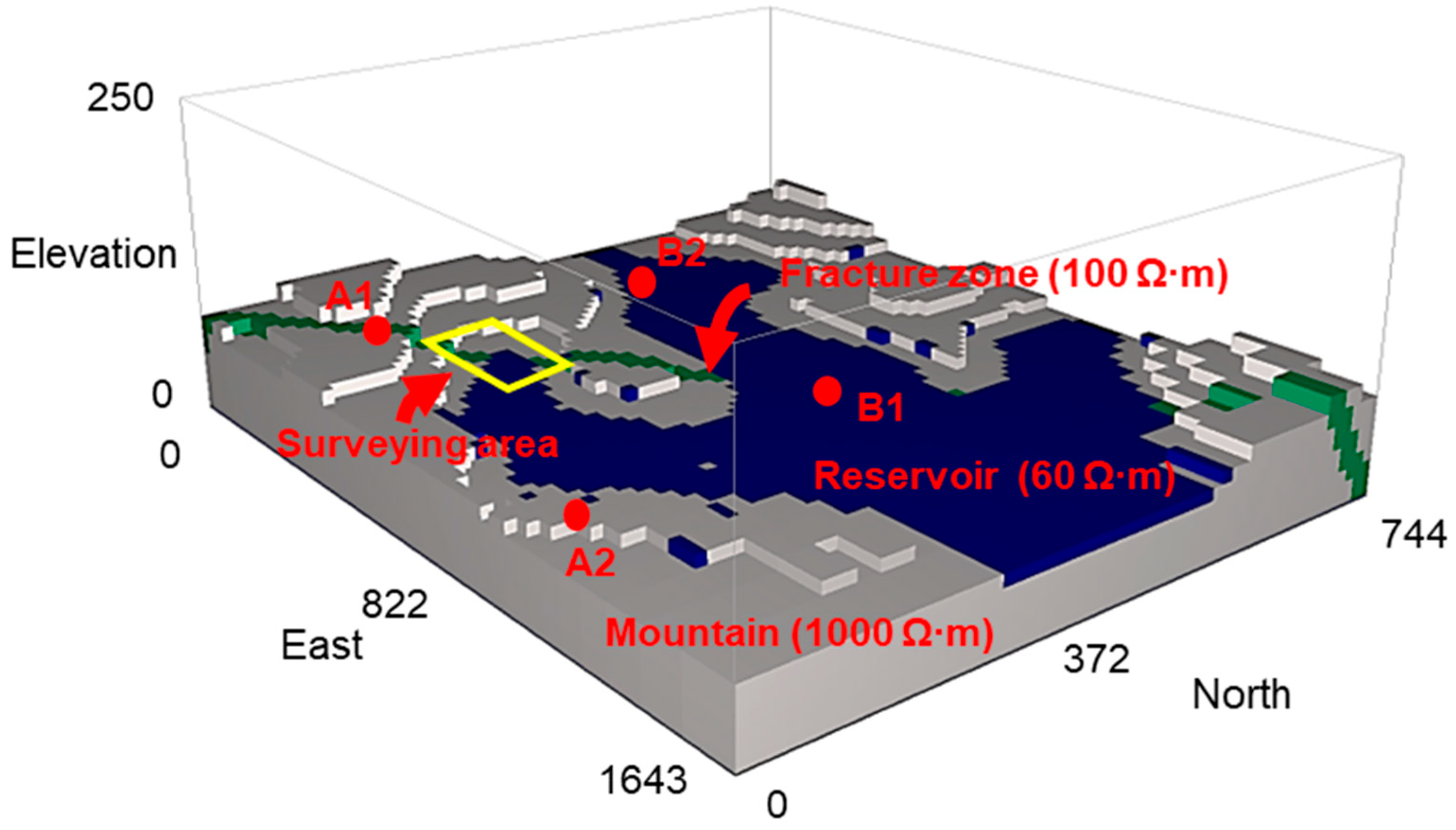
Building upon the sensitivity analysis and multi-source inversion strategies discussed in Section 3, this section validates the SA-TFMMR method’s capability to resolve geometrically complex, water-saturated fracture zones beneath conductive overburdens in mountainous terrains. The model integrates (1) a site-specific digital elevation model (DEM) and (2) geological maps from the 2021 water inrush accident at the Zhuhai Shijingshan Tunnel, with the incident location corresponding to the survey area highlighted by the yellow frame in Figure 13. On 15 July 2021, a catastrophic water-gushing accident occurred during the excavation of the Shijingshan Tunnel, where tunneling activities intersected a major regional fracture zone filled with weathered granites beneath the Jida Reservoir. Although pre-construction geological surveys had mapped the fracture zone, the sudden and catastrophic influx of groundwater through the fractures—which trapped and killed 14 workers—was entirely unanticipated. This disaster resulted from compounded factors, among which was the survey team’s failure to accurately assess the hydrogeological conditions of the fracture zone, particularly its high water-bearing capacity, thereby depriving construction planners of critical risk warnings.

This limitation originated from two factors: (1) topographic constraints preventing optimal sensor deployment and (2) low-resistivity water layers attenuating induced electromagnetic fields—a vulnerability addressed by SA-TFMMR’s terrain-adaptive 3D inversion framework. Our inversion reconstructs the fracture geometry through the integration of real-world DEMs and resistivity contrasts, demonstrating how terrain-aware geophysical modeling could have provided critical pre-construction risk warnings.

The synthetic mountain structure incorporates a northwest-dipping conductive fracture zone (Figure 13). The mountain and background medium (gray) exhibit a resistivity of 1000 Ω·m, while the reservoir (blue) and fracture zone (green) are assigned resistivities of 60 Ω·m and 100 Ω·m, respectively. The fracture zone, 20 m thick and dipping at 45° with a northwest-oriented normal vector, is embedded within the mountain and partially overlaid by a low-resistivity water layer. A high-precision magnetometer, suspended 5 m above the terrain surface by a UAV, acquired SA-TFMMR data over a 200 m × 200 m survey area (yellow frame in Figure 13), with a survey point spacing of 10 m (spatial resolution) and a total of 441 survey points, above the accident’s fracture zone, verifying the method’s pre-accident detection capability for the water-saturated fracture zone. The local geomagnetic field parameters include a background intensity of 45,332 nT, declination of −3°, and inclination of 33°. Two orthogonal electrode pairs—A1-B1 (parallel to the fracture strike, 581 m spacing) and A2-B2 (perpendicular to the fracture strike, 666 m spacing)—were deployed, each injecting a current of 2 A to probe directional sensitivity.

For 3D resistivity inversion, the subsurface model was discretized into 63 × 63 × 33 cells. The core region beneath the survey area utilized refined cells of 5 m × 5 m × 5 m, corresponding to half the survey point spacing (10 m), to ensure sufficient spatial resolution for reconstructing the fracture zone geometry. Synthetic data generated from forward modeling were contaminated with a 5% relative error to simulate realistic observational uncertainties. The initial model excluded the dipping fracture zone but preserved all other parameters of the synthetic structure (Figure 13). Computations were executed on an Intel i7-8700 CPU (3.2 GHz single-core frequency, 32 GB RAM), achieving convergence within nine iterations at approximately 1 min per iteration (total runtime: 10 min).

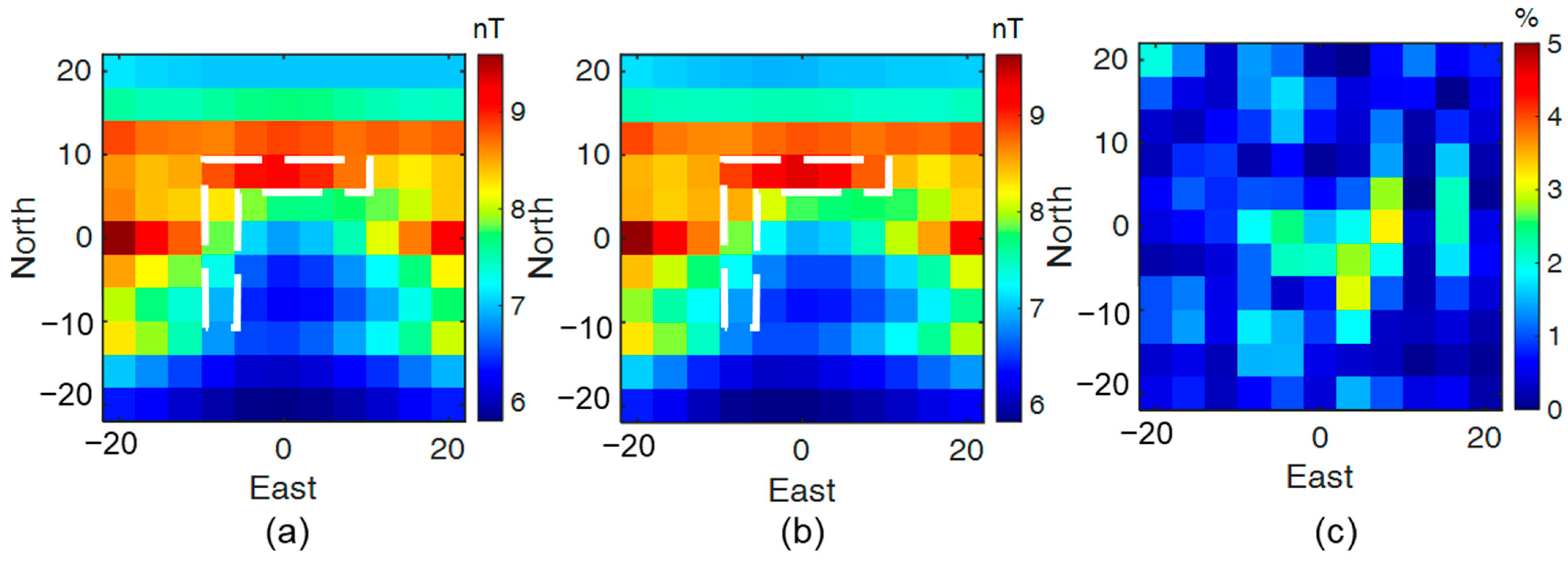
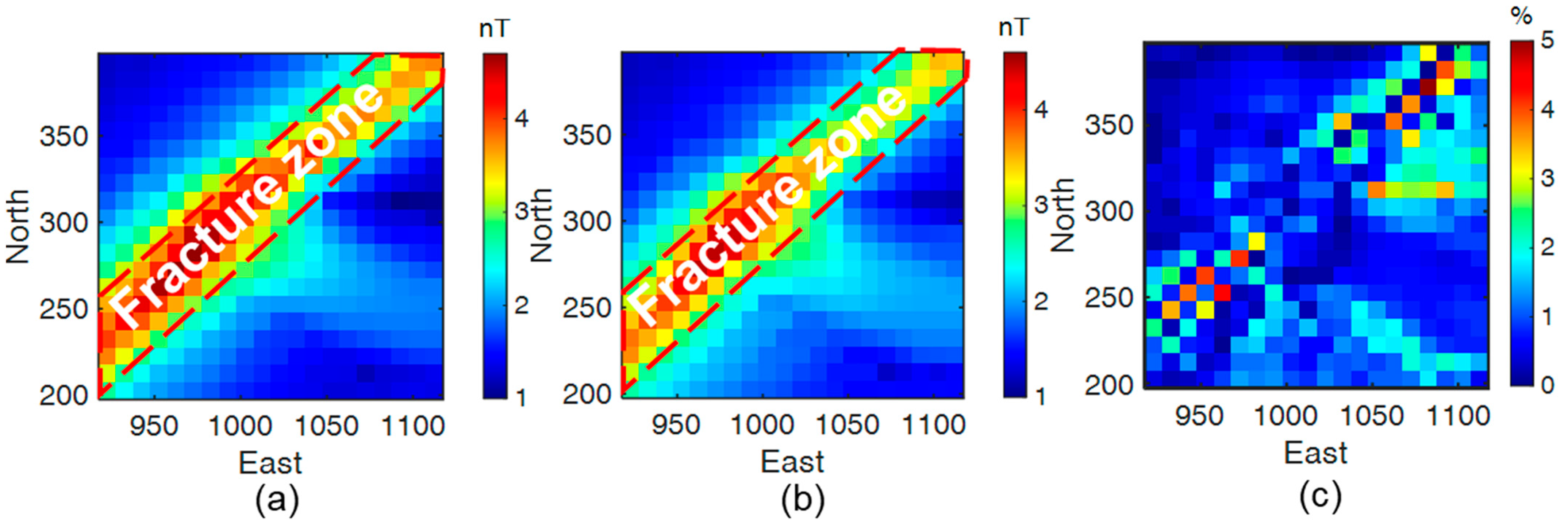
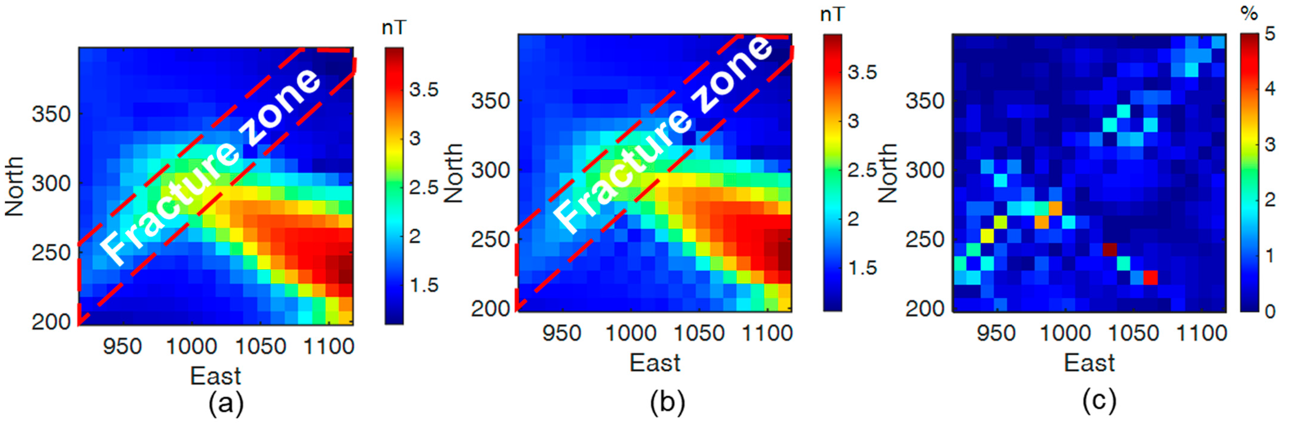
The SA-TFMMR data fitting results for both source configurations are presented in Figure 14 and Figure 15. The observed data (Figure 14a) exhibit distinct magnetic anomalies aligned with the fracture zone’s geometry, while the predicted data demonstrate strong consistency, with misfit values (Figure 14c and Figure 15c) below 5% for over 85% of data points. The orthogonal source configurations effectively capture the anisotropic current channeling effects caused by the fracture zone’s dipping structure, validating the multi-source strategy proposed in Section 3.

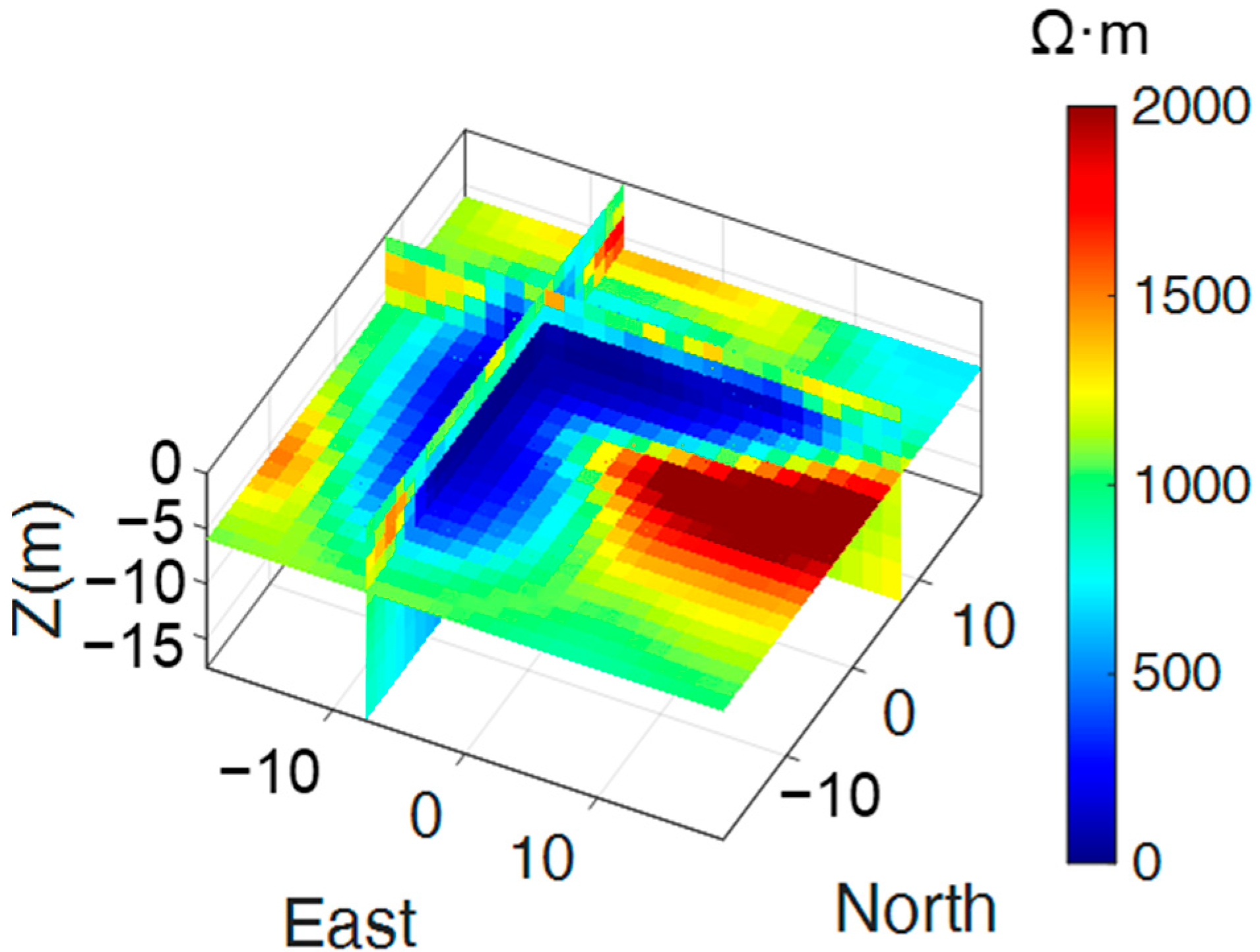
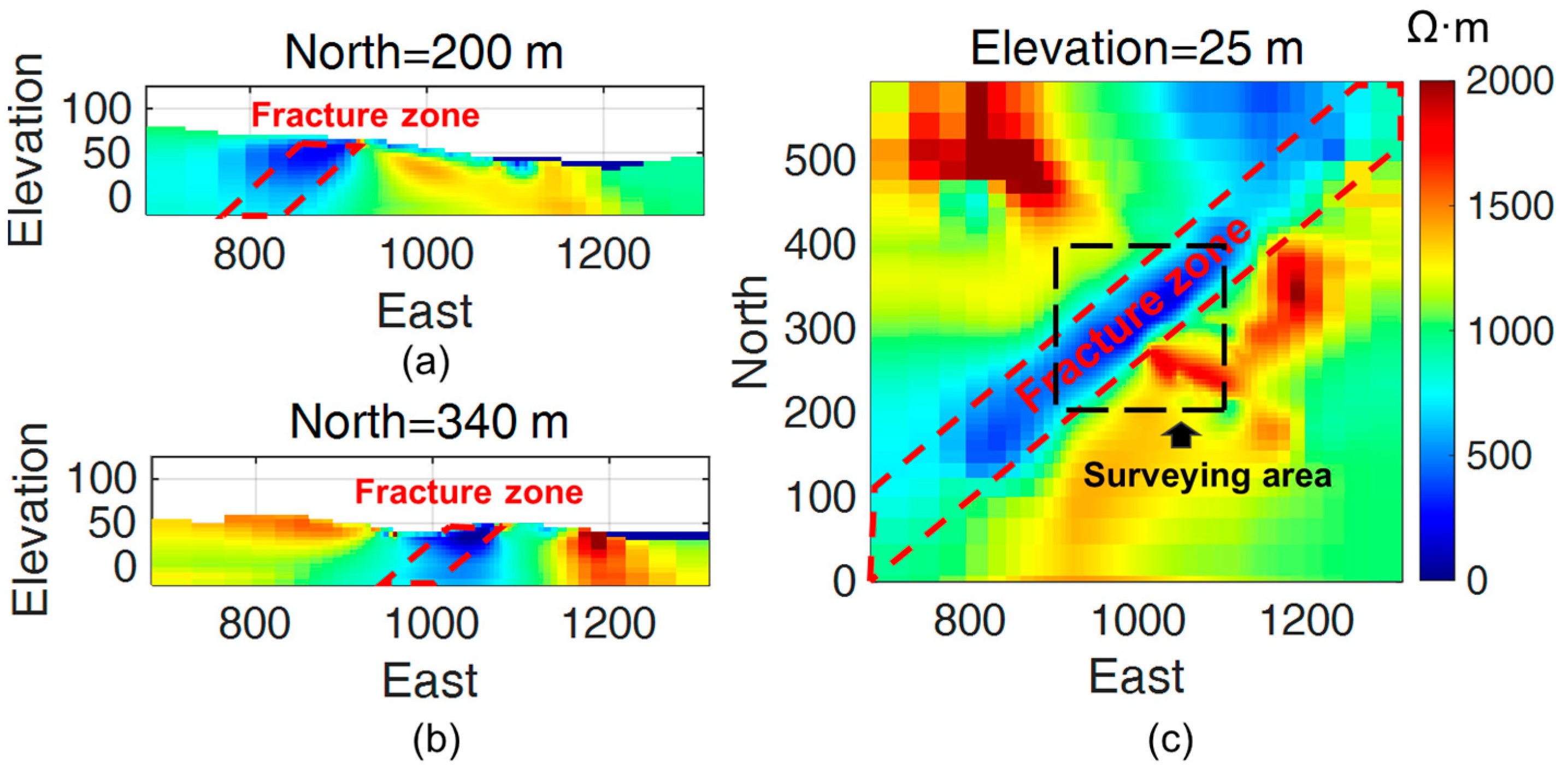
The three-dimensional inversion results are illustrated in Figure 16. Vertical slices at northings 200 m (Figure 16a) and 340 m (Figure 16b) reveal the dipping geometry of the low-resistivity target (red dashed lines), with a reconstructed dip angle of approximately 45°, consistent with the model setup. The slice at 25 m elevation (Figure 16c) further confirms the fracture zone’s lateral position and resistivity (~100 Ω·m), consistent with the synthetic parameters. These results highlight the method’s ability to resolve both the spatial extent and orientation of dipping fracture zones, even when partially obscured by the overlying water layers.

The successful 3D inversion of this realistic model underscores the SA-TFMMR method’s adaptability to complex terrains and heterogeneous subsurface structures. By combining the orthogonal source configurations with the optimal source-target coupling, the method mitigates ambiguities arising from the nonlinear relationship between the target geometry and magnetic responses. The dipping fracture zone’s accurate reconstruction—despite its partial overlap with a conductive overburden—demonstrates the method’s robustness against shielding effects, a critical advantage in hydrogeological and engineering applications.

The SA-TFMMR method’s ability to resolve dipping fracture zones, even under challenging topographic and geological conditions, positions it as a promising tool for infrastructure planning, landslide risk assessment, and groundwater exploration in mountainous regions. Future work will focus on field validations and the integration of additional geophysical datasets to further refine inversion accuracy

5. Discussion

While promising results were obtained through synthetic data analysis in previous sections, the practical implementation of the SA-TFMMR method necessitates addressing additional challenges in field surveys, such as UAV-induced noise contamination and dead-zone effects inherent to total-field magnetometers. To evaluate the method’s operational limits and detection capabilities, this section analyzes an SA-TFMMR field dataset acquired using the same UAV-borne system under real-world conditions.

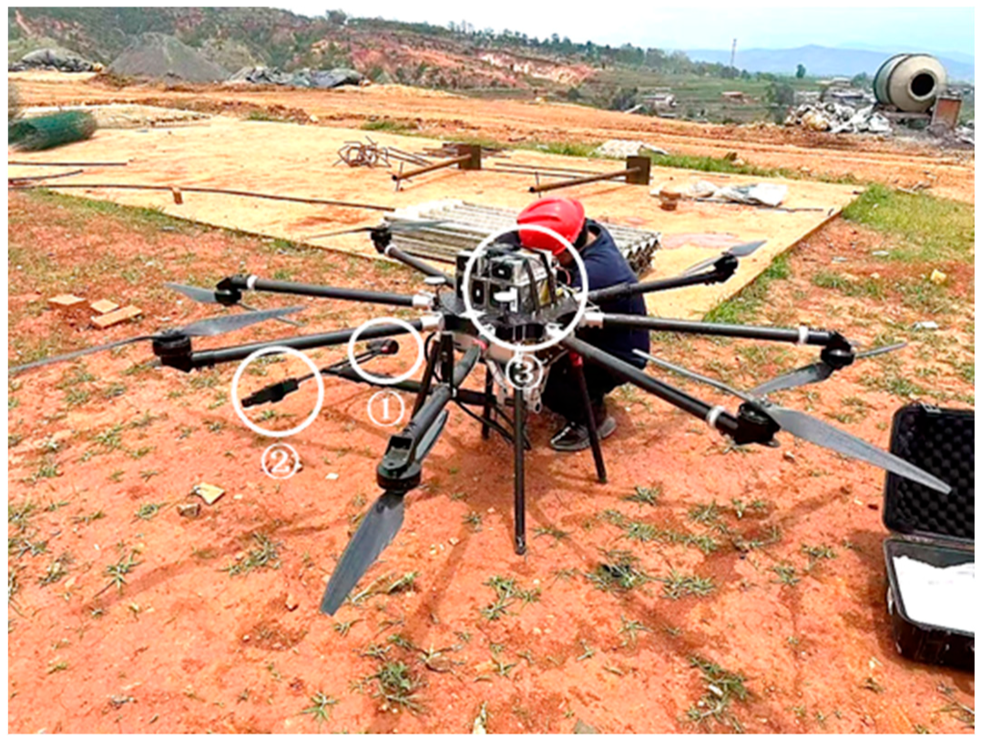
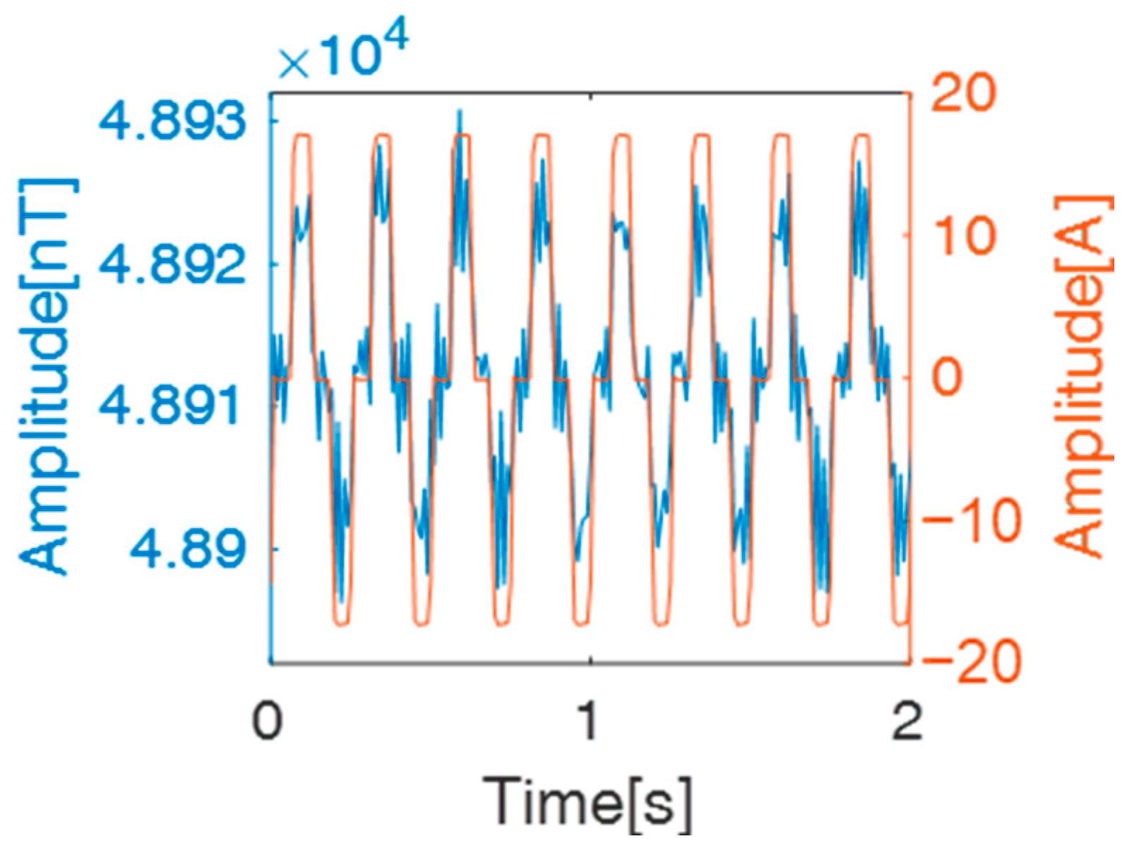
In our field experiment, a high-power transmitter injected bipolar square-wave signals at 4 Hz with a peak current of 17.4 A through grounded electrodes (AB configuration), generating an artificially induced electromagnetic field. The receiver system comprised a DJI M600 Pro UAV equipped with a high-precision cesium optical-pumping magnetometer (hereafter referred to as the cesium magnetometer system). The UAV operated at an average flight altitude of 117 m above the mean sea level and a speed of 5 m/s. As illustrated in Figure 17, the cesium magnetometer system (Beijing Orangelamp Geophysical Exploration Co., Ltd. China) integrates multiple critical components: ① a cesium optical-pumping probe, ② a fluxgate sensor, and ③ auxiliary modules including a data logger, attitude compensation unit, high-precision positioning system (RTK/GPS), inertial measurement unit (IMU; roll/pitch/yaw accuracy <1°), altimeter, and power management system. A LiDAR system (2.2 kg) was additionally deployed for pre- or post-experiment terrain mapping. With a detection range of 260 m and ranging accuracy of ±2 cm, the LiDAR conducted separate flights to obtain high-resolution digital elevation models (DEMs) of the survey area.

The DJI M600 Pro UAV features a hexacopter airframe constructed from high-strength carbon fiber composites, achieving an optimal balance between structural rigidity and lightweight design. With a maximum takeoff weight of 15.5 kg, payload capacity of 6 kg, and endurance of 42 min, it demonstrates superior logistical adaptability for field operations. The cesium optical-pumping probe, serving as the core sensor, exhibits a dynamic noise floor below 0.01 nT, with repeatability errors of <1 nT along survey lines and <0.8 nT at crossover points—performance metrics fully compliant with SA-TFMMR detection requirements. The data acquisition system operated at a sampling rate of 100 Hz to ensure the full-bandwidth capture of SA-TFMMR signals, achieving a system white noise level of 0.3 pT and a resolution of 0.0001 nT for the reliable detection of weak signals.

The fluxgate probe (±100 μT full-scale range, internal noise ≤6–8 pT rms/√Hz) monitored real-time UAV-induced magnetic interference, while the IMU and RTK module (horizontal positioning error: ±2 cm; vertical error: ±3 cm) provided foundational support for the spatial registration and dynamic compensation of magnetic data. Magnetic compensation flights were conducted in an anomaly-free flat area adjacent to the survey zone to ensure environmental field homogeneity.

Robust data processing methodologies form the cornerstone of translating theoretical models into engineering applications. Failure to accurately extract theoretically consistent responses from raw observational data will inevitably lead to distorted inputs for inversion processes, thereby compromising the reconstruction of reliable subsurface resistivity structures. Then, we analyzed a representative survey line from our field experiment. Given the transmitter’s bipolar current frequency of 4 Hz and the UAV’s flight speed of 5 m/s, the survey point interval was set to 10 m, corresponding to a 2-s time series per survey point (Figure 18), encompassing eight complete waveforms (16 independent measurement windows of alternating polarity).

The total magnetic intensity (TMI) measured by the magnetometer comprises three parts: the background geomagnetic field (B₀), rock magnetization anomalies (Ba), and the SA-TFMMR response from target bodies due to the artificial excitation (B_SA-TFMMR). The core methodology for isolating the target SA-TFMMR signal lies in bipolar differential processing. The workflow is detailed as follows:

When a bipolar current (red line in Figure 18) is injected through electrodes A-B, the observed TMI anomaly during the positive half-cycle can be expressed as:

$$\left|{\mathbf{B}}_0+{\mathbf{B}}_{\mathrm{a}}+{\mathbf{B}}_{\mathrm{M}\mathrm{M}\mathrm{R}}\right|-\left|{\mathbf{B}}_0\right|\approx \left({\mathbf{B}}_{\mathrm{a}}+{\mathbf{B}}_{\mathrm{M}\mathrm{M}\mathrm{R}}\right)·\widehat{{\mathbf{B}}_0}={\mathbf{B}}_{\mathbf{a}}·\widehat{{\mathbf{B}}_0}+{\mathbf{B}}_{\mathrm{M}\mathrm{M}\mathrm{R}}·\widehat{{\mathbf{B}}_0}$$

(12)

where $\widehat{{\mathit{B}}_0}$ denotes the unit vector of the geomagnetic field. Conversely, during the negative half-cycle:

$$\left|{\mathbf{B}}_0+{\mathbf{B}}_{\mathrm{a}}-{\mathbf{B}}_{\mathrm{M}\mathrm{M}\mathrm{R}}\right|-\left|{\mathbf{B}}_0\right|\approx \left({\mathbf{B}}_{\mathrm{a}}-{\mathbf{B}}_{\mathrm{M}\mathrm{M}\mathrm{R}}\right)·\widehat{{\mathbf{B}}_0}={\mathbf{B}}_{\mathbf{a}}·\widehat{{\mathbf{B}}_0}-{\mathbf{B}}_{\mathrm{M}\mathrm{M}\mathrm{R}}·\widehat{{\mathbf{B}}_0}$$

(13)

Theoretically, combining Equations (12) and (13) enables the cancellation of both B₀ and Ba, yielding the isolated SA-TFMMR response:

$${\mathrm{B}}_{\mathrm{S}\mathrm{A}-\mathrm{T}\mathrm{F}\mathrm{M}\mathrm{M}\mathrm{R}}={\mathbf{B}}_{\mathrm{M}\mathrm{M}\mathrm{R}}·\widehat{{\mathbf{B}}_0}={\displaystyle \frac{1}{2}}(\left|{\mathbf{B}}_0+{\mathbf{B}}_{\mathrm{a}}+{\mathbf{B}}_{\mathrm{M}\mathrm{M}\mathrm{R}}\right|-\left|{\mathbf{B}}_0+{\mathbf{B}}_{\mathrm{a}}-{\mathbf{B}}_{\mathrm{M}\mathrm{M}\mathrm{R}}\right|)$$

(14)

This operation suppresses interference from geomagnetic diurnal variations and low-frequency noise (<4 Hz).

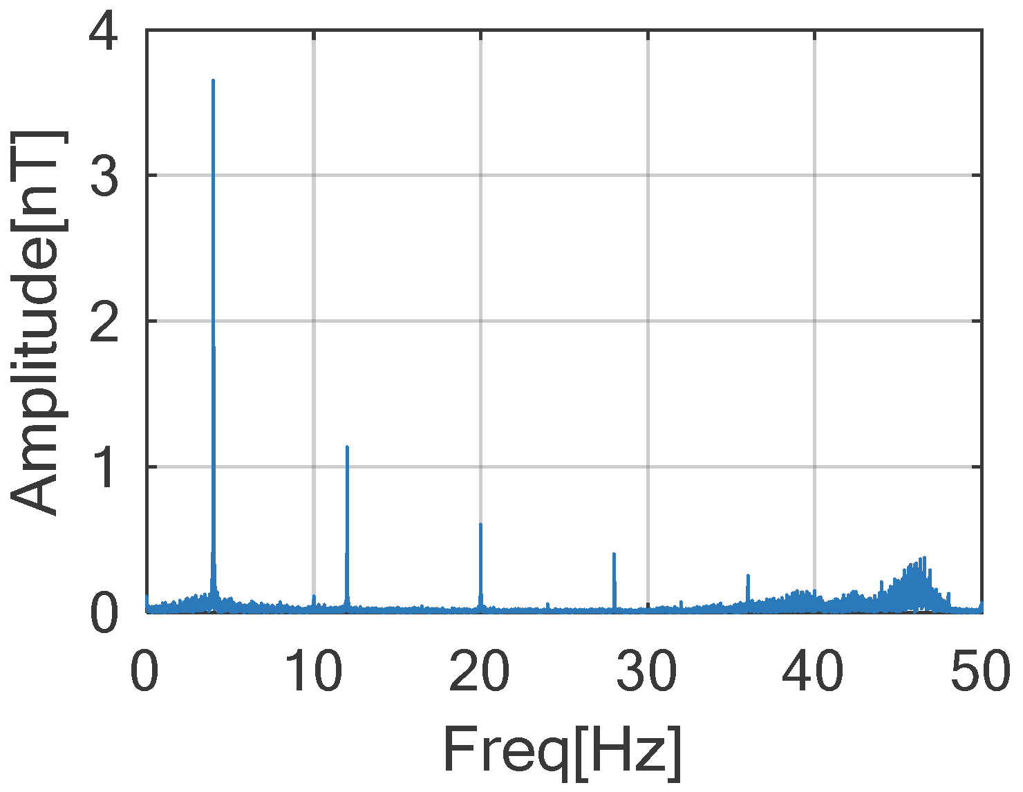
To evaluate the impact of high-frequency noise (e.g., UAV-induced interference), we performed a Fast Fourier Transform (FFT) analysis on the preprocessed magnetic signals after removing diurnal variations and low-frequency noise. The single-sided amplitude spectrum (Figure 19) reveals dominant noise components in the 35–48 Hz range, exceeding the 16 Hz threshold.

To mitigate these effects, data from each independent measurement window (positive or negative half-cycle window, 1/16 s duration) were stacked. Specifically, the stacked negative half-cycle data were phase-reversed and averaged with the stacked positive half-cycle data across all 16 windows, significantly enhancing signal fidelity.

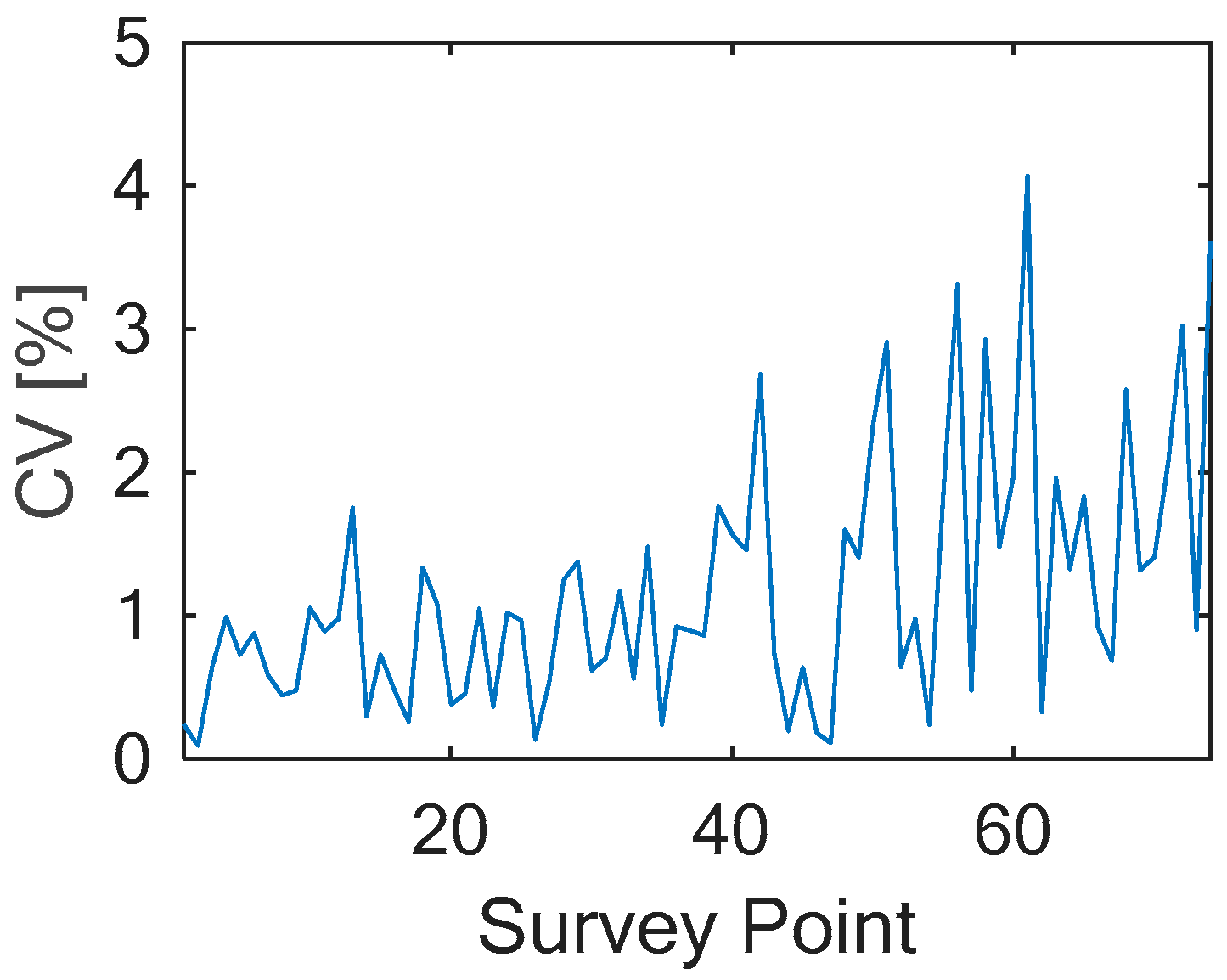
As previously described, 16 independent measurement windows were utilized to acquire SA-TFMMR responses at each survey point. To quantify data variability, the coefficient of variation (CV) was adopted as a statistical metric for assessing fluctuations. For each survey point’s 16-window averaged dataset, the CV is defined as:

$$\mathrm{C}\mathrm{V}={\displaystyle \frac{\sigma }{\mu }}\times 100\%$$

(15)

where σ and μ represent the standard deviation and arithmetic mean of the window-averaged values, respectively. This normalized metric effectively captures relative data variability, with CV < 5% indicating spatially consistent responses. The CV profile across all survey points along the test line is shown in Figure 20.

Our results revealed that all survey points exhibit CV values below 5%, achieving dual objectives: (1) validating the efficacy of the proposed data extraction methodology and (2) confirming that the 5% relative error assigned to observed data during inversion appropriately accounts for operational variability in field conditions.

To explore the detection capability of the SA-TFMMR method and validate the efficacy of its signal extraction workflow, we systematically analyzed synthetic datasets with varying signal-to-noise ratios (SNRs). The normalized mean squared error (NMSE) was adopted as a quantitative metric to evaluate deviations between extracted and ground-truth SA-TFMMR responses. Synthetic tests spanning SNRs of 1–30 dB (Figure 21) revealed distinct performance tiers.

In high SNR regimes (≥14 dB), NMSE values consistently remained below 0.01, indicating minimal deviation between extracted and true responses. For moderate SNR ranges (4–14 dB), NMSE values generally stayed below 0.1, suggesting minor waveform distortion that still preserved sufficient fidelity for inversion requirements. Under low SNR conditions (<4 dB), however, NMSE escalated sharply, accompanied by severe waveform distortion, marking the method’s operational limit under poor signal conditions.

This study delineates the practical constraints of SA-TFMMR, including equipment parameters, UAV-induced noise, and SNR-dependent detection thresholds. Critical limitations identified include (1) dead-zone effects: rigid mounting of the cesium magnetometer on the UAV airframe risk misalignment with the geomagnetic field vector, compromising measurement accuracy; and (2) persistent UAV noise: weak SA-TFMMR signals (<4 dB SNR) become indistinguishable from ambient noise. While increasing transmitter current can enhance signal strength, this approach escalates logistical complexity and power consumption.

To address these challenges, we propose the following advancements for future iterations: (1) Multi-axis magnetometer arrays: Deploying orthogonally oriented magnetometers to ensure continuous valid measurements regardless of UAV attitude. (2) Tethered sensor deployment: adopting a suspended magnetometer configuration—where the sensor is tethered beneath the UAV via non-magnetic cabling—could isolate the instrument from UAV-induced noise, thereby enhancing signal-to-noise ratios (SNRs) without escalating transmitter power requirements. (3) High-sampling-rate magnetometers: integrating next-generation magnetometers with higher sampling rates (>200 Hz) and sub-picotesla sensitivity would improve the resolution of transient anomalies while enabling real-time adaptive filtering of high-frequency noise. These synergistic enhancements aim to overcome current operational constraints, extending SA-TFMMR’s applicability to electromagnetically complex and topographically extreme environments.

6. Conclusions

The drone-based semi-airborne total-field magnetometric resistivity (SA-TFMMR) method establishes a novel paradigm for geophysical exploration in geologically complex terrains where conventional surface-based methods face insurmountable limitations. By integrating drone-deployed total-field magnetometers with ground-based current injection, this approach eliminates motion artifacts inherent to induction coil systems while mitigating electromagnetic interference in urbanized environments. The development of a terrain-adaptive 3D inversion framework incorporating digital elevation models (DEMs) enables the high-fidelity reconstruction of geometrically intricate subsurface structures, overcoming the challenge of imaging water-saturated fracture zones in mountainous regions.

Key findings from sensitivity analyses reveal that the source-target coupling and geomagnetic field orientation significantly govern SA-TFMMR’s detection efficacy. Optimal alignment of current injection directions with target geometries amplifies magnetic anomalies, whereas a null-coupled source orientation suppresses the anomalous data. The multi-source inversion strategy, validated through synthetic and realistic models, enhances imaging accuracy for geometrically complex structures, such as dipping fracture zones, by leveraging complementary datasets.

The application of SA-TFMMR to a synthetic mountainous model with a 45-dipping fracture zone underscores its practical utility. Inversion results successfully reconstructed the fracture zone’s spatial extent, resistivity contrast (~100 Ω·m), and dip angle. These outcomes highlight the method’s robustness in recovering low-resistivity features under conductive overburdens, a critical capability for infrastructure risk assessment, geohazard mitigation, and hydrogeological and engineering applications. For practical implementation, SA-TFMMR holds promise for infrastructure planning, landslide risk assessment, and groundwater exploration in mountainous regions.

This work advances UAV geophysics through three key innovations:

• Total-field magnetometer deployment. Replacing induction coils with high-precision total-field magnetometers to eliminate motion-induced noise, enabling reliable UAV-borne magnetic measurements even in dynamic flight conditions.
• Low-frequency galvanic excitation. Utilizing grounded current injection at 4 Hz to overcome electromagnetic shielding from conductive overburdens, uniquely enhancing sensitivity to deep fracture zones.
• Multi-source inversion with DEM constraints. Integrating orthogonal source datasets and UAV-derived topography into a unified 3D inversion framework, enabling geometrically accurate imaging of dipping structures—a breakthrough beyond traditional MMR methods limited to flat terrains.