Prescribed Performance Sliding Mode Fault-Tolerant Tracking Control for Unmanned Morphing Flight Vehicles with Actuator Faults

Abstract

This article focuses on the prescribed performance sliding mode fault-tolerant control problem for an unmanned morphing flight vehicle (MFV) with actuator faults and composite disturbances during wing deformation. Firstly, the longitudinal nonlinear dynamic model of the unmanned MFV is introduced. Then, a control framework is proposed by decomposing the integrated dynamic model into attitude and velocity subsystems, effectively simplifying controller architecture and improving fault tolerance. Further, the constrained tracking errors are systematically transformed into unconstrained counterparts via projection operators to facilitate controller design. For each subsystem, a prescribed performance sliding mode fault-tolerant controller is developed, ensuring both transient performance and steady-state tracking accuracy. Finally, the simulation results verify the feasibility and effectiveness of the proposed fault-tolerant control strategy.

1. Introduction

Unmanned morphing flight vehicles (MFVs) achieve unprecedented mission adaptability through structural reconfiguration, enabling expanded flight envelopes and enhanced maneuverability [1,2,3]. Their inherent challenges stem from high-dimensional nonlinear coupled dynamics, actuator degradation vulnerability under morphing-induced transients, and measurement reliability deterioration during configuration transitions. These compounded effects critically undermine operational safety while revealing existing control frameworks’ deficiencies in addressing parametric uncertainties and guaranteeing transient performance. The development of rigorous fault-tolerant control (FTC) architectures thus constitutes a pivotal challenge in aerospace control theory.

A variety of advanced control methodologies have been effectively developed and applied in the field of unmanned MFV. These methods can generally be categorized into two major approaches: linear control and nonlinear control. Linear control methodologies include classical proportional integral derivative (PID) control [4], linear quadratic regulator (LQR) control [5], gain-scheduling control [6,7], and linear parameter-varying (LPV) control [8,9]. These methods (except LPV) predominantly rely on linearized equilibrium point models and struggle to accommodate significant state deviations caused by the wide flight envelope of unmanned MFVs. Although the LPV method improves applicability via time-varying parameter modeling, it overlooks morphological dynamics’ nonlinearity [10], while robustness-induced conservatism restricts controller dynamics, ultimately failing to satisfy flight control’s stringent responsiveness demands. Considering the intrinsic nonlinearity and coupling characteristics of unmanned MFV, nonlinear control methodologies such as backstepping control [11,12,13], nonlinear dynamic inversion (NDI) [14], and adaptive control [15,16] enable controllers to tolerate or even compensate for unmodeled system components and external disturbances during flight, thereby ensuring steady-state tracking performance. However, these methods still heavily depend on model accuracy. Notably, sliding mode control (SMC) [17,18,19] has gained significant popularity in unmanned MFV control due to its strong robustness against model uncertainties and external disturbances. Nevertheless, conventional SMC inherently exhibits chattering phenomena while showing actuator-saturation risks under compound faults, necessitating prescribed transient regulation to enforce dynamic constraints.

A critical deficiency in unmanned MFV control system design stems from the persistent oversight of transient dynamics management within existing control techniques. This oversight substantially undermines overall control efficacy, particularly given the stringent dynamic performance demands imposed by unmanned MFV configurations. In this article, prescribed performance control (PPC) has gained widespread attention in aerospace applications. The principal strength of this approach resides in its ability to quantitatively characterize both the transient and steady-state performance of controlled systems under system constraints [20]. It exhibits strong robustness against diverse faults and uncertainties, and allows for flexible control-law design tailored to specific performance requirements and system characteristics. Currently, PPC has been successfully implemented in fields such as robotic manipulators [21,22], unmanned aerial vehicles [23,24], and hypersonic vehicles [25,26,27]. Current investigations into PPC-based fault-tolerant tracking controllers for disturbance-affected unmanned MFV systems under simultaneous actuator failures remain fundamentally underdeveloped. This work addresses this gap.

Another critical challenge in unmanned MFV development involves ensuring a reliable FTC scheme during actuator fault conditions. Current FTC paradigms predominantly adopt either active or passive methodologies. Although active FTC exhibits lower conservatism, it faces challenges such as abrupt controller reconfiguration and time delays in fault detection and isolation, which reduce the reliability of control systems in actual flight operations. Therefore, passive FTC proves more suitable for handling sudden actuator failures in morphing flight vehicles. This approach achieves prescribed robustness guarantees without requiring online fault estimation or control law reconfiguration—a decisive advantage for safety-critical aerospace systems [28].

Recent advances in passive FTC methodologies for unmanned MFVs demonstrate various technical pathways. Wen et al. [29] proposed a model reconstruction architecture employing infinite-time robust adaptive linear quadratic (LQ) compensation to capture actuator-induced phase mutations through time-varying system identification. Yuan [10] and Chao [30] developed passive FTC strategies based on adaptive backstepping, effectively mitigating actuator failure impacts using the universal approximation capability of a radial-basis-function neural network (RBFNN). Liu [31] and Liang [32] incorporated disturbance observer techniques into passive FTC design, achieving faster fault adaptation and improving tracking precision. Liu et al. [33] designed parameter update laws and adaptive controllers with a control allocation algorithm, combining fixed and adaptive allocation ratios to address vehicle uncertainties, compensate actuator failures, and suppress actuator saturation for desired tracking performance. Considering reliability and safety, it is crucial to ensure the stability of the transient performance under actuator-induced adverse effects. However, existing FTC methods neglect transient performance considerations, which would significantly compromise control effectiveness for unmanned MFVs experiencing system failures. Moreover, the high computational loads of current FTC schemes may limit their practical implementation in unmanned MFVs. Therefore, developing a prescribed performance FTC strategy with lower computational burden holds significant practical importance for unmanned MFV applications.

Based on the aforementioned research background, this article proposes a prescribed performance sliding mode fault-tolerant controller for unmanned MFVs. As illustrated in the proposed control framework (Figure 1), the methodology sequentially applies PPC to convert constrained errors into unconstrained ones, decouples the unmanned MFV system model into attitude and velocity subsystems, and designs dedicated prescribed performance sliding mode fault-tolerant controllers (“SMC+PPC”) for each subsystem. The figure further clarifies signal-propagation paths and fault-compensation mechanisms across modules. The core innovations of this study are reflected in three aspects:

(1)

By decomposing the integrated dynamics into attitude and velocity subsystems, the developed framework simplifies controller architecture and improves fault tolerance characteristics. This decomposition effectively mitigates control complexity arising from high-dimensional coupling effects;

(2)

Unlike existing approaches [10,11,12,14,15,17,29,30,31,32,33,34,35,36] that only ensure steady-state performance, the proposed “SMC+PPC” guarantees both transient performance and tracking-error compliance with prescribed performance constraints;

(3)

Compared to methods in the Refs. [10,30,31,32], the proposed modular scheme demonstrates a lower computational burden. By integrating SMC with PPC, the scheme achieves rapid response to reduce conservatism and enhances fault tolerance through switching control laws, thereby improving stability. These synergistic merits enhance its practical value in engineering applications.

The paper proceeds as follows: Section 2 formulates the unmanned MFV dynamical model with actuator faults and composite disturbances. Section 3 develops the “SMC+PPC” fault-tolerant control architecture. Section 4 provides a numerical validation of the FTC scheme’s efficacy, culminating in concluding remarks in Section 5.

2. Problem Formulation

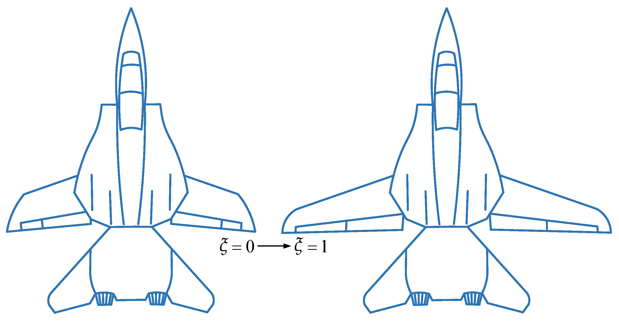
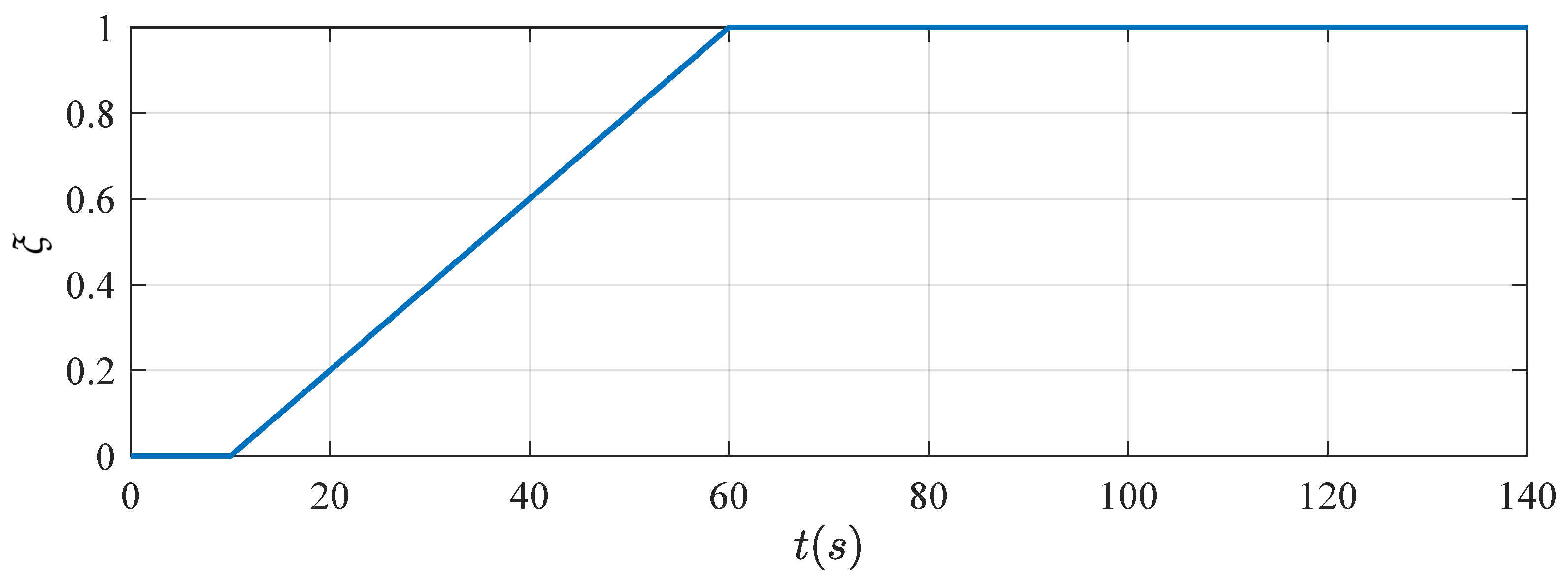
2.1. The Longitudinal Nonlinear Dynamics Model of the Unmanned MFV

This study focuses on a variable wingspan aircraft as the research subject, which is capable of autonomously adjusting its wingspan length during flight. The wings on both sides symmetrically extend or retract (as illustrated in Figure 2). The wingspan deformation rate $\xi$ ranges from 0 to 1.

The longitudinal nonlinear dynamics of the unmanned MFV are modeled as [37,38]

$$\dot{x}=\left\{\begin{array}{c}\dot{V}={\displaystyle \frac{Tcos\alpha }{m}}-{\displaystyle \frac{D\left(\xi \right)}{m}}-gsin(\theta -\alpha )\hfill \\ \dot{\alpha }=q-{\displaystyle \frac{Tsin\alpha }{mV}}-{\displaystyle \frac{L\left(\xi \right)}{mV}}-{\displaystyle \frac{gcos(\theta -\alpha )}{V}}\hfill \\ \dot{\theta }=q\hfill \\ \dot{q}={\displaystyle \frac{M_y\left(\xi \right)}{I_y}}\hfill \\ \dot{h}=Vsin(\theta -\alpha )\hfill \end{array}\right.$$

(1)

where m denotes the vehicle mass. V and h are the unmanned MFV velocity and altitude, respectively. g represents the gravitational acceleration. $L\left(\xi \right),D\left(\xi \right),T$ are the lift, drag, and thrust, respectively. $\alpha ,\theta ,q$ represent the angle of attack, the pitch angle, and the pitch rate, respectively. $I_y$ and $M_y\left(\xi \right)$, respectively, denote the pitch moment of inertia and the pitching moment about the unmanned MFV body y-axis. Specifically, the longitudinal aerodynamic and aerodynamic torque $L\left(\xi \right),D\left(\xi \right),M_y\left(\xi \right)$ are functions of $\xi$, expressed as

$$\left\{\begin{array}{c}L=Q{S}_w{C}_L\left(\xi \right)\hfill \\ D=Q{S}_w{C}_D\left(\xi \right)\hfill \\ M_y=Q{S}_w{c}_A{C}_m\left(\xi \right)\hfill \end{array}\right.$$

(2)

where $Q=0.5\rho V^2$ denotes the dynamic pressure, $\rho$ is the atmospheric density, $S_w$ and $c_A$ are the wing reference area and mean geometric chord of the unmanned MFV, respectively. $C_L\left(\xi \right),C_D\left(\xi \right)$ and $C_m\left(\xi \right)$ are the lift coefficient, the drag coefficient, and the pitching moment coefficient, respectively, all of which are functions of the wing deformation rate $\xi$.

Besides, the thrust T is described by the linear relationship

$$T=T_{{\delta }_t}{\delta }_t$$

(3)

where $T_{{\delta }_t}=2130 N/\%$ represents the engine thrust coefficient and ${\delta }_t$ denotes the engine throttle opening.

For the convenience of subsequent research, the above longitudinal motion equation set, Equation (1) of the aircraft, is described as the following affine nonlinear system form:

$$\dot{x}=f(x,\xi )+g(x,\xi )u+g_1(x,\xi )u^2+g_2(x,\xi )u^3$$

(4)

where $x={[V,\alpha ,\theta ,q,h]}^T$ is the state vector, $u={[{\delta }_e,{\delta }_t]}^T$ denotes the input vector, and ${\delta }_e$ represents the elevator deflection angle. System functions $f(x,\xi ),g(x,\xi ),g_1(x,\xi ),g_2(x,\xi )$ and the abbreviations of the aerodynamic parameters involved are shown in Ref. [38].

Then, considering the model uncertainties caused by model uncertainty and external disturbance that may be generated by aircraft deformation, the nonlinear model of unmanned MFV is modified as

$$\dot{x}=f(x,\xi )+g(x,\xi )u+g_1(x,\xi )u^2+g_2(x,\xi )u^3+d$$

(5)

where d denotes the composite disturbance, including model uncertainty and external disturbance.

Finally, to facilitate the design of the control law, $g_1(x,\xi ),g_2(x,\xi )$ are ignored in the subsequent design of the control law, and the simplified control-oriented system model is obtained as

$$\dot{x}=f(x,\xi )+g(x,\xi )u+d.$$

(6)

2.2. Actuator Fault Model and Control Objective

In this article, two different kinds of actuator faults are considered, which are the loss of effectiveness fault and the time-varying bias fault. During wing deformation, actuator faults caused by multiple factors may jeopardize flight safety and hinder mission objectives. Considering the aforementioned faults, define $v_i(i=1,2)$ as the input of the i-th actuator, and $u_i^{*}(i=1,2)$ as an unknown time-varying function. Accordingly, the fault model for the i-th actuator be established as

$$u_i={\lambda }_i{v}_i\left(t\right)+r_i{u}_i^{*}\left(t\right)$$

(7)

where $0⩽{\lambda }_i⩽1$ and $r_i=0$ or 1 represent the actuator fault indicator, ${\lambda }_i$ is the loss of effectiveness fault indicator, $r_i$ is the time-varying bias fault indicator. The actuator working states are uniquely determined by ${\lambda }_i$ and $r_i$ combinations, as specified in

Table 1. The fault indicator corresponds to the working state of the actuator.

The Fault Indicator	Actuator Working State
${\lambda }_i=1,r_i=0$	Without fault
$0\le {\lambda }_i<1,r_i=0$	Loss of effectiveness fault
${\lambda }_i=1,r_i=1$	Time-varying bias fault
$0\le {\lambda }_i<1,r_i=1$	Both loss of effectiveness and time-varying bias fault

.

For simplicity of presentation, the actual control input vector $u^{\prime }\left(t\right)$ is formulated as

$$u^{\prime }\left(t\right)=\left\{\begin{array}{cc}v\left(t\right),\hfill & t<t_f\hfill \\ \lambda v\left(t\right)+r{u}^{*}\left(t\right),\hfill & t⩾t_f\hfill \end{array}\right.$$

(8)

where the matrix $\lambda =\mathrm{diag}\{{\lambda }_1,{\lambda }_2\}$ represents the unknown loss of control effectiveness faults that occur in the two actuators of the unmanned MFV, engine throttle opening and control input–rudder deflection, $r=\mathrm{diag}\{r_1,r_2\}$, $v\left(t\right)={[{\delta }_e,{\delta }_t]}^T$, $u^{*}\left(t\right)={[u_1^{*}\left(t\right),u_2^{*}\left(t\right)]}^T$, and $t_f$ denotes the time of fault.

Next, the unmanned MFV model with actuator faults can be obtained as

$$\dot{x}=f(x,\xi )+g(x,\xi )u^{\prime }+d$$

(9)

The nonlinear model (9) of the unmanned MFV is processed to extract the attitude subsystem and the velocity subsystem as follows:

$${\dot{x}}_1=\ddot{\theta }=f_1(x_1,\xi )+g_1(x_1,\xi ){\delta }_e+d_1$$

(10)

$${\dot{x}}_2=\dot{V}=f_2(x_2,\xi )+g_2(x_2,\xi ){\delta }_t+d_2$$

(11)

where $d_1$ and $d_2$ are the composite disturbance of the attitude subsystem and the velocity subsystem, respectively. System functions $f_1(x_1,\xi ),g_1(x_1,\xi ),f_2(x_2,\xi ),g_2(x_2,\xi )$ respectively denote

$$\left\{\begin{array}{c}{f}_1(x_1,\xi )={\displaystyle \frac{Q{S}_w{c}_A}{I_y}}(C_{m0}+C_m^{\alpha }\alpha )\hfill \\ g_1(x_1,\xi )={\displaystyle \frac{Q{S}_w{c}_A}{I_y}}{C}_m^{{\delta }_e}.\hfill \end{array}\right.$$

(12)

$$\left\{\begin{array}{c}{f}_2(x_2,\xi )=-{\displaystyle \frac{Q{S}_w}{m}}(C_{D0}+C_D^{{\alpha }^2}{\alpha }^2)-gsin(\theta -\alpha )-{\displaystyle \frac{Q{S}_w}{m}}{C}_D^{{\delta }_e}{\delta }_e\hfill \\ g_2(x_2,\xi )={\displaystyle \frac{cos\alpha }{m}}{T}_{{\delta }_t}\hfill \end{array}\right.$$

(13)

Without loss of generality, define the reference command signal of the system as $x_{id}(i=1,2)$, and make the following assumptions:

Assumption 1. 

The reference command signal $x_{id}(i=1,2)$ possesses twice continuously differentiable ${\dot{x}}_{id}$ and ${\ddot{x}}_{id}$, with $x_{id}$, ${\dot{x}}_{id}$ and ${\ddot{x}}_{id}$ all being bounded.

Assumption 2. 

The composite disturbance $|d_i|⩽{\overline{d}}_i$, where ${\overline{d}}_i$ represents a conservative estimate of $d_i$.

Assumption 3. 

The system functions $g_1(x_1,\xi )$ and $g_2(x_2,\xi )$ are invertible.

Assumption 4. 

The variation in the wingspan deformation rate (ξ) for the unmanned MFV is shown in Figure 3. The deformation actuator exhibited sustained normal operational performance throughout the experimental duration.

The objective of this article is to develop prescribed performance sliding mode fault-tolerant controllers that can mitigate composite disturbances and actuator failures during wing deformation. The proposed controller ensures both transient and steady-state performance while maintaining tracking errors within prespecified bounds.

Remark 1. 

Although the velocity subsystem is influenced by both the elevator deflection angle ${\delta }_e$ and the throttle opening ${\delta }_t$, the attitude subsystem is primarily governed by the elevator deflection angle. Therefore, it is feasible to prioritize the design of the attitude control subsystem to derive the elevator deflection command, thereby allowing ${\delta }_e$ in the velocity subsystem to be treated as a known input or constant during subsequent analysis.

3. Controllers Design

3.1. Prescribed Performance Sliding Mode Controller Design for Attitude Subsystem

The prescribed performance control law is designed for the attitude subsystem (10). Respectively, the altitude and pitch angle tracking errors are defined as

$$e_h=h-h_d$$

(14)

$$e_1=x_1-x_{1d}=\theta -{\theta }_d$$

(15)

where the altitude reference signal $h_d$ denotes the desired altitude signal, and the pitch angle reference signal ${\theta }_d$ is generated by a PID algorithm that tracks the attitude $\theta$ of the unmanned MFV and controls the altitude h

$${\theta }_d={\theta }_e-k_p{e}_h-k_i{\int }_0^t{e}_{h}dt$$

(16)

where both $k_p$ and $k_i$ are parameters to be designed.

To facilitate the controller design, $e_1$ in Equation (15) can also be expressed as

$$e_1={\mu }_1\left(t\right)S\left({\epsilon }_1\right)$$

(17)

where $S\left({\epsilon }_1\right)$ is a hyperbolic tangent function that satisfies

$$\left\{\begin{array}{c}-{\delta }_{11}<S\left({\epsilon }_1\right)<{\delta }_{12}\hfill \\ S\left({\epsilon }_1\right)={\displaystyle \frac{{\delta }_{12}{e}^{{\epsilon }_1}-{\delta }_{11}{e}^{-{\epsilon }_1}}{e^{{\epsilon }_1}+e^{-{\epsilon }_1}}}\hfill \\ \underset{{\epsilon }_1\to \infty }{lim}S\left({\epsilon }_1\right)={\delta }_{12},\underset{{\epsilon }_1\to -\infty }{lim}S\left({\epsilon }_1\right)=-{\delta }_{11}\hfill \end{array}\right.$$

(18)

where the real constant ${\delta }_{11}$ and ${\delta }_{12}$ are designed to be sufficiently close with $|{\delta }_{11}-{\delta }_{12}|<{\tau }_1$, ${\tau }_1>0$ is a prescribed small tolerance, the performance function ${\mu }_1\left(t\right)$ can be expressed as

$${\mu }_1\left(t\right)=({\mu }_{1o}-{\mu }_{1\infty })exp(-{\kappa }_{1}t)+{\mu }_{1\infty }$$

(19)

where ${\mu }_{1o}\in {\mathbb{R}}^{+}$ is the initial value of ${\mu }_1\left(t\right)$ (namely ${\mu }_1\left(0\right)={\mu }_{1o}$), ${\mu }_{1\infty }\in {\mathbb{R}}^{+}$ is the final value of ${\mu }_1\left(t\right)$, ${\mu }_{1o}>{\mu }_{1\infty }>0$, ${\mu }_{1o}$ exponentially decreases to ${\mu }_{1\infty }$, and ${\kappa }_1>0$ is the parameter to be designed, which represents the exponential convergence rate.

Then, based on the properties of the hyperbolic tangent function, the inverse function of $S\left({\epsilon }_1\right)$ is given by

$${\epsilon }_1={\displaystyle \frac{1}{2}}ln{\displaystyle \frac{{\delta }_{11}+S}{{\delta }_{12}-S}}={\displaystyle \frac{1}{2}}ln{\displaystyle \frac{{\delta }_{11}{\mu }_1+e_1}{{\delta }_{12}{\mu }_1-e_1}}$$

(20)

Subsequently, taking the first-order and second-order derivatives of Equation (20) yields

$$\left\{\begin{array}{c}{\dot{\epsilon }}_1={\displaystyle \frac{1}{2}}\left({\displaystyle \frac{{\delta }_{11}{\dot{\mu }}_1+{\dot{e}}_1}{{\delta }_{11}{\mu }_1+e_1}}-{\displaystyle \frac{{\delta }_{12}{\dot{\mu }}_1-{\dot{e}}_1}{{\delta }_{12}{\mu }_1-e_1}}\right)\hfill \\ {\ddot{\epsilon }}_1=M_1+M_2+M_3{\ddot{e}}_1\hfill \end{array}\right.$$

(21)

with

$$\left\{\begin{array}{c}{M}_1={\displaystyle \frac{{\delta }_{11}{\ddot{\mu }}_1({\delta }_{11}{\mu }_1+e_1)-{({\delta }_{11}{\dot{\mu }}_1+{\dot{e}}_1)}^2}{2{({\delta }_{11}{\mu }_1+e_1)}^2}}\hfill \\ M_2=-{\displaystyle \frac{{\delta }_{12}{\ddot{\mu }}_1({\delta }_{12}{\mu }_1-e_1)-{({\delta }_{12}{\dot{\mu }}_1-{\dot{e}}_1)}^2}{2{({\delta }_{12}{\mu }_1-e_1)}^2}}\hfill \\ M_3={\displaystyle \frac{{\delta }_{11}{\mu }_1+e_1}{2{({\delta }_{11}{\mu }_1+e_1)}^2}}+{\displaystyle \frac{{\delta }_{12}{\mu }_1-e_1}{2{({\delta }_{12}{\mu }_1-e_1)}^2}}\hfill \end{array}\right.$$

(22)

existing for simplifying the equations.

Next, for the attitude subsystem, the sliding mode surface function is chosen as

$$s_1=c_1{\epsilon }_1+{\dot{\epsilon }}_1$$

(23)

where $c_1\in {\mathbb{R}}^{+}$ is the parameter to be designed.

By substituting Equations (10) and (22) into Equation (23), we obtain the time derivative of $s_1$ as follows:

$$\begin{array}{cc}\hfill {\dot{s}}_1& =c_1{\dot{\epsilon }}_1+{\ddot{\epsilon }}_1=c_1{\dot{\epsilon }}_1+M_1+M_2+M_3{\ddot{e}}_1\hfill \\ \hfill & =c_1{\dot{\epsilon }}_1+M_1+M_2+M_3(f_1(x_1,\xi )+g_1(x_1,\xi ){\delta }_e+d_1-{\ddot{\theta }}_d)\hfill \end{array}$$

(24)

Thus, the prescribed performance sliding mode controller of the attitude subsystem can be designed as

$$u_1={\delta }_e={\displaystyle \frac{1}{M_3{g}_1(x_1,\xi )}}[-M_1-M_2-M_3(f_1(x_1,\xi )+{\eta }_1\mathrm{sign}\left(s_1\right)-{\ddot{\theta }}_d)-k_1{s}_1-c_1{\dot{\epsilon }}_1]$$

(25)

where $k_1>0$ and ${\eta }_1>0$ are the parameters to be designed, and $\mathrm{sign}\left(s_1\right)$ denotes the sign function of the $s_1$.

Substituting the control law (25) into Equation (24), we can obtain

$$\begin{array}{cc}\hfill {\dot{s}}_1& =c_1{\dot{\epsilon }}_1+M_1+M_2-M_1-M_2-k_1{s}_1-M_3{\eta }_1\mathrm{sign}\left(s_1\right)-c_1{\dot{\epsilon }}_1+M_3{d}_1\hfill \\ \hfill & =-k_1{s}_1-M_3{\eta }_1\mathrm{sign}\left(s_1\right)+M_3{d}_1\hfill \end{array}$$

(26)

Theorem 1. 

Consider the attitude subsystem (10) subject to actuator faults and bounded composite disturbance $d_1$ with $|d_1|\le {\overline{d}}_1$. The sliding mode surface and the control law are, respectively, presented in (23) and (25). The subsystem is asymptotically stable if ${\eta }_1$ satisfies

$${\eta }_1>{\overline{d}}_1.$$

(27)

Proof. 

Select the Lyapunov function

$$V_1={\displaystyle \frac{1}{2}}{s}_1^2$$

(28)

The derivative of $V_1$ is

$$\begin{array}{cc}\hfill {\dot{V}}_1& =s_1{\dot{s}}_1=-k_1{s}_1^2-M_3{\eta }_1\left|s_1\right|+M_3{d}_1{s}_1\hfill \\ \hfill & \le -k_1{s}_1^2-M_3\left|s_1\right|({\eta }_1-{\overline{d}}_1)\le -k_1{s}_1^2\le 0\hfill \end{array}$$

(29)

Integral on both sides of Equation (29), it yields

$$\begin{array}{c}\hfill k_1{\int }_0^{\infty }{s}_1^{2}dt\le V_1\left(0\right)-V_1(\infty ).\end{array}$$

(30)

According to the Barbalat lemma, when $t\to \infty$, it can be obtained that $s_1\to 0$, and we can also obtain ${\epsilon }_1\to 0$ and $S\left({\epsilon }_1\right)\to 0$. This implies that the tracking error $e_1\left(t\right)$ converges to zero as $t\to \infty$. □

To effectively alleviate the inherent chattering phenomenon in SMC, the discontinuous sign function $\mathrm{sign}\left(s_1\right)$ in Equation (25) is replaced with a continuous saturation function defined as

$$\mathrm{sat}\left(s_1\right)=\left\{\begin{array}{cc}\mathrm{sign}\left(s_1\right),\hfill & |s_1|>w_1\hfill \\ {\displaystyle \frac{s_1}{w_1}},\hfill & |s_1|\le w_1\hfill \end{array}\right.$$

(31)

where $w_1>0$.

3.2. Prescribed Performance Sliding Mode Controller Design for Velocity Subsystem

Define the velocity tracking error as

$$e_2=x_2-x_{2d}=V-V_d$$

(32)

where the velocity reference signal $V_d$ is the desired velocity signal.

To facilitate the controller design, $e_2$ in Equation (32) can also be expressed as

$$e_2={\mu }_2\left(t\right)S\left({\epsilon }_2\right)$$

(33)

where $S\left({\epsilon }_2\right)$ is a hyperbolic tangent function that satisfies

$$\left\{\begin{array}{c}-{\delta }_{21}<S\left({\epsilon }_2\right)<{\delta }_{22}\hfill \\ S\left({\epsilon }_2\right)={\displaystyle \frac{{\delta }_{22}{e}^{{\epsilon }_2}-{\delta }_{21}{e}^{-{\epsilon }_2}}{e^{{\epsilon }_2}+e^{-{\epsilon }_2}}}\hfill \\ \underset{{\epsilon }_2\to \infty }{lim}S\left({\epsilon }_2\right)={\delta }_{22},\underset{{\epsilon }_2\to -\infty }{lim}S\left({\epsilon }_2\right)=-{\delta }_{21}\hfill \end{array}\right.$$

(34)

where the real constants ${\delta }_{21}$ and ${\delta }_{22}$ are designed to be sufficiently close with $|{\delta }_{21}-{\delta }_{22}|<{\tau }_2$, ${\tau }_2>0$ is a prescribed small tolerance, the performance function ${\mu }_2\left(t\right)$ can be expressed as

$${\mu }_2\left(t\right)=({\mu }_{2o}-{\mu }_{2\infty })exp(-{\kappa }_{2}t)+{\mu }_{2\infty }$$

(35)

where ${\mu }_{2o}\in {\mathbb{R}}^{+}$ is the initial value of ${\mu }_2\left(t\right)$ (namely ${\mu }_2\left(0\right)={\mu }_{2o}$), ${\mu }_{2\infty }\in {\mathbb{R}}^{+}$ is the final value of ${\mu }_2\left(t\right)$, ${\mu }_{2o}>{\mu }_{2\infty }>0$, ${\mu }_{2o}$ exponentially decreases to ${\mu }_{2\infty }$, ${\kappa }_2>0$ is the parameter to be designed, which represents the exponential convergence rate. Differentiating with respect to ${\mu }_2$ yields

$${\dot{\mu }}_2\left(t\right)=-{\kappa }_2({\mu }_{2o}-{\mu }_{2\infty })exp(-{\kappa }_{2}t)$$

(36)

Then, according to the properties of the hyperbolic tangent function, $S\left({\epsilon }_2\right)$ is expressed as

$${\epsilon }_2={\displaystyle \frac{1}{2}}ln{\displaystyle \frac{{\delta }_{21}+S}{{\delta }_{22}-S}}={\displaystyle \frac{1}{2}}ln{\displaystyle \frac{{\delta }_{21}{\mu }_2+e_2}{{\delta }_{22}{\mu }_2-e_2}}$$

(37)

Subsequently, taking the first-order derivative of Equation (37) yields

$${\dot{\epsilon }}_2={\displaystyle \frac{1}{2}}\left({\displaystyle \frac{{\delta }_{21}{\dot{\mu }}_2+{\dot{e}}_2}{{\delta }_{21}{\mu }_2+e_2}}-{\displaystyle \frac{{\delta }_{22}{\dot{\mu }}_2-{\dot{e}}_2}{{\delta }_{22}{\mu }_2-e_2}}\right)$$

(38)

Next, for the velocity subsystem, the sliding mode surface function is chosen as

$$s_2=c_2{\epsilon }_2$$

(39)

where $c_2\in {\mathbb{R}}^{+}$ is the parameter to be designed.

By substituting Equations (11) and (38) into Equation (39), we obtain the time derivative of $s_2$ as follows:

$$\begin{array}{cc}\hfill {\dot{s}}_2& =c_2{\dot{\epsilon }}_2={\displaystyle \frac{c_2}{2}}\left({\displaystyle \frac{{\delta }_{21}{\dot{\mu }}_2+{\dot{e}}_2}{{\delta }_{21}{\mu }_2+e_2}}-{\displaystyle \frac{{\delta }_{22}{\dot{\mu }}_2-{\dot{e}}_2}{{\delta }_{22}{\mu }_2-e_2}}\right)\hfill \\ \hfill & ={\displaystyle \frac{c_2}{2}}{\displaystyle \frac{({\delta }_{21}+{\delta }_{22})[{\mu }_2(f_2(x_2,\xi )+g_2(x_2,\xi ){\delta }_t+d_2-{\dot{V}}_d)-{\dot{\mu }}_2{e}_2]}{({\delta }_{21}{\mu }_2+e_2)({\delta }_{22}{\mu }_2-e_2)}}\hfill \end{array}$$

(40)

Thus, the prescribed performance sliding mode controller of the velocity subsystem can be designed as

$$u_2={\delta }_t={\displaystyle \frac{1}{g_2(x_2,\xi )}}\left[-f_2(x_2,\xi )-{\eta }_2\mathrm{sign}\left(s_2\right)+{\dot{V}}_d-{\displaystyle \frac{2k_2{s}_2({\delta }_{21}{\mu }_2+e_2)({\delta }_{22}{\mu }_2-e_2)}{c_2({\delta }_{21}+{\delta }_{22}){\mu }_2}}+{\displaystyle \frac{{\dot{\mu }}_2{e}_2}{{\mu }_2}}\right]$$

(41)

where $k_2>0$ and ${\eta }_2>0$ are the parameters to be designed, and sign $\left(s_2\right)$ denotes the sign function of the $s_2$.

Substituting the control law (41) into Equation (40), we can obtain

$$\begin{array}{cc}\hfill {\dot{s}}_2& ={\displaystyle \frac{c_2({\delta }_{21}+{\delta }_{22}){\mu }_2}{2({\delta }_{21}{\mu }_2+e_2)({\delta }_{22}{\mu }_2-e_2)}}\left(-{\eta }_2\mathrm{sign}\left(s_2\right)-{\displaystyle \frac{2k_2{s}_2({\delta }_{21}{\mu }_2+e_2)({\delta }_{22}{\mu }_2-e_2)}{c_2({\delta }_{21}+{\delta }_{22}){\mu }_2}}+d_2\right)\hfill \\ \hfill & =-k_2{s}_2+{\displaystyle \frac{c_2}{2}}{\displaystyle \frac{({\delta }_{21}+{\delta }_{22}){\mu }_2}{({\delta }_{21}{\mu }_2+e_2)({\delta }_{22}{\mu }_2-e_2)}}(d_2-{\eta }_2\mathrm{sign}\left(s_2\right)).\hfill \end{array}$$

(42)

Theorem 2. 

Consider the velocity subsystem (11) subject to actuator faults and bounded composite disturbance $d_2$ with $|d_2|\le {\overline{d}}_2$. The sliding mode surface and the control law are, respectively, presented in (39) and (41). The subsystem is asymptotically stable if ${\eta }_2$ satisfies

$${\eta }_2>{\overline{d}}_2.$$

(43)

Proof. 

Select the Lyapunov function

$$V_2={\displaystyle \frac{1}{2}}{s}_2^2$$

(44)

The derivative of $V_2$ is

$$\begin{array}{cc}\hfill {\dot{V}}_2& =s_2{\dot{s}}_2=-k_2{s}_2^2+{\displaystyle \frac{c_2}{2}}{\displaystyle \frac{({\delta }_{21}+{\delta }_{22}){\mu }_2}{({\delta }_{21}{\mu }_2+e_2)({\delta }_{22}{\mu }_2-e_2)}}(d_2{s}_2-{\eta }_2{s}_2\mathrm{sign}\left(s_2\right))\hfill \\ \hfill & =-k_2{s}_2^2+{\displaystyle \frac{c_2}{2}}{\displaystyle \frac{({\delta }_{21}+{\delta }_{22}){\mu }_2}{({\delta }_{21}{\mu }_2+e_2)({\delta }_{22}{\mu }_2-e_2)}}(d_2{s}_2-{\eta }_2|s_2\left|\right)\hfill \\ \hfill & \le -k_2{s}_2^2-{\displaystyle \frac{c_2}{2}}{\displaystyle \frac{({\delta }_{21}+{\delta }_{22}){\mu }_2}{({\delta }_{21}{\mu }_2+e_2)({\delta }_{22}{\mu }_2-e_2)}}({\eta }_2-{\overline{d}}_2)\left|s_2\right|\le -k_2{s}_2^2\le 0\hfill \end{array}$$

(45)

The integral on both sides of Equation (45) yields

$$\begin{array}{c}\hfill k_2{\int }_0^{\infty }{s}_2^{2}dt\le V_2\left(0\right)-V_2(\infty ).\end{array}$$

(46)

According to the Barbalat lemma, when $t\to \infty$, it can be obtained that $s_2\to 0$, and we can also obtain ${\epsilon }_2\to 0$ and $S\left({\epsilon }_2\right)\to 0$. This implies that the tracking error $e_2\left(t\right)$ converges to zero as $t\to \infty$. □

To effectively alleviate the inherent chattering phenomenon in SMC, the discontinuous sign function $\mathrm{sign}\left(s_2\right)$ in Equation (41) is replaced with a continuous saturation function defined as

$$\mathrm{sat}\left(s_2\right)=\left\{\begin{array}{cc}\mathrm{sign}\left(s_2\right),\hfill & |s_2|>w_2\hfill \\ {\displaystyle \frac{s_2}{w_2}},\hfill & |s_2|\le w_2\hfill \end{array}\right.$$

(47)

where $w_2>0$.

4. Simulation and Analysis

For the longitudinal dynamic model and prescribed performance sliding mode fault-tolerant control of the unmanned MFV in this study, this section verifies the correctness and effectiveness of the controllers through simulation. The initial state and parameters of the unmanned MFV are shown in

Table 2. The initial state of the unmanned MFV.

Variable	Value
$V_0$	50 m/s
${\alpha }_0$	0°
${\theta }_0$	0°
$q_0$	$0^{\circ }/\mathrm{s}$
$h_0$	3000 m

and

Table 3. Unmanned MFV parameters.

Meaning	Symbol	Value
Mass	m	1247 kg
Wing reference area	$S_w$	17.09 m2
Mean geometric chord	$c_A$	1.74 m
Pitch moment of inertia	$I_y$	4067.5 kg·m2
Gravitational acceleration	g	9.8 m/s2

, respectively, as well as the ${\theta }_e=2^{\circ }$.

Then, given the expected trajectory, the target velocity is $V_d=50 \mathrm{m}/\mathrm{s}$, and the target altitude is

$$h_d=\left\{\begin{array}{cc}3000 \mathrm{m},\hfill & t\in [0,10]\hfill \\ 2970+3t \mathrm{m},\hfill & t\in (10,60]\hfill \\ 3150 \mathrm{m},\hfill & t\in (60,140]\hfill \end{array}\right.$$

The wingspan deformation rate $\xi$ of aircraft starts to change from 0 to 1 between $10 \mathrm{s}$ and $60 \mathrm{s}$. The actuator starts to experience a loss of effectiveness fault at $30 \mathrm{s}$, followed by a time-varying bias fault at $50 \mathrm{s}$.

To evaluate the robustness properties of the proposed controllers, the composite disturbances are modeled as the following exponentially decaying oscillatory signals:

$$\left\{\begin{array}{c}{d}_1=0.05e^{-0.01t}cos\left(0.1t\right)\hfill \\ d_2=0.05e^{-0.02t}sin\left(0.1t\right)\hfill \end{array}\right.$$

The simulation analysis is structured into two distinct scenarios to systematically evaluate the proposed controllers: Scenario 1 validates the robustness of the proposed method under multiple actuator fault conditions; Scenario 2 evaluates the same set of actuator faults under different control strategies, to quantify performance improvements in tracking error.

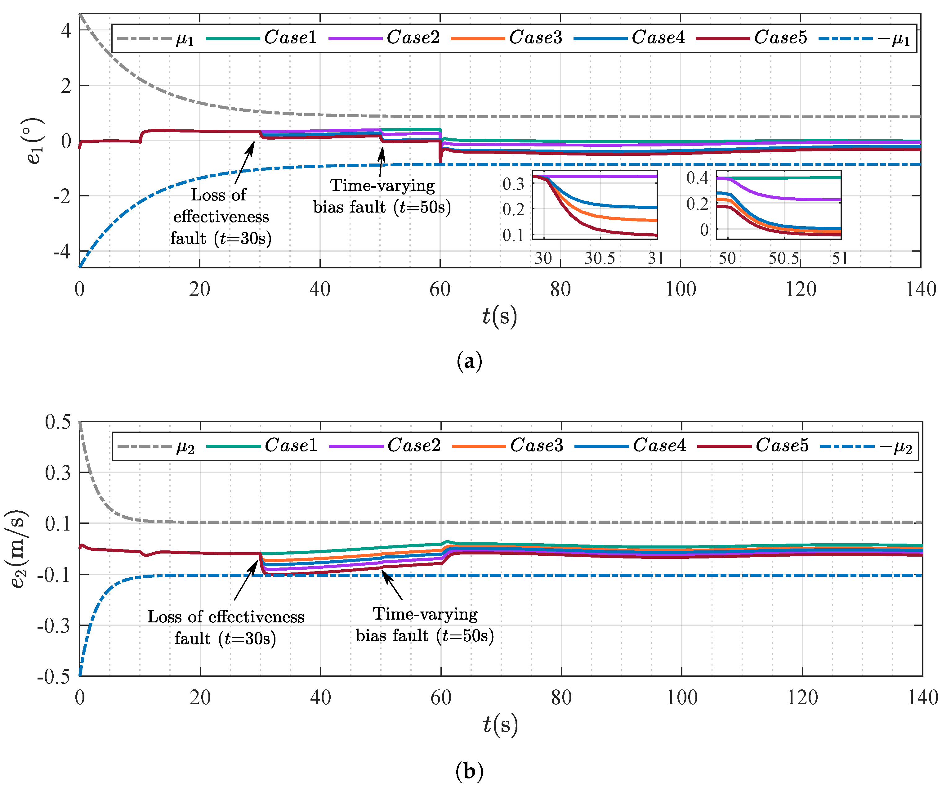
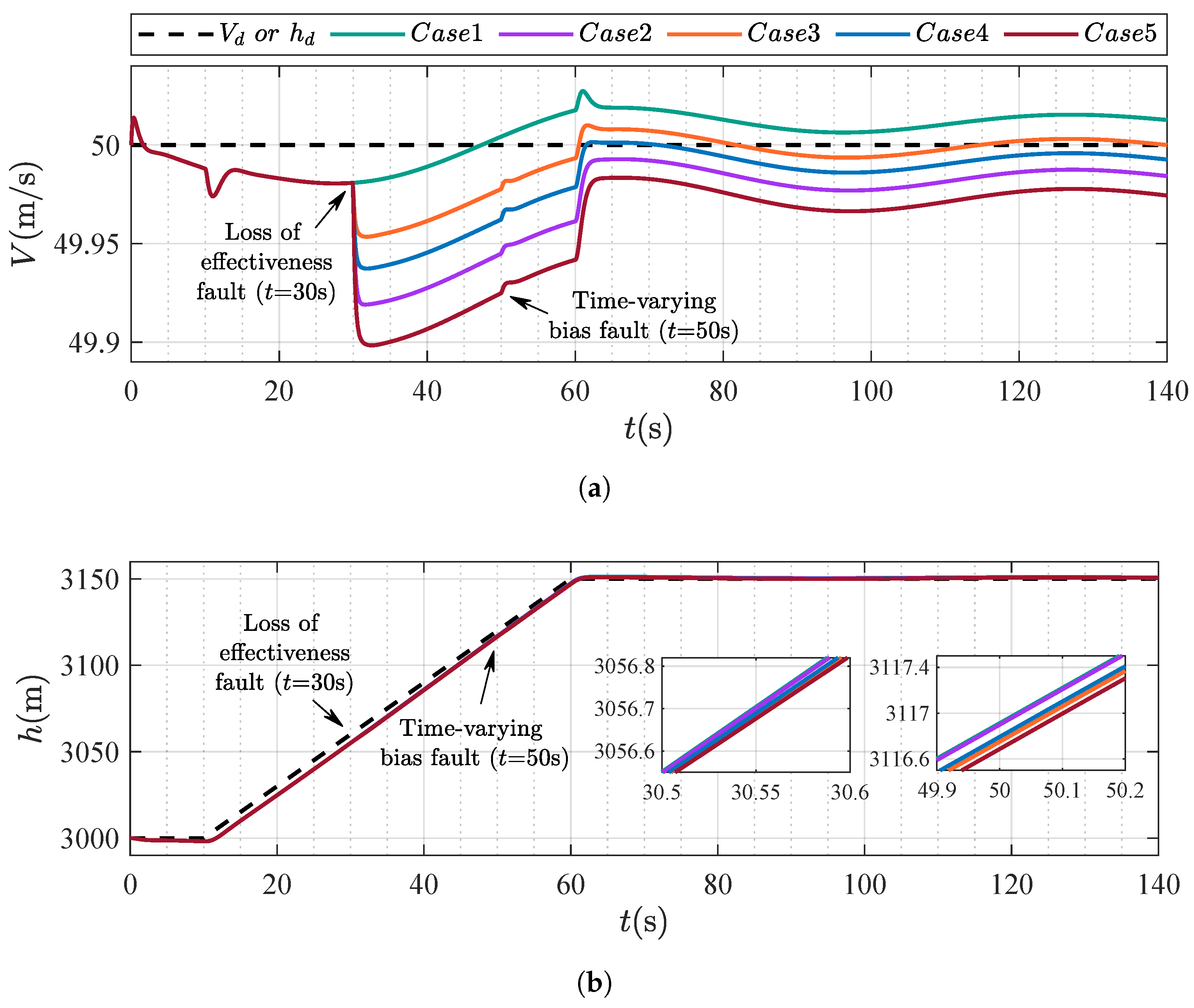
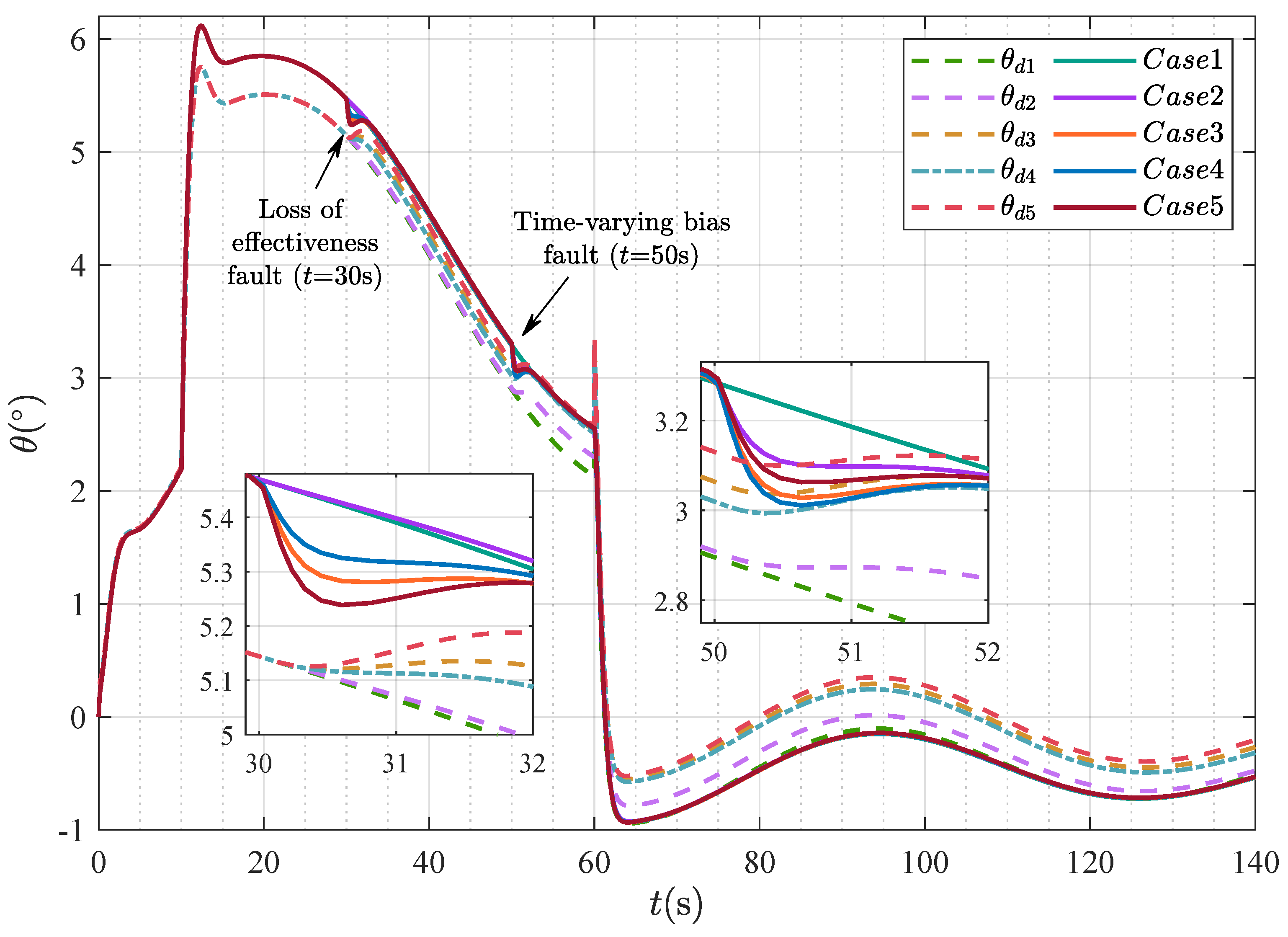
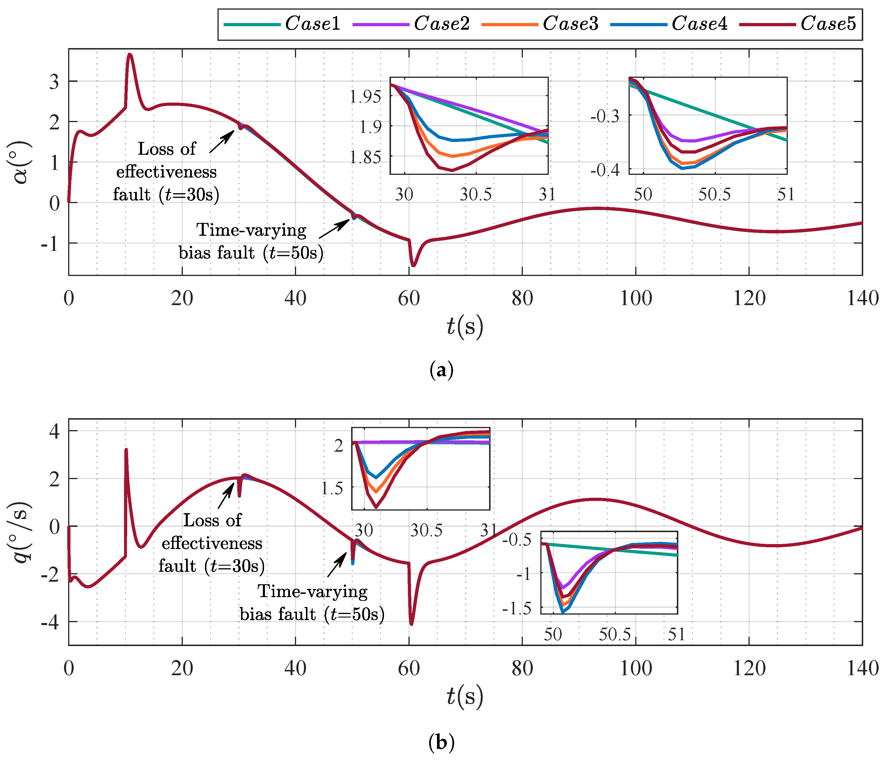
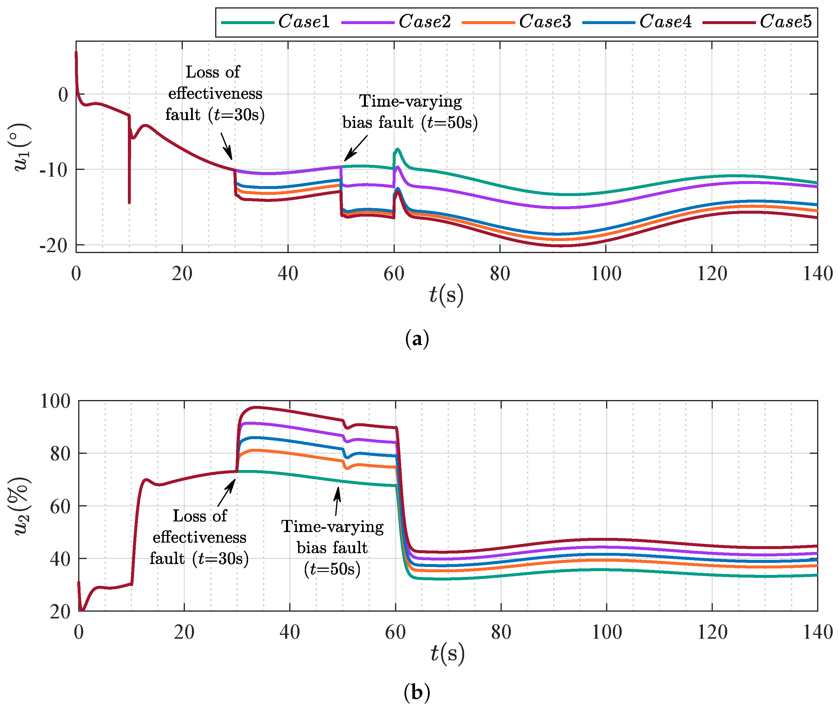
4.1. Scenario 1: Robustness Validation Under Diverse Actuator Fault Conditions

To validate the controller’s robustness and generalization capability under diverse operating conditions, numerical simulations are performed across multiple actuator fault cases (see the configuration details in

Table 4. The actuator fault conditions.

Case	Loss of Effectiveness	Time-Varying Bias
Case1	${\lambda }_1={\lambda }_2=1$	$r_1=r_2=0$
Case2	$\left\{\begin{array}{cc}{\lambda }_1={\lambda }_2=1,\hfill & \hfill t<30 \mathrm{s}\hfill \\ {\lambda }_1=0.8,{\lambda }_2=1,\hfill & \hfill t⩾30 \mathrm{s}\hfill \end{array}\right.$	$\left\{\begin{array}{cc}{r}_1=r_2=0,\hfill & \hfill t<50 \mathrm{s}\hfill \\ \hfill r_1=r_2=1,10u_1^{*}=u_2^{*}=0.5cos\left(0.01t\right),\hfill & \hfill t⩾50 \mathrm{s}\hfill \end{array}\right.$
Case3	$\left\{\begin{array}{cc}{\lambda }_1={\lambda }_2=1,\hfill & \hfill t<30 \mathrm{s}\hfill \\ {\lambda }_1=0.9,{\lambda }_2=0.8,\hfill & \hfill t⩾30 \mathrm{s}\hfill \end{array}\right.$	$\left\{\begin{array}{cc}{r}_1=r_2=0,\hfill & \hfill t<50 \mathrm{s}\hfill \\ r_1=r_2=1,10u_1^{*}=u_2^{*}=0.6cos\left(0.01t\right),\hfill & \hfill t⩾50 \mathrm{s}\hfill \end{array}\right.$
Case4	$\left\{\begin{array}{cc}{\lambda }_1={\lambda }_2=1,\hfill & \hfill t<30 \mathrm{s}\hfill \\ {\lambda }_1={\lambda }_2=0.85,\hfill & \hfill t⩾30 \mathrm{s}\hfill \end{array}\right.$	$\left\{\begin{array}{cc}{r}_1=r_2=0,\hfill & \hfill t<50 \mathrm{s}\hfill \\ r_1=r_2=1,10u_1^{*}=u_2^{*}=0.7cos\left(0.01t\right),\hfill & \hfill t⩾50 \mathrm{s}\hfill \end{array}\right.$
Case5	$\left\{\begin{array}{cc}{\lambda }_1={\lambda }_2=1,\hfill & \hfill t<30 \mathrm{s}\hfill \\ {\lambda }_1={\lambda }_2=0.75,\hfill & \hfill t⩾30 \mathrm{s}\hfill \end{array}\right.$	$\left\{\begin{array}{cc}{r}_1=r_2=0,\hfill & \hfill t<50 \mathrm{s}\hfill \\ r_1=r_2=1,10u_1^{*}=u_2^{*}=0.5cos\left(0.01t\right),\hfill & \hfill t⩾50 \mathrm{s}\hfill \end{array}\right.$

). Meanwhile, the specified parameters and the controller parameters of the proposed method are: ${\eta }_1={\eta }_2=0.06,c_1=8,c_2=0.2,k_1=15,k_2=5,{\delta }_{11}={\delta }_{21}=100,{\delta }_{12}=99.95,{\delta }_{22}=100.1,{\mu }_{1o}=4.58,{\mu }_{1\infty }=0.86,{\mu }_{2o}=0.5,{\mu }_{2\infty }=0.104,{\kappa }_1=0.1,{\kappa }_2=0.4,k_p=0.018,k_i=1\times {10}^{-5},w_1=w_2=0.2.$

Figure 4, Figure 5, Figure 6, Figure 7, Figure 8 and Figure 9 illustrate the simulation results, where the transient responses at 10 s and 60 s correlate with both the target altitude trajectory switching and the concurrent wing deformation, with the latter being the dominant contributor.

The results of the tracking errors for diverse fault conditions are shown in Figure 4. It is evident that the pitch angle error $e_1$ remains below ${0.44}^{\circ }$, while the velocity tracking error $e_2$ maintains a maximum deviation of $0.1 \mathrm{m}/\mathrm{s}$ ($0.2\%$ relative error) throughout the morphing process, strictly confined within the prescribed performance envelopes defined by ${\mu }_1\left(t\right)=(4.58-0.86)exp(-0.1t)+0.86$ and ${\mu }_2\left(t\right)=(0.5-0.104)exp(-0.4t)+0.104$.

The trajectory tracking curves are shown in Figure 5 and Figure 6. Figure 5a demonstrates that fault severity directly impacts velocity tracking accuracy, particularly at the 30 s loss of effectiveness fault. While altitude tracking remains consistent across all conditions (Figure 5b), pitch angle tracking exhibits distinct variations (Figure 6). Pitch angle curves align pre-deformation but deviate during deformation, later converging to the fault-free reference (Case 1). Actuator faults induce a transient pitch angle reduction, followed by a 0.33-s delay in reference signal adjustment and a 2-s recovery period for the actual value.

Figure 7 presents the curves of attack angle and pitch angle rate. The curves maintain consistency across fault conditions except during brief post-fault transients. Notably, the attack angle recovers within 1 s and the pitch angle rate achieves faster restoration in $0.5 \mathrm{s}$. Figure 8 shows the state trajectory of the sliding mode surface. Figure 9 displays unmanned MFV control inputs: $u_1$ ($-{20}^{\circ }$–$5^{\circ }$) and $u_2$ ($20$–$100\%$) conforming to operational specifications. The severity of faults exhibits a positive correlation with deviations from the Case 1. Furthermore, at the 30 s mark, the magnitude of $e_1,V,s_1$ and $u_1$ are associated with ${\lambda }_2$, while $e_2,\theta ,\alpha ,q,s_2$ and $u_1$ correlate with ${\lambda }_2$, which can also be confirmed in Figure 5a and Figure 6, Figure 7, Figure 8 and Figure 9. At 50 s, the $\theta ,\alpha ,q,s_1,u_1$ demonstrate strong correlation with $u_1^{*}$ and $u_2^{*}$, consistent with observations in Figure 6, Figure 7, Figure 8a and Figure 9a.

As mentioned previously, the simulation results validate that the designed controllers exhibit robustness and adaptability under various abrupt actuator faults. The fault-induced transient response manifests as an immediate pitch angle reduction, a 0.33-s reference-signal adaptation latency, and full-state recovery within 2 s, while trajectory tracking errors remain strictly bounded within prescribed performance envelopes, confirming enhanced transient performance and fault-tolerance capabilities. The proposed method enables quantifiable regulation of dynamic characteristics under concurrent actuator failures and composite disturbances.

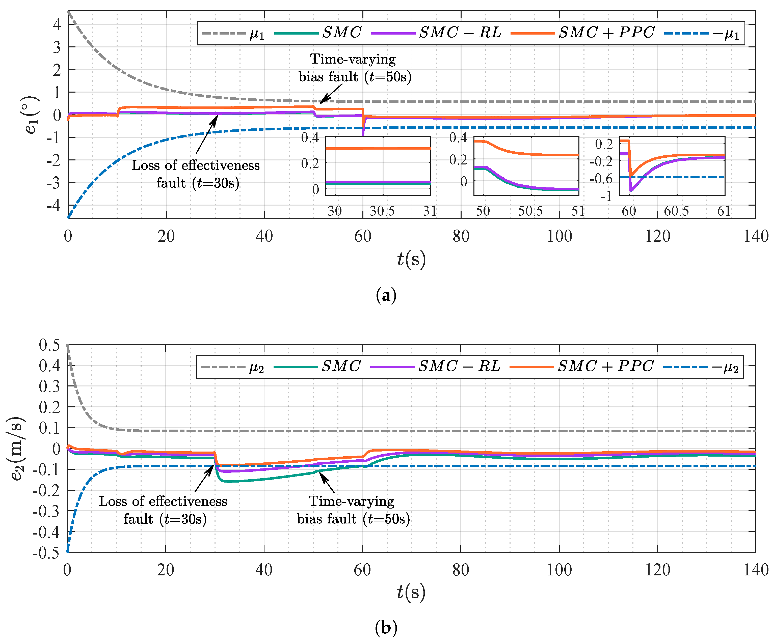
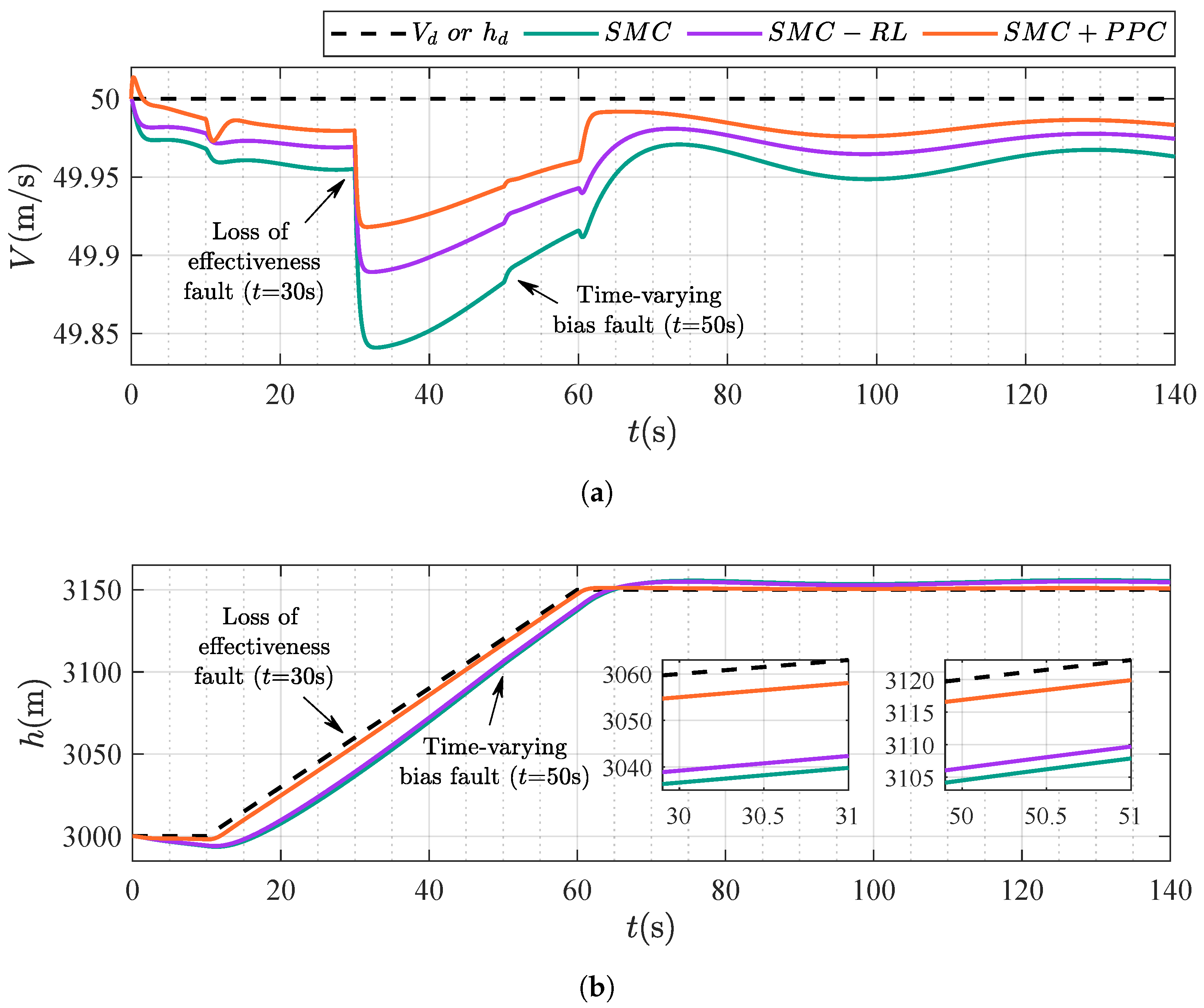
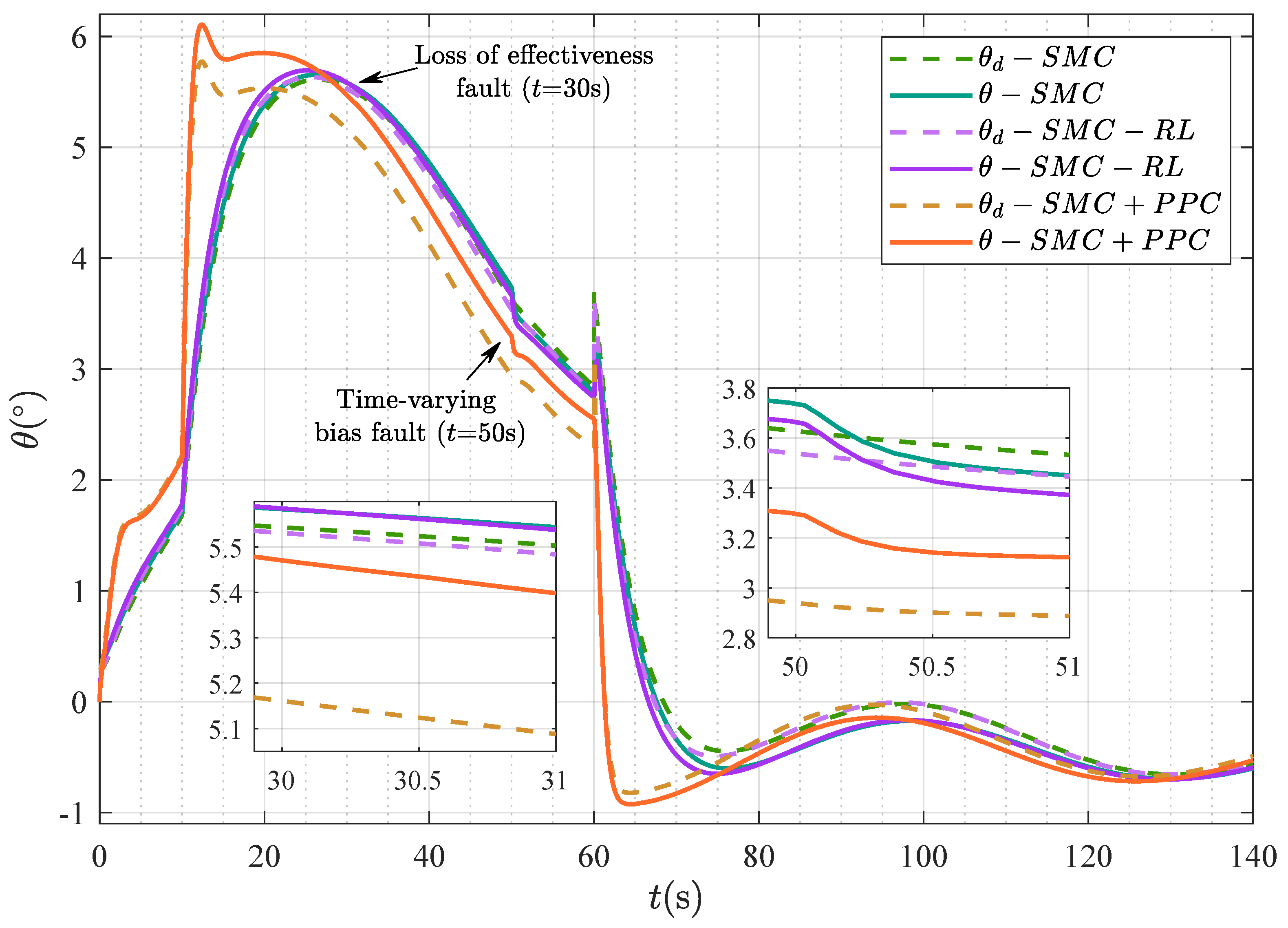
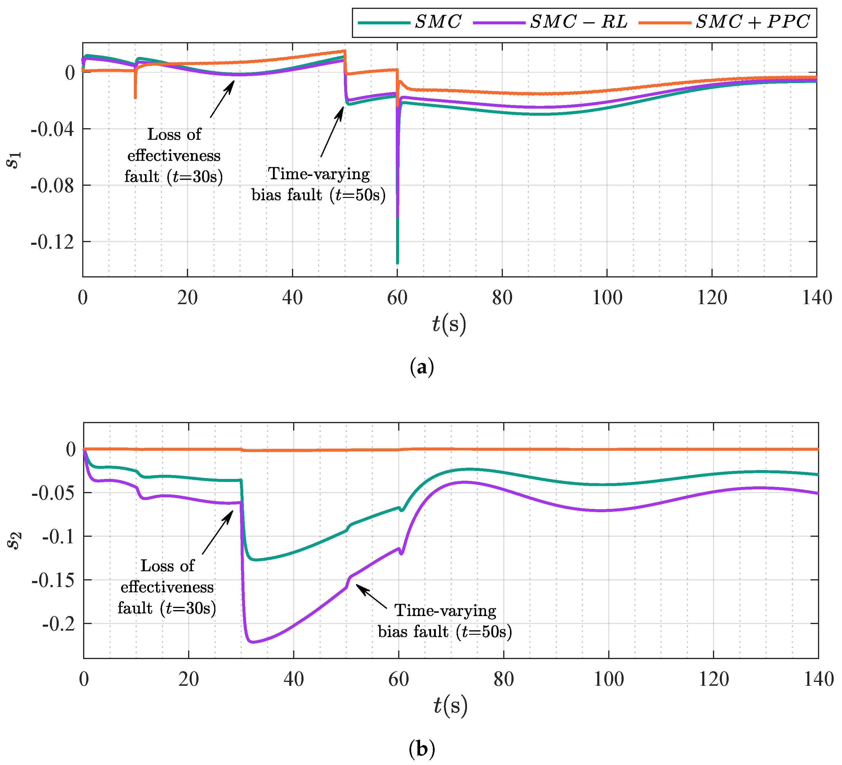
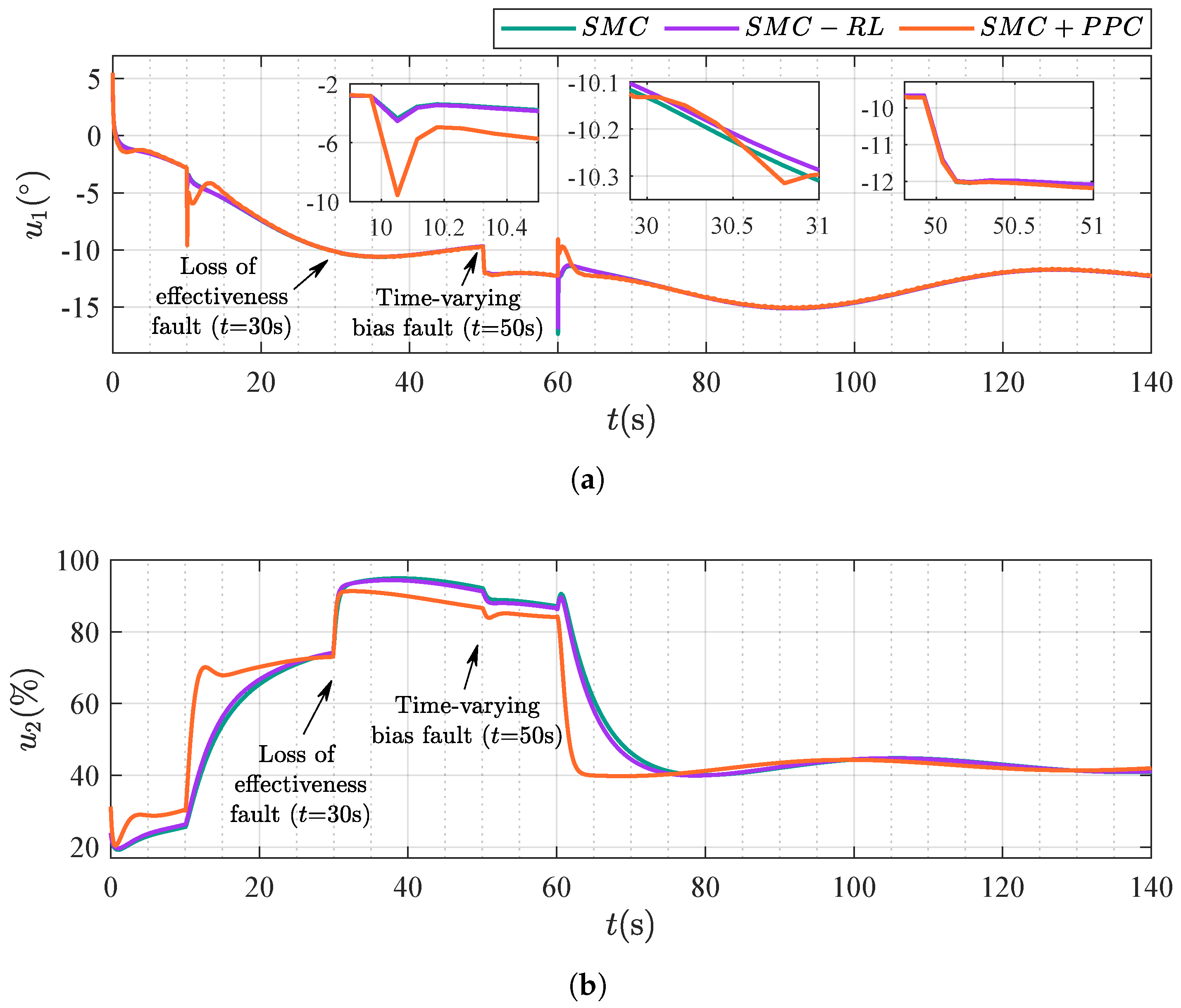
4.2. Scenario 2: Comparison Between Different Control Strategies

To better demonstrate the superiority of the proposed controller, a sliding mode controller (“SMC”) and a reaching law-based sliding mode controller (“SMC-RL”) are introduced for comparison. Similar to the proposed control strategy (“SMC+PPC”), the above two comparative methods also use the saturation function instead of the sign function to mitigate the sliding mode chattering phenomenon.

The unified fault condition is configured as follows:

• $\lambda =\mathrm{diag}\{0.8,1\}$ when $t⩾30$ s
• $r_1=r_2=1$ with $u_1^{*}=0.05cos\left(0.01t\right)$ and $u_2^{*}=0.5cos\left(0.01t\right)$ when $t⩾50$ s

The specified parameters and controller parameters of comparison strategies are shown in

Table 5. The specified parameters and the controller parameters of comparison strategies.

Methods	Parameters
SMC	$c_1=0.8,c_2=10,k_1=2.5,k_2=10,k_p=0.004,k_i=1\times {10}^{-5},w_1=w_2=0.2.$
SMC-RL	${ϵ}_1=0.1,{ϵ}_2=0.06,c_1=2,c_2=8,k_1=3.5,k_2=12,k_p=0.0045,k_i=1\times {10}^{-5},w_1=w_2=0.2.$
SMC+PPC	${\eta }_1={\eta }_2=0.06,c_1=12,c_2=0.2,k_1=15,k_2=5,{\delta }_{11}={\delta }_{21}=100,{\delta }_{12}=99.95,{\delta }_{22}=100.1,{\mu }_{1o}=4.58,{\mu }_{1\infty }=0.57,{\mu }_{2o}=0.5,{\mu }_{2\infty }=0.084,{\kappa }_1=0.1,{\kappa }_2=0.4,k_p=0.018,k_i=1\times {10}^{-5},w_1=w_2=0.2.$

, where ${ϵ}_1$ and ${ϵ}_2$ represent the reaching law parameters.

Figure 10, Figure 11, Figure 12, Figure 13, Figure 14 and Figure 15 illustrate the simulation results, where the transient dynamics at 10 s and 60 s due to wing deformation during target altitude trajectory updates.

Figure 10 compares tracking errors across control strategies, while trajectory tracking performance is detailed in Figure 11 and Figure 12. A quantitative analysis reveals that the “SMC+PPC” strategy exclusively maintains both velocity and pitch angle tracking errors within the prescribed performance envelope, with the pitch angle error $e_1$ strictly bounded below ${0.354}^{\circ }$ and the velocity error $e_2$ exhibiting a maximum deviation of $0.082 \mathrm{m}/\mathrm{s}$ ($0.164\%$ relative error) throughout the morphing process. Although the “SMC+PPC” demonstrates a slightly larger $e_1$ during the wing deformation compared to alternative methods, this discrepancy does not significantly compromise overall system performance. The “SMC-RL” is a little better than the “SMC”, which can also be proved in Figure 11 and Figure 12.

Figure 13 presents the curves of attack angle and pitch angle rate. The morphing initiation/termination phases induce significantly amplified angular deviations compared to baseline controllers, with peak attack angle and pitch angle rate excursions reaching $3.{59}^{\circ }$ and $10.{14}^{\circ }$/s at 10 s and minimum negative values of $-1.{57}^{\circ }$ and $-4.{14}^{\circ }$/s at 60 s. This unique behavior arises from the synergy between “SMC+PPC”’s enhanced disturbance rejection and constraint enforcement. Figure 14 shows the state trajectory of the sliding mode surface, which indicates that the “SMC+PPC” has the smallest sliding surface variation and the best robustness. The control inputs of the unmanned MFV are depicted in Figure 15, and it can be found from Figure 12 and Figure 15a that compared with the other two methods, the “SMC+PPC” has faster responses to the wing deformation and actuator faults.

To summarize, the simulations demonstrate the proposed “SMC+PPC” strategy’s superior fault tolerance in unmanned MFV control, achieving precise pitch angle and velocity tracking. By strategically allowing transient pitch deviations during wing deformation, the method achieves 65.2–73.1% faster disturbance recovery than “SMC” through coordinated error suppression. The proposed mechanism enables fast actuator failure recovery while maintaining stable flight dynamics, even under disturbances.

5. Conclusions

This article investigates the prescribed performance sliding mode fault-tolerant control problem for the unmanned MFV under actuator faults and composite disturbances during wing deformation. The proposed scheme systematically decouples the coupled dynamics into attitude and velocity subsystems, simplifying control synthesis while explicitly addressing fault tolerance. The constrained tracking errors are transformed into unconstrained variables through projection operators to facilitate controller design. Prescribed performance sliding mode fault-tolerant controllers are developed for each subsystem, ensuring transient response conformity to performance constraints while maintaining steady-state precision. Extensive numerical simulations validate the framework’s capability to maintain flight stability and tracking precision under simultaneous actuator faults and composite disturbances during morphing maneuvers. However, this article focuses on quasi-static deformation regimes under idealized simulation conditions, intentionally excluding real-world uncertainties such as sensor noise and actuator bandwidth constraints. Future efforts will prioritize finite-time control synthesis, adaptive multi-model architectures for dynamic morphing, and hardware-in-the-loop validation to bridge the simulation-to-reality gap, ultimately enhancing the framework’s applicability to agile maneuvers and physical deployment.

References

1. Ajaj, R.M.; Jankee, G.K. The transformer aircraft: A multi-mission unmanned aerial vehicle capable of symmetric and asymmetric span morphing. Aerosp. Sci. Technol. 2018, 76, 512–522. [Google Scholar] [CrossRef]
2. Ran, M.; Wang, C.; Liu, H.; Wang, W.; Lyu, J. Research status and future development of morphing aircraft control technology. Acta Aeronaut. Astronaut. Sin. 2022, 43, 424–441. (In Chinese) [Google Scholar] [CrossRef]
3. Parancheerivilakkathil, M.S.; Pilakkadan, J.S.; Ajaj, R.M.; Amoozgar, M.; Asadi, D.; Zweiri, Y.; Friswell, M.I. A review of control strategies used for morphing aircraft applications. Chin. J. Aeronaut. 2024, 37, 436–463. [Google Scholar] [CrossRef]
4. Yan, B.; Li, Y.; Dai, P.; Liu, S. Aerodynamic analysis, dynamic modeling, and control of a morphing aircraft. J. Aerosp. Eng. 2019, 32, 04019058. [Google Scholar] [CrossRef]
5. Bai, B.; Dong, C. Modeling and LQR switch control of morphing aircraft. In Proceedings of the 2013 6th International Symposium on Computational Intelligence and Design, Hangzhou, China, 28–29 October 2013; pp. 148–151. [Google Scholar] [CrossRef]
6. Fan, W.; Liu, H.H.T.; Kwong, R.H.S. Gain-scheduling control of flexible aircraft with actuator saturation and stuck faults. J. Guid. Control Dyn. 2017, 17, 497–502. [Google Scholar] [CrossRef]
7. Li, Y.; Wang, Y.; Liu, L. Longitudinal adaptive control of morphing aircraft based on guardian maps theory. Int. J. Aeronaut. Space Sci. 2025. [Google Scholar] [CrossRef]
8. Cai, G.; Yang, Q.; Mu, C.; Li, X. Design of linear parameter-varying controller for morphing aircraft using inexact scheduling parameters. IET Control Theory Appl. 2022, 17, 493–503. [Google Scholar] [CrossRef]
9. Cai, G.; Wu, T.; Hao, M.; Liu, H.; Zhou, B. Dynamic event-triggered gain-scheduled H control for a polytopic LPV model of morphing aircraft. IEEE Trans. Aerosp. Electron. Syst. 2025, 61, 93–106. [Google Scholar] [CrossRef]
10. Yuan, L.; Wang, L.; Xu, J. Adaptive fault-tolerant controller for morphing aircraft based on the L2 gain and a neural network. Aerosp. Sci. Technol. 2022, 132, 107985. [Google Scholar] [CrossRef]
11. Wu, K.; Zhang, P.; Wu, H. A new control design for a morphing UAV based on disturbance observer and command filtered backstepping techniques. Sci. China Technol. Sci. 2019, 62, 1845–1853. [Google Scholar] [CrossRef]
12. Gong, L.; Wang, Q.; Dong, C. Disturbance rejection control of morphing aircraft based on switched nonlinear systems. Nonlinear Dyn. 2019, 96, 975–995. [Google Scholar] [CrossRef]
13. Meng, F.; Wang, T.; Chen, G. Prescribed performance-based active anti-disturbance backstepping control for morphing aircraft. Aerosp. Sci. Technol. 2024, 152, 109386. [Google Scholar] [CrossRef]
14. Shi, R.; Song, J. Dynamics and control for an in-plane morphing wing. Aircr. Eng. Aerosp. Technol. 2013, 85, 24–31. [Google Scholar] [CrossRef]
15. Huang, R.; Hu, H.; Zhao, Y. Single-input/single-output adaptive flutter suppression of a three-dimensional aeroelastic system. J. Guid. Control Dyn. 2012, 35, 659–665. [Google Scholar] [CrossRef]
16. Xu, S.; Guan, Y.; Wei, C.; Xu, H. Broad learning system-based model-free adaptive robust control for hypersonic morphing aircraft with appointed-time prescribed performance. Eng. Appl. Artif. Intell. 2025, 143, 109962. [Google Scholar] [CrossRef]
17. Luo, M.; Gao, M.; Cai, G. Delayed full-state feedback control of airfoil flutter using sliding mode control method. J. Fluids Struct. 2016, 61, 262–273. [Google Scholar] [CrossRef]
18. Wang, Q.; Wang, W.; Suzuki, S.; Namiki, A.; Liu, H.; Li, Z. Design and implementation of UAV velocity controller based on reference model sliding mode control. Drones 2023, 7, 130. [Google Scholar] [CrossRef]
19. Liu, X.; Xu, Y.; Luo, J. An asymmetrically variable wingtip anhedral angles morphing aircraft based on incremental sliding mode control: Improving lateral maneuver capability. Chin. J. Aeronaut. 2024, 38, 103166. [Google Scholar] [CrossRef]
20. Wei, C.; Luo, J.; Yin, Z. A review of prescribed performance control for spacecraft attitude. J. Astronaut. 2019, 40, 1167–1176. (In Chinese) [Google Scholar] [CrossRef]
21. Ghanooni, P.; Habibi, H.; Yazdani, A.; Wang, H.; MahmoudZadeh, S.; Ferrara, A. Prescribed performance control of a robotic manipulator with unknown control gain and assigned settling time. ISA Trans. 2023, 145, 330–354. [Google Scholar] [CrossRef]
22. Vo, A.T.; Truong, T.N.; Kang, H.J. Fixed-time RBFNN-based prescribed performance control for robot manipulators: Achieving global convergence and control performance improvement. Mathematics 2023, 11, 2307. [Google Scholar] [CrossRef]
23. Wu, Q.; Zhu, Q. Prescribed performance fault-tolerant attitude tracking control for UAV with actuator faults. Drones 2024, 8, 204. [Google Scholar] [CrossRef]
24. Yuan, L.; Zheng, J.; Wang, X.; Ma, L. Attitude control of a mass-actuated fixed-wing UAV based on adaptive global fast terminal sliding mode control. Drones 2024, 8, 305. [Google Scholar] [CrossRef]
25. Zhao, S.; Li, X.; Bu, X.; Zhang, D. Prescribed performance tracking control for hypersonic flight vehicles with model uncertainties. Int. J. Aerosp. Eng. 2019, 2019, 1–11. [Google Scholar] [CrossRef]
26. Hu, Q.; Shao, X.; Guo, L. Adaptive fault-tolerant attitude tracking control of spacecraft with prescribed performance. IEEE/ASME Trans. Mechatronics 2018, 23, 331–341. [Google Scholar] [CrossRef]
27. Yin, Z.; Wang, B.; Xiong, R.; Xiang, Z.; Liu, L.; Fan, H.; Xue, C. Attitude tracking control of hypersonic vehicle based on an improved prescribed performance dynamic surface control. Aeronaut. J. 2023, 128, 875–895. [Google Scholar] [CrossRef]
28. Ding, Y.; Yue, X.; Chen, G.; Si, J. Review of control and guidance technology on hypersonic vehicle. Chin. J. Aeronaut. 2021, 35, 1–18. [Google Scholar] [CrossRef]
29. Wen, L.; Tao, G.; Jiang, B.; Chen, W. Adaptive compensation of persistent actuator failures using control-separation-based LQ design. IEEE Trans. Syst. Man Cybern. Syst. 2019, 51, 5030–5045. [Google Scholar] [CrossRef]
30. Chao, D.; Qi, R.; Jiang, B. Adaptive fault-tolerant attitude control for hypersonic reentry vehicle subject to complex uncertainties. J. Frankl. Inst. 2022, 359, 5458–5487. [Google Scholar] [CrossRef]
31. Liu, S.; Whidborne, J.F. Observer-based incremental backstepping sliding-mode fault-tolerant control for blended-wing-body aircrafts. Neurocomputing 2021, 464, 546–561. [Google Scholar] [CrossRef]
32. Liang, X.; Wang, Q.; Hu, C.; Dong, C. Fixed-time observer based fault tolerant attitude control for reusable launch vehicle with actuator faults. Aerosp. Sci. Technol. 2020, 107, 106314. [Google Scholar] [CrossRef]
33. Liu, C.; Jiang, B.; Song, X.; Zhang, S. Fault-tolerant control allocation for over-actuated discrete-time systems. J. Frankl. Inst. 2015, 352, 2297–2313. [Google Scholar] [CrossRef]
34. Khan, S.; Grigorie, T.; Botez, R.; Mamou, M.; Mébarki, Y. Fuzzy logic-based control for a morphing wing tip actuation system: Design, numerical simulation, and wind tunnel experimental testing. Biomimetics 2019, 4, 65. [Google Scholar] [CrossRef] [PubMed]
35. Wang, Y.; Xu, J.; Huang, S.; Lin, Y.; Jiang, J. Computational study of axisymmetric divergent bypass dual throat nozzle. Aerosp. Sci. Technol. 2019, 86, 177–190. [Google Scholar] [CrossRef]
36. Yan, B.; Dai, P.; Liu, R.; Xing, M.; Liu, S. Adaptive super-twisting sliding mode control of variable sweep morphing aircraft. Aerosp. Sci. Technol. 2019, 92, 198–210. [Google Scholar] [CrossRef]
37. Yin, M. Coordinated Control of Deformation and Flight for Morphing Aircraft. Ph.D. Thesis, Nanjing University of Aeronautics and Astronautics, Nanjing, China, 2015. [Google Scholar]
38. Zheng, W. Research on Nonlinear Control Method of Morphing Aircraft. Master’s Thesis, Harbin Institude of Technology, Harbin, China, 2022. [Google Scholar]
Figure 1. The control framework of the proposed method.
Drones 09 00292 g001
Figure 2. An unmanned MFV in the process of wingspan deformation [9].
Drones 09 00292 g002
Figure 3. The variation in wingspan deformation rate over time.
Drones 09 00292 g003
Figure 4. Comparison curves of tracking errors for diverse fault conditions: (a) pitch angle tracking error; (b) velocity tracking error.
Drones 09 00292 g004
Figure 5. Comparison curves of tracking trajectories for diverse fault conditions: (a) velocity tracking curve; (b) altitude tracking curve.
Drones 09 00292 g005
Figure 6. Comparison curves of tracking pitch angle θ for diverse fault conditions.
Drones 09 00292 g006
Figure 7. Comparison curves of attack angle α and pitch angle rate q for diverse fault conditions: (a) attack angle α ; (b) pitch angle rate q.
Drones 09 00292 g007
Figure 8. Comparison curves of sliding surface changes for diverse fault conditions: (a) sliding mode surface changes of the attitude subsystem; (b) sliding mode surface changes of the velocity subsystem.
Drones 09 00292 g008
Figure 9. Comparison curves of inputs for diverse fault conditions: (a) elevator deflection angle; (b) throttle opening.
Drones 09 00292 g009
Figure 10. Comparison curves of tracking errors for different control strategies: (a) pitch angle tracking error; (b) velocity tracking error.
Drones 09 00292 g010
Figure 11. Comparison curves of tracking trajectories for different control strategies: (a) velocity tracking curve; (b) altitude tracking curve.
Drones 09 00292 g011
Figure 12. Comparison curves of tracking pitch angle θ for different control strategies.
Drones 09 00292 g012
Figure 13. Comparison curves of attack angle α and pitch angle rate q for different control strategies: (a) attack angle α ; (b) pitch angle rate q.
Drones 09 00292 g013
Figure 14. Comparison curves of sliding mode surface changes for different control strategies: (a) sliding mode surface changes of the attitude subsystem; (b) sliding mode surface changes of the velocity subsystem.
Drones 09 00292 g014
Figure 15. Comparison curves of inputs for different control strategies: (a) elevator deflection angle; (b) throttle opening.
Drones 09 00292 g015