Robust UAV Target Tracking Algorithm Based on Saliency Detection

Abstract

Due to their high efficiency and real-time performance, discriminant correlation filtering (DCF) trackers have been widely applied in unmanned aerial vehicle (UAV) tracking. However, the robustness of existing trackers is still poor when facing complex scenes, such as background clutter, occlusion, camera motion, and scale variations. In response to this problem, this paper proposes a robust UAV target tracking algorithm based on saliency detection (SDBCF). Using saliency detection methods, the DCF tracker is optimized in three aspects to enhance the robustness of the tracker in complex scenes: feature fusion, filter-model construct, and scale-estimation methods improve. Firstly, this article analyzes the features from both spatial and temporal dimensions, evaluates the representational and discriminative abilities of different features, and achieves adaptive feature fusion. Secondly, this paper constructs a dynamic spatial regularization term using a mask that fits the target, and integrates it with a second-order differential regularization term into the DCF framework to construct a novel filter model, which is solved using the ADMM method. Next, this article uses saliency detection to supervise the aspect ratio of the target, and trains a scale filter in the continuous domain to improve the tracker’s adaptability to scale variations. Finally, comparative experiments were conducted with various DCF trackers on three UAV datasets: UAV123, UAV20L, and DTB70. The DP and AUC scores of SDBCF on the three datasets were (71.5%, 58.9%), (63.0%, 57.8%), and (72.1%, 48.4%), respectively. The experimental results indicate that SDBCF achieves a superior performance.

1. Introduction

In recent years, drone technology has rapidly emerged as an important tool in various fields such as intelligent video surveillance [1,2], human–computer interaction [3], aviation reconnaissance [4], precision guidance [5], military strikes [6], etc., thanks to its advantages of a small size, a low cost, and flexible movement. With the continuous expansion of drone application scenarios, its autonomous navigation and target-tracking capabilities have become key technologies for improving overall performance. Robust target tracking algorithms not only ensure the stable recognition and localization of specific targets by drones in complex environments, but also provide real-time decision support during tasks such as search and rescue and border patrol. Therefore, research on unmanned aerial vehicle target tracking technology has broad application prospects [7].

However, in the actual tracking process, due to the complexity of application scenarios and limitations of onboard platforms [8], achieving precise and robust tracking using drones still faces significant challenges. Firstly, unmanned aerial vehicles (UAVs) have strong maneuverability and flexible movements. During the execution of tracking tasks, they will face more complex and dynamic background environments, which pose certain difficulties for precise target positioning. Secondly, in certain application scenarios, drones may capture the imaging pose of targets from different angles, causing changes in the appearance of the targets and requiring trackers to have strong adaptability. In addition, rapid motion and changes in perspective can cause significant scale changes in the target during tracking, and the accuracy of scale estimation directly affects the tracking accuracy. Therefore, unmanned aerial vehicle target tracking algorithms also require the trackers to have high-scale estimation capabilities.

In recent years, scholars have conducted in-depth research and made significant progress in improving the performance of unmanned aerial vehicle target tracking algorithms. Although deep learning-based methods have demonstrated excellent performance in complex scenarios through learning the high-level semantic features of targets, their tracking accuracy is highly dependent on the training of large-scale annotated datasets, and the distribution characteristics of the training data limit the model’s generalization ability. In addition, the parameter debugging process of neural networks is relatively cumbersome. In contrast, the DCF-based method obtains the features of the target through the first frame of the image sequence and utilizes an online learning mechanism to update the target appearance model in real time, which means it can adapt to dynamic changes in the target appearance without relying on pre-trained datasets. At the same time, the number of parameters is relatively low and the physical meaning is clear. Researchers can adjust the parameters reasonably according to specific scene requirements. The above characteristics make the DCF algorithm more applicable in the field of unmanned aerial vehicle target tracking.

The core idea of a DCF-based tracker is to train a filter on the search area by minimizing the sum of squared errors between the ideal output and the actual output. Then, the filter is correlated with the search area of the next frame to obtain a response map. The position corresponding to the maximum value of the response map is the center of the target. MOSSE (Minimum Output Sum of Squared Error) [9] was the first technique to apply correlation filtering to the tracking field, converting time-domain correlation operations into frequency-domain element-wise multiplication, significantly reducing the computational complexity and achieving a tracking speed of 669 fps. This is the pioneering work of the DCF tracking algorithm. Subsequently, CSK (Circular Structure with Kernels) [10] cyclically shifted the training samples to obtain negative samples and established a relationship between correlation filtering and Fourier transform using the diagonalization of cyclic matrices in the Fourier domain, further improving the performance of the DCF tracker. Subsequently, KCF (Kernelized Correlation Filter) [11] introduced multi-channel HOG (Histogram of Oriented Gradient) features into DCF and transformed the problem of target tracking into a ridge regression problem, laying the foundation for the development of subsequent DCF tracking algorithms.

After KCF, research on DCF trackers mainly focused on fusing different features [12,13,14], establishing more robust appearance models [6,15,16], improving scale estimation strategies [17,18], optimizing model update mechanisms [9,19], and so on. Although these studies have improved the accuracy of trackers to varying degrees, there are still some issues when applied to the field of UAV target tracking, as follows: (1) UAV scenes often face highly dynamic changes and high-complexity background environments, and therefore require feature representations with higher discriminability and stronger representation capabilities. Discriminative ability refers to the ability of features to distinguish between targets and backgrounds in the spatial dimension, while representational ability refers to the ability of features to adapt to changes in the appearance of targets in the temporal dimension. However, many trackers simply stack multiple features or fuse them in fixed proportions, without exploring the spatial and temporal connections between different features and achieving the adaptive fusion of multiple features in different scenarios. Therefore, the advantages of different features cannot be fully utilized, which, to some extent, limits the performance of trackers. (2) Most existing DCF methods for improving tracker models are based on spatial and temporal regularization terms. The spatial regularization term can effectively suppress the boundary effects caused by cyclic operations, while the temporal regularization term can enhance the temporal continuity of the filter and avoid distortion of the filter model due to factors such as occlusion. Both effectively improve the performance of the tracker. However, there is still room for improvement in existing methods. The spatial regularization term does not pay enough attention to the target, making the tracker susceptible to interference from background clutter, similar objects, and other factors in complex and changing scenes. The temporal regularization term only utilizes the information of adjacent frames of the filter, without fully utilizing earlier historical information and the information of the filter change rate, which, to some extent, limits the anti-distortion ability of the tracker. (3) The improvement in scale filters achieved using the DCF algorithm mostly focuses on implementing aspect ratio adaptation, ignoring the problem of discontinuous scale resolution caused by multi-scale sampling. In some scenarios, drones need to track and aim at targets ranging from far to near, and the scale of the targets will slowly change during this process. When the target scale is scaled between two fixed scale resolutions, due to computational accuracy, the estimated scale of the filter will switch back and forth between the two scales, causing jitter in the center and frame of the target and seriously affecting the robustness of the tracker. In addition, recently, many scholars have introduced saliency detection into DCF trackers, used it to select feature channels, or used it to construct spatial regularization terms. Many studies have shown that the reasonable use of saliency information can improve the tracking accuracy of filters. However, most of these studies utilize saliency information to improve one aspect of the filter, and few scholars have introduced saliency information into multiple aspects of the filter simultaneously to integrate the performance of the tracker, resulting in the underutilization of saliency information.

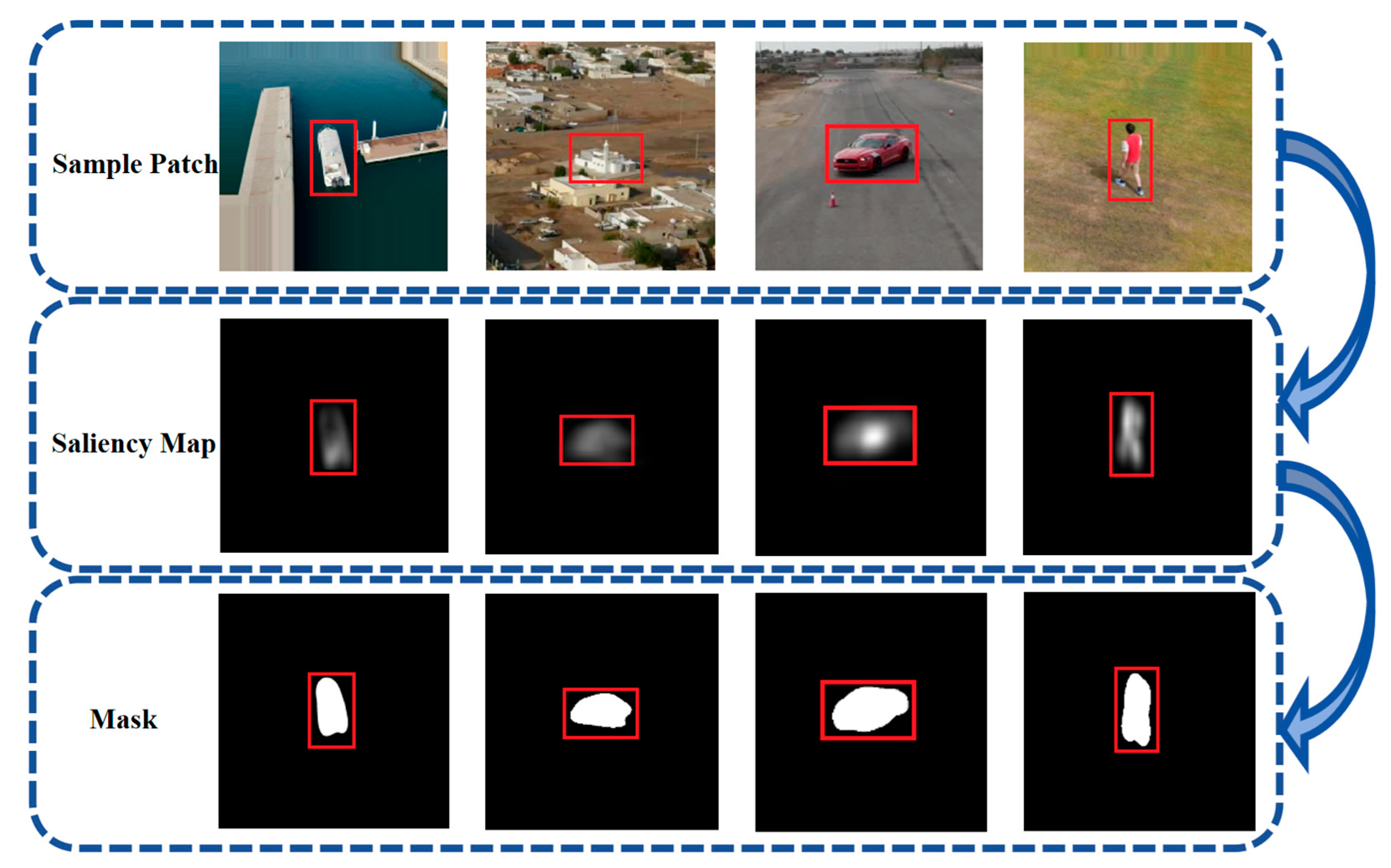
In response to the above issues, this paper proposed a robust UAV target tracking algorithm based on saliency detection (SDBCF), which integrates saliency information into multiple modules, such as feature fusion, model construction, and scale estimation, to comprehensively improve the robustness of the tracker. The main contributions of this paper are as follows:

(1)

A dynamic feature fusion scheme is proposed. Based on the saliency information and historical information of features, the discriminative and representational abilities of each feature are quantified, enabling the dynamic fusion of features in different scenarios and improving the robustness of the tracker in scenarios such as background clutter and deformation.

(2)

A robust filter model is constructed. By utilizing saliency detection, the filter model is guided to focus on learning target information in the spatial dimension, while also reasonably learning background information, which enhances the discriminative ability of the filter in scenarios such as background clutter. By utilizing second-order differential regularization terms to constrain the temporal rate of change of the filter, the robustness of the filter in scenarios such as occlusion and camera motion is improved. The use of ADMM method to solve the model improved the tracking speed.

(3)

A high-precision scale estimation strategy is proposed. The adaptive aspect ratio change in the target is achieved by using the significance detection method, and the continuous scale space is constructed by the interpolation method to estimate the continuous scale change in the target, which improves the robustness of the tracker in scale-change scenarios.

(4)

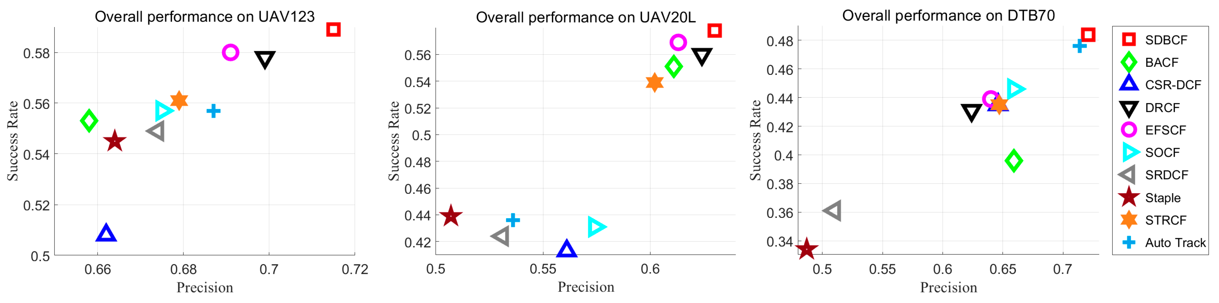
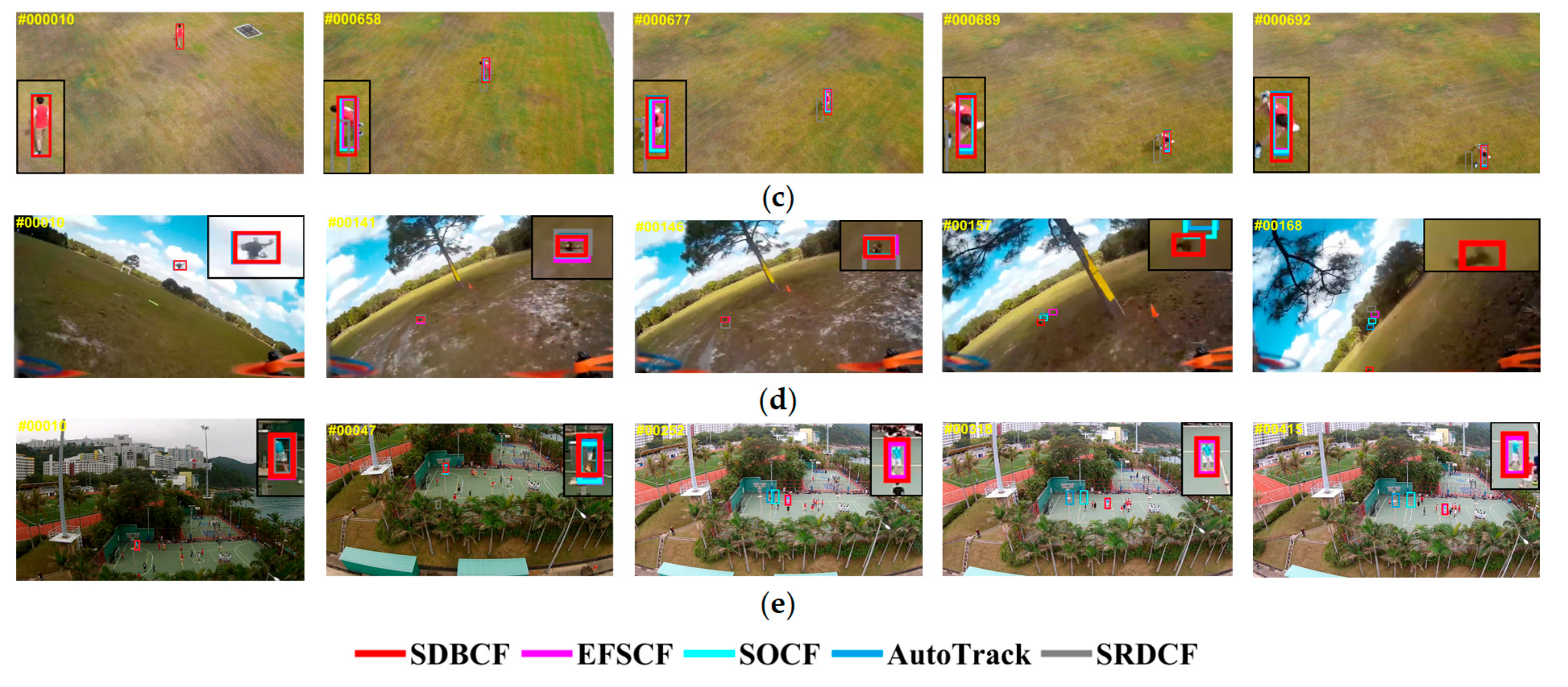
The performance of SDBCF was tested on the UAV123, UAV20L, and DTB70 datasets. The experimental results showed that the tracking accuracy and success rate of the tracker exceeded those of the existing mainstream trackers, and it exhibited superior performance in terms of various attributes, such as background clutter, occlusion, similar object interference, aspect ratio changes, scale changes, and camera motion, proving the effectiveness of the proposed method.

Next, in Section 2, this paper first reviews the research status of the DCF algorithm, and then introduces the tracking framework and specific details of SDBCF in Section 3. Section 4 presents the experimental results and an analysis of SDBCF, as well as comparative algorithms. Finally, the conclusion of this article and the outlook for the future are presented.

2. Related Work

This section provides a brief review of the most relevant DCF trackers to our work, including trackers that optimize filter models, trackers that fuse features, trackers based on saliency detection, and trackers that optimize scale estimation strategies.

In recent years, researchers have made many attempts to optimize filter models and improve the robustness of filters in complex scenarios and have achieved many impressive results. ARCF [20] adds a response graph regularization term to the DCF framework, which constrains the response graphs between adjacent frames to suppress filter distortion caused by factors such as occlusion, thereby improving the robustness of the tracker. RTSBACF [21] includes a sample suppression term based on BACF to suppress interfered-with information, and proposed a sample compensation strategy to compensate for undisturbed information, effectively reducing background interference and fully utilizing undisturbed target and background information. BAASR [22] introduces background-aware information into the objective function and develops a novel spatial regularization term. This regularization term integrates both the appearance information of the target and the reliability of the tracking results, and obtains spatial weight values through an energy function, effectively improving the tracking precision of the filter. SOCF [23] uses a spatial disturbance suppression strategy, which first utilizes the temporal information in the historical response map to detect disturbance information in the background. Then, a spatial disturbance map is constructed to suppress negative samples in the disturbance area, effectively separating the target from the background and making the filter focus more on the target itself during training. LDECF [24] proposes a dynamic sensitivity regularization term that constrains the forward-tracking and historical backtracking response of the filter between consecutive frames, making the filter more flexible. This can not only adapt to rapid changes in the target, but can also adapt to highly dynamic background environments.

The adaptive fusion of features is one of the current research hotspots in DCF algorithms, with the aim of providing a more comprehensive and accurate description of the target. LSVKSCF [25] is a new multi-expert feature fusion strategy. In this method, multiple features are randomly combined, and the target is tracked and predicted separately. The mutual overlap rate of the predicted bounding boxes and the self-overlap rate between historical frames are used to evaluate each feature, thereby achieving an adaptive fusion of features. UOT [26] uses a two-step feature compression mechanism that reduces feature dimensionality by compressing redundant features, while combining multiple compressed features based on the PSR (Peak to Sidelobe Ratio) [9] to accurately characterize the target. Zhang et al. [27] proposed a feature fusion method that first enhances the features using the PSR, making the response map smoother and the peaks more prominent. Then, different features are fused based on the enhanced response, so that the fused features can better describe the target. SCSTCF [28] uses a binary linear programming feature fusion method, which pre-set three fusion weights, fused response maps separately for each weight, and selected the weight with the minimum L2 norm of the difference between the response maps before and after fusion as the final fusion weight, improving the adaptive ability of the tracker. DSTRCFT [29] uses a multi-memory tracking framework that combines different features to track targets in parallel, and uses memory evaluation based on reliability scores to select the best memory for the final tracking results.

In order to improve the performance of trackers in complex scenes, many scholars have introduced image segmentation into the field of target tracking, which is used to learn target and non-target regions separately. Significance testing is the most common method. DRCF [30] constructs a dual regularized correlation filter tracker for saliency detection, integrating saliency information into both spatial regularization and ridge regression terms to impose stronger penalties on non-target regions. SDCS-CF [31] uses a pixel-level saliency map generation method to adjust the weights of search area features, thereby achieving robust tracking and improving resistance to background interference. Zhang et al. [32] integrated a saliency enhancement term in the DCF framework to emphasize target information, enabling the tracker to effectively highlight the target during tracking while suppressing background noise. TRSADCF [33] uses saliency information to distinguish between target and non-target regions in the response map, thereby improving the filter response in the target region. CSCF [34] combines saliency information with filters and integrates them into the DCF framework, improving the tracking performance of trackers in complex scenes such as deformation, motion blur, and background clutter.

The results of scale estimation have a significant impact on the performance of trackers. When the tracking box is too large, the template will contain too much background information; when the tracking box is too small, the template will lose some target features, making it difficult for it to fully learn the appearance of the target, ultimately leading to tracking failure. Therefore, improving the accuracy of scale estimation is also a research focus of DCF trackers. PSACF [35] uses a scale adaptive method based on probability estimation, which utilizes a Gaussian distribution model to estimate the target scale and introduces the assumption of global and local scale consistency to restore the target scale. This method can handle scale changes without using multi-scale features. He et al. [36] proposed a variable scale learning method that introduces a variable scale factor, overcoming the limitations of fixed scale factors in the commonly used multi-scale search strategies. Then, multi-scale aspect ratios compensate for the shortcomings of constant aspect ratios. By combining variable scale factors with multiple aspect ratios, a variable scale aspect ratio estimation method is implemented. FAST [37] proposed a scale search scheme that integrates Average Peak Correlation Energy (APCE) [38] into the displacement filter framework to achieve robust and accurate scale estimation. MCPF [37] utilizes a particle sampling strategy for the scale estimation of targets, effectively addressing the problem of large-scale variations. Chen et al. [39] proposed a two-dimensional scale space search method that detects the width and height of the target separately, improving the performance of the tracker in scenarios with large-scale and vertical/horizontal changes in the target.

Compared to the existing research, the uniqueness of SDBCF lies in its deep integration of the complexity and variability of drone target tracking scenarios, and the implementation of the collaborative optimization of multiple modules of the tracker through saliency methods, thereby comprehensively enhancing the robustness of the tracker in complex environments. Specifically, in the feature fusion module, SDBCF fully explores the spatial and temporal dimensions of each feature, achieving the adaptive fusion of multiple features, and thereby enhancing the comprehensiveness and adaptability of feature representation. In terms of model construction, SDBCF effectively suppresses interference from non-target areas using saliency information, and by imposing constraints on the temporal rate of change in the filter, it effectively avoids model distortion and constructs a more robust filter model. In terms of scale estimation, the SDBCF algorithm not only adapts to changes in the aspect ratio of the target, but also accurately estimates continuous changes in the target scale, significantly improving the accuracy and flexibility of scale estimation.

3. Proposed Method

In this section, we first review the basic framework of the DCF tracker. Then, we provide a detailed introduction to the SDBCF we propose.

3.1. Conventional Correlation Filter Learning

3.1.1. Displacement Filter

Traditional DCF trackers typically consist of a displacement filter and a scale filter. Firstly, the displacement filter is used to estimate the target position, and then the scale filter is used to estimate the target scale. Our displacement filter is optimized based on SRDCF. SRDCF is typically trained by minimizing the objective function in Equation (1):

$$\epsilon (f)={\displaystyle \frac{1}{2}}{‖{\displaystyle \sum _{d=1}^D{x}_t^d⊚f_t^d}-y‖}_2^2+{\displaystyle \frac{1}{2}}{{\displaystyle \sum _{d=1}^D‖w_s\odot f_t^d‖}}_2^2$$

(1)

$x_t^d\in R^{M\times N}(d=1,2,\dots ,D)$ is the sample feature of size $M\times N$ extracted in frame $t$, $D$ represents the number of feature channels, $y\in R^{M\times N}$ is the expected Gaussian shape response, $y\in R^{M\times N}$ represents the filter of the $d-th$ channel trained in the $t-th$ frame, and $⊚$ represents the discrete cyclic correlation operator. $1/2{\displaystyle {\sum }_{d=1}^D{‖w_s\odot f_t^d‖}_2^2}$ is the spatial regularization term, $w_s$ is the weight of the bowl-shaped static spatial regularization term, and $\odot$ represents the Hadamard product.

3.1.2. Scale Filter

Most DCF tracking algorithms use a one-dimensional scale filter to estimate the scale of the target. Specifically, let $P\times R$ represent the initial frame target size, while $S$ represents the number of scale pyramids. For each $n\in \left\{\left[-(S-1)/2\right],\dots ,(S-1)/2\right\}$, an image block $B_n$ of size $a^{n}P\times a^{n}R$ is extracted from the position estimated by the displacement filter as the center to form a scale pyramid. $a$ represents the scale factor between feature layers. All image blocks are scaled to size $M\times N$; $D$-dimensional features are extracted separately, and used as the values $x_s(n)$ of training sample $x_s\in R^{N_S\times S}$ at scale $n$, where $N_s=M\times N\times D$ is the number of samples contained in the corresponding features of each image block. After convolving the scale filter $f_s$ with the features of each scale to obtain the response values, the final response function can be obtained by summing the response values along the interior of each scale. The scale filter is achieved by minimizing the objective function in Equation (2):

$$\epsilon (f_s)={\displaystyle \frac{1}{2}}{‖{\displaystyle \sum _{j=1}^{N_s}{(x_s⊚f_s)}_j-y_s}‖}_2^2+{\displaystyle \frac{{\lambda }_s}{2}}{‖f_s‖}_2^2$$

(2)

where $y_s\in R^{1\times S}$ is the expected output response and ${\lambda }_s$ is the regularization parameter that controls overfitting.

3.2. Robust UAV Target Tracking Algorithm Based on Saliency Detection

The tracking flow of SDBCF is shown in Figure 1, which is divided into two parts: position estimation and scale estimation. In the frame $t$ of the image sequence, we first extract features from the search area and perform saliency detection around the target to obtain a mask, which fits the appearance of the target. Then, the features are correlated with the displacement filter trained in frame $t-1$ to obtain the response map corresponding to each feature. The response maps are fused using the spatial and temporal information of features and the target position is estimated based on the fused response map. Subsequently, near the estimated target position, image blocks of different scales are extracted based on the aspect ratio provided by the mask map to obtain discrete scale features. These features are interpolated to extend to the continuous domain and convolved with the scale filter trained in frame $t-1$ to obtain the response map of the continuous domain, which is used to estimate the target scale.

The objective function of SDBCF is shown in Equation (3):

$$\epsilon (f)={\displaystyle \frac{1}{2}}{‖{\displaystyle \sum _{d=1}^D{x}_t^d⊚f_t^d}-y‖}_2^2+{\displaystyle \frac{1}{2}}{\displaystyle \sum _{d=1}^D{‖w\odot f_t^d‖}_2^2}+{\displaystyle \frac{\lambda }{2}}{‖w-w_r‖}_2^2+{\displaystyle \frac{\Gamma }{2}}{\displaystyle \sum _{d=1}^D{‖\Delta f_t^d-\Delta f_{t-1}^d‖}_2^2}$$

(3)

In the formula, $1/2{\displaystyle {\sum }_{d=1}^D{‖w\odot f_t^d‖}_2^2}+\lambda /2{‖w-w_r‖}_2^2$ is the dynamic spatial regularization term. $w$ is the weight to be optimized, $w_r=m\odot w_s$ is the reference weight during the training process, $m$ is the mask image that fits the target, $w_s$ is the static spatial regularization term inherited from the SRDCF tracker, and $\lambda$ is the spatial regularization term parameter. $\Gamma /2{\displaystyle {\sum }_{d=1}^D{‖\Delta f_t^d-\Delta f_{t-1}^d‖}_2^2}$ is a second-order differential regularization term, where $\Delta f_t^d=f_t^d-f_{t-1}^d$, $\Delta f_{t-1}^d=f_{t-1}^d-f_{t-2}^d$. $\Gamma$ is the coefficient of the differential regularization term.

Here, we did not directly involve the dynamic spatial regularization term obtained by multiplying the mask with the static spatial regularization term in the filter training. Instead, we added it as a reference term to the objective function, which allows the filter to appropriately learn some background information during the training process, thereby improving the robustness of the tracker. Meanwhile, unlike typical temporal regularization terms, second-order differential regularization terms suppress the rate of change in the filter and have a stronger inhibitory effect on sudden changes in the appearance model caused by factors such as occlusion and camera motion, which can further enhance the robustness of the filter.

3.2.1. Saliency Detection

We use the method proposed in reference [40] to perform saliency detection on the target and generate a target mask image. This method starts from the principle of natural image statistics, analyzes the logarithmic spectrum of the image to be detected, obtains spectral residuals, and then converts the spectral residuals to the spatial domain to obtain saliency maps.

Saliency detection is performed on the search area and the initial significance detection map is obtained. Then, a cosine window is applied to the initial saliency detection map for filtering, suppressing saliency regions far from the center of the target, and the saliency detection map of the current frame is obtained. The saliency detection map is then binarized to obtain a mask map that fits the appearance of the target. Figure 2 shows some of the detection results.

3.2.2. Feature Fusion

In order to better utilize different features, SDBCF fully explores the spatial and temporal information of features, dynamically fuses them based on their discriminative and representational abilities in different scenarios, and maximizes the potential of multiple features in the tracking process. Specifically, SDBCF trains a tracker using grayscale features, hog features, and cn features, respectively, corresponding to $f_g$, $f_h$, and $f_c$. In each frame, $f_g$, $f_h$, and $f_c$ perform correlation operations with the search area to obtain corresponding response maps $R_g$, $R_h$, and $R_c$. Then, $R_g$, $R_h$, $R_c$ are fused and the target is located based on the fused response maps. The fusion process is shown in Equation (4):

$$R={\alpha }_g{R}_g+{\alpha }_h{R}_h+{\alpha }_c{R}_c$$

(4)

$R$ represents the fused response map, while ${\alpha }_g$, ${\alpha }_h$, and ${\alpha }_c$ represent the fusion coefficients corresponding to $R_g$, $R_h$, and $R_c$, respectively. As mentioned earlier, the fusion coefficients ${\alpha }_g$, ${\alpha }_h$, and ${\alpha }_c$ are related to both the discriminative and representational abilities of the features.

Discriminative Ability

When evaluating the discriminative ability of features, we used the mask map generated by significance detection (Figure 3a) to divide the feature response (Figure 3b) into the target area (Figure 3c) and non-target area (Figure 3d), and determined the discriminative ability score for each feature based on the response ratio of the target area to the non-target area.

Obviously, the higher the response ratio between the target area and the non-target area, the stronger the discriminative ability of the feature, and a higher discriminative score should be assigned to the feature. The discriminative ability score for each feature is as follows:

$$d_x={\displaystyle \frac{E_x^O}{E_x^B}}$$

(5)

$x\in \{g,h,c\}$ represents the variable representing grayscale features, hog features, or cn features, $O$ represents the target area, $B$ represents the non target area, $E_x^O$ represents the response value of the target area, and $E_x^B$ represents the response value of the non-target area. Their definitions are shown in Equations (6) and (7):

$$E_x^O={\displaystyle \frac{{\displaystyle \sum _{(i,j)\in O}{R}_x(i,j)}}{Area(O)}}$$

(6)

$$E_x^B={\displaystyle \frac{{\displaystyle \sum _{(i,j)\in B}{R}_x(i,j)}}{Area(B)}}$$

(7)

In the formula, $R(i,j)$ represents the response value at the corresponding position in the response map, and $Area$ represents the number of pixels in the corresponding area. It is worth noting that we only counted the positive values in the response graph here, as negative response values are meaningless in correlation filtering tracking [41].

Representational Ability

During the continuous appearance changes in the target, if a certain feature can always accurately predict the target position, it has strong robustness and a correspondingly strong representation ability. Therefore, we combined the historical information of the features and evaluated the representational ability of each feature based on the consistency between its predicted position and the final predicted position of the target. Specifically, we used $R_g$, $R_h$, and $R_c$ to predict the target position separately, and then compared the predicted results with the final predicted results of the target. The smaller the error, the higher the consistency between the feature prediction results and the final prediction results; thus a larger representation score would be assigned. Here, we use the center distance error $CLE$ to measure the prediction error:

$$CL{E}_x=sqrt(p_x,p_p)$$

(8)

$x\in \{g,h,c\}$ represents the variable representing grayscale features, hog features, or cn features, $p_x$ represents the predicted positions of three features, and $p_p$ represents the final predicted position. The consistency between each feature prediction position and the final prediction position is expressed as follows:

$$O_x=\exp (-CL{E}_x)$$

(9)

The representational ability of each feature can be expressed as follows:

$$r_x=(1-\beta ){\displaystyle \sum _{i=t-T-1}^{t-1}{O}_x^i}+\beta O_x^t$$

(10)

In the formula, $\beta$ represents the weight of adjusting the proportion of historical consistency and current frame consistency; $T$ represents the number of historical frames involved in the consistency evaluation.

After obtaining the discriminative and representational scores for each feature, the fusion coefficient is expressed as follows:

$${\alpha }_x=(1-\gamma )r_x+\gamma d_x$$

(11)

$\gamma$ is the weight coefficient of the fusion of the discriminative ability score and the representational ability score. The fusion coefficient of each feature can be normalized to obtain the final fusion coefficient.

3.2.3. Algorithm Optimization

To solve the objective function (3), the relaxation variable $g=f$, Lagrange multiplier $s$, and step parameter $\rho$ are introduced to obtain the augmented Lagrange function of Equation (3):

$$\begin{array}{ll}\mathcal{L}(f,g,w,\mu ,s)=& {\displaystyle \frac{1}{2}}{‖{\displaystyle \sum _{d=1}^D{x}_t^d⊚}{f}_t^d-y‖}_2^2+{\displaystyle \frac{1}{2}}{\displaystyle \sum _{d=1}^D{‖w\odot g_t^d‖}_2^2}+{\displaystyle \frac{\lambda }{2}}{‖w-w_r‖}_2^2+{\displaystyle \frac{\Gamma }{2}}{\displaystyle \sum _{d=1}^D{‖\Delta f_t^d-\Delta f_{t-1}^d‖}_2^2}\\ & +{\displaystyle \sum _{d=1}^D{(s^d)}^{\top }(f_t^d-g_t^d)+\frac{\rho }{2}{\displaystyle \sum _{d=1}^D{‖f_t^d-g_t^d‖}_2^2}}\hfill \end{array}$$

(12)

If $h=s/\rho$ is defined as the dual variable of scaling, the above equation can be transformed into

$$\begin{array}{ll}\mathcal{L}(f,g,w,\mu ,h)=& {\displaystyle \frac{1}{2}}{‖{\displaystyle \sum _{d=1}^D{x}_t^d⊚}{f}_t^d-y‖}_2^2+{\displaystyle \frac{1}{2}}{\displaystyle \sum _{d=1}^D{‖w\odot g_t^d‖}_2^2}+{\displaystyle \frac{\lambda }{2}}{‖w-w_r‖}_2^2+{\displaystyle \frac{\Gamma }{2}}{\displaystyle \sum _{d=1}^D{‖\Delta f_t^d-\Delta f_{t-1}^d‖}_2^2}\\ & +{\displaystyle \frac{\rho }{2}}{\displaystyle \sum _{d=1}^D{‖f_t^d-g_t^d+h_t^d‖}_2^2}\hfill \end{array}$$

(13)

Using the ADMM multiplier method, the above equation can be decomposed into the following subproblems to obtain a solution:

$$\left\{\begin{array}{l}{f}^{k+1}=\underset{f}{\arg \min }\left\{{\displaystyle \frac{1}{2}}{‖{\displaystyle \sum _{d=1}^D{x}_t^d⊚}{f}_t^d-y‖}_2^2+{\displaystyle \frac{\Gamma }{2}}{\displaystyle \sum _{d=1}^D{‖\Delta f_t^d-\Delta f_{t-1}^d‖}_2^2}+{\displaystyle \frac{\rho }{2}}{\displaystyle \sum _{d=1}^D{‖f_t^d-{(g_t^d)}^k+{(h_t^d)}^k‖}_2^2}\right\}\\ g^{k+1}=\underset{g}{\arg \min }\left\{{\displaystyle \frac{1}{2}}{\displaystyle \sum _{d=1}^D{‖w^k\odot g_t^d‖}_2^2}+{\displaystyle \frac{\rho }{2}}{\displaystyle \sum _{d=1}^D{‖{(f_t^d)}^{k+1}-g_t^d+{(h_t^d)}^k‖}_2^2}\right\}\\ w^{k+1}=\underset{w}{\arg \min }\left\{{\displaystyle \frac{1}{2}}{\displaystyle \sum _{d=1}^D{‖w\odot {(g_t^d)}^{k+1}‖}_2^2}+{\displaystyle \frac{\lambda }{2}}{‖w-w_r‖}_2^2\right\}\\ h^{k+1}=h^k+f^{k+1}-g^{k+1}\end{array}\right.$$

(14)

Among them, $k$ is the number of iterations.

(1) Subproblem $f$: using Parseval’s theorem and the convolution theorem, this can be transformed into the Fourier domain:

$$\widehat{f}=\underset{\widehat{f}}{\arg \min }\left\{{\displaystyle \frac{1}{2}}{‖{\displaystyle \sum _{d=1}^D{({\widehat{x}}_t^d)}^{\ast }\odot {\widehat{f}}_t^d-\widehat{y}}‖}_2^2+{\displaystyle \frac{\Gamma }{2}}{\displaystyle \sum _{d=1}^D{‖\Delta {\widehat{f}}_t^d-\Delta {\widehat{f}}_{t-1}^d‖}_2^2}+{\displaystyle \frac{\rho }{2}}{\displaystyle \sum _{d=1}^D{‖{\widehat{f}}_t^d-{\widehat{g}}_t^d+{\widehat{h}}_t^d‖}_2^2}\right\}$$

(15)

Here, for easier explanation, superscript $k$ is omitted. $\ast$ represents complex conjugation, and $\wedge$ represents discrete Fourier transform (DFT) with symmetry.

It can be observed that the $i-\mathrm{th}$ row and $j-\mathrm{th}$ column elements ${\widehat{y}}_{ij}$ of the ideal Gaussian Fourier transform are only related to the $i-\mathrm{th}$ row and $j-\mathrm{th}$ column elements ${\widehat{f}}_t\left(i,j\right)$ corresponding to the overall channel and the feature sample ${\widehat{x}}_t^{\ast }\left(i,j\right)$. Let $e_{ij}(\widehat{x})\in {ℂ}^{D\times 1}$, concatenate the ${\widehat{x}}_t^d\left(i,j\right)$ elements on all $D$ channels together, and decompose the above equation into $M\times N$ independent subproblems, each of which takes the following form:

$${\displaystyle \frac{1}{2}}{‖e_{ij}{({\widehat{x}}_t)}^H{e}_{ij}({\widehat{f}}_t)-{\widehat{y}}_{ij}‖}_2^2+{\displaystyle \frac{\Gamma }{2}}{\displaystyle \sum _{d=1}^D{‖e_{ij}(\Delta {\widehat{f}}_t^d)-e_{ij}(\Delta {\widehat{f}}_{t-1}^d)‖}_2^2}+{\displaystyle \frac{\rho }{2}}{‖e_{ij}({\widehat{f}}_t)-e_{ij}({\widehat{g}}_t)+e_{ij}({\widehat{h}}_t)‖}_2^2$$

(16)

By taking the derivative of $e_{ij}({\widehat{f}}_t)$ and setting it to 0, taking the identity matrix as $I$, and using the Sherman–Morrison formula, we can obtain the following solution:

$$\left\{\begin{array}{l}{e}_{ij}({\widehat{f}}_t)={\displaystyle \frac{1}{\rho +\Gamma }}[I-{\displaystyle \frac{e_{ij}{({\widehat{x}}_t)}^{\ast }{e}_{ij}{({\widehat{x}}_t)}^H}{\rho +\Gamma +e_{ij}{({\widehat{x}}_t)}^H{e}_{ij}{({\widehat{x}}_t)}^{\ast }}}]p\\ p=e_{ij}{({\hat{x}}_t)}^{\ast }{\widehat{y}}_{ij}+2\Gamma e_{ij}({\widehat{f}}_{t-1})-\Gamma e_{ij}({\widehat{f}}_{t-2})+\rho [e_{ij}({\widehat{g}}_t)-e_{ij}({\widehat{h}}_t)]\end{array}\right.$$

(17)

(2) Subproblem $g$: since subproblem $g$ does not involve convolution operations in the time domain, the derivative of $g$ can be directly set to zero and solved in the time domain. Its closed form solution is as follows:

$$g={\displaystyle \frac{\rho (f+h)}{w\odot w+\rho }}$$

(18)

(3) Subproblem $w$:

$$w={\displaystyle \frac{\lambda w_r}{g\odot g+\lambda }}$$

(19)

(4) Iterative update: in each iteration, $h$ is updated using the last line of Equation (14). Step parameter $\rho$ is updated as follows:

$$\rho =\min ({\rho }^{\max },{\beta }_1{\rho }^k)$$

(20)

${\rho }^{\max }$ is the maximum value of $\rho$ and ${\beta }_1$ is the step size factor.

3.2.4. Object Localization and Model Update

SDBCF trains and updates $f_g$, $f_h$, and $f_c$ separately. In each frame, the optimal filter $f_x^{t-1}$ obtained from the previous frame is used to calculate the response map $R_x$, as shown in Equation (21):

$$R_x={\mathcal{F}}^{-1}({\displaystyle \sum _{d=1}^D{x}_t^d⊚}{(f_x^{t-1})}^d)$$

(21)

${\mathcal{F}}^{-1}$ is the inverse Fourier transform, $x\in \{g,h,c\}$. Then, using Equation (4), the response map is fused to obtain the final response map $R_t$. The position corresponding to the maximum value of $R_t$ is the center of the target. The filter is updated using Equation (22):

$$f_x^t=\left(1-{\eta }_t\right)f_x^{t-1}+{\eta }_t{f}_x^t$$

(22)

${\eta }_t$ is the learning rate.

3.2.5. Scale Estimation Strategy

In order to improve the robustness of the tracker in scenarios with continuous scale changes, we hope to be able to estimate continuous scale changes. Reference [13] proposed a theoretical framework that obtained a continuous domain response function and achieved pixel-level localization of the target. Taking inspiration from reference [13], SDBCF trained a scale filter in the continuous domain to map scale samples to response functions in the continuous domain, thus breaking through the limitations of a fixed scale resolution.

Aspect Ratio Adaptive

After obtaining the target mask image through saliency detection in Section 3.2.1, we took the minimum bounding rectangle for the target area in the mask image and then used the aspect ratio of the minimum bounding rectangle as the aspect ratio of the current frame target. It is worth mentioning that to prevent failure in saliency detection, we also added an anomaly detection step. When the new aspect ratio and the aspect ratio of the previous frame met ${\theta }_1<as{p}_t/as{p}_{t-1}<{\theta }_2$, we updated the aspect ratio of the target. Otherwise, we did not update it.

Training Continuous Scale Filters

In order to fix the limitation of scale resolution, we hope to train filters in the continuous domain to achieve more accurate scale estimation. Reference [13] proposed a theoretical framework that extends feature maps of different resolutions to a continuous spatial domain of the same period through interpolation methods, achieving the fusion of multi-resolution features. Inspired by reference [13], we interpolated the scale samples and extended them to the continuous spatial domain. At the same time, we trained a two-dimensional scale filter in the continuous domain to map the scale samples to the response function on the continuous domain, thereby estimating the continuous scale changes.

Firstly, we assumed there were two variables $t_y$, $t_x$, and the space where the square integrable periodic function $g(t_y,t_x)$ with periods $T_M$ and $T_N$ corresponding to the two variables was located is $L^2(T_M,T_N)$. Let ${\left\{e_{l,k}\right\}}_{-\infty }^{\infty }$ be the standard orthogonal basis of $L^2(T_M,T_N)$, where $e_{l,k}(t_y,t_x)=e^{i{\displaystyle \frac{2\pi }{T_M}}l{t}_y}{e}^{i{\displaystyle \frac{2\pi }{T_N}}k{t}_x}$. For the complex valued function $g:R^2\to C^2$ within $L^2(T_M,T_N)$, its Fourier coefficients were defined as $\widehat{g}[l,k]=〈g,e_{l,k}〉$. For clarity, square brackets were used for functions with discrete domains. Any $g(t_y,t_x)\in L^2(T_M,T_N)$ can be represented by its Fourier series as $g={\displaystyle {\sum }_{k=-\infty }^{\infty }{\displaystyle {\sum }_{l=-\infty }^{\infty }\widehat{g}[l,k]e_{l,k}}}$. For function $g,h\in L^2(T_M,T_N)$, there is $〈g,h〉=1/T_M{T}_N{\displaystyle {\int }_0^{T_N}{\displaystyle {\int }_0^{T_M}g(t_y,t_x)\overline{h(t_y,t_x)}d{t}_{y}d{t}_x}}$, where the bar represents complex conjugation. The Fourier coefficients satisfy Parseval’s theorem ${‖g‖}_2^2={‖\widehat{g}‖}_2^2$, where ${‖g‖}_2^2=〈g,g〉$, ${‖\widehat{g}‖}_2^2={\displaystyle {\sum }_{k=-\infty }^{\infty }{\displaystyle {\sum }_{l=-\infty }^{\infty }{\left|\widehat{g}[l,k]\right|}^2}}$. Fourier coefficients satisfy the following convolution properties: $\widehat{g\ast h}=\widehat{g}\widehat{h}$. Among them, $\ast$ represents the continuous convolution operator.

Feature sample $x_s\in R^{N_s\times S}$ is composed of a discrete scale pyramid as a function $x_s[m,n]$ indexed by the discrete variable $m\in \{0,\dots ,N_s-1\},n\in \{0,\dots ,S-1\}$. To interpolate feature sample $x_s$, an interpolation operator of $J:R^{N_s\times S}\to L^2(T_M,T_N)$ is defined:

$$J\{x_s\}(t_y,t_x)={\displaystyle \sum _{n=0}^{S-1}{\displaystyle \sum _{m=0}^{N_s-1}{x}_s[m,n]b_{rs}(t_y-\frac{T_M}{N_s}m)}{b}_{cs}(t_y-\frac{T_N}{S}n)}$$

(23)

The continuous domain $[0,T_M)\times [0,T_N)\subset R^2$ represents the spatial range of feature samples and scalar $T_M,T_N$ represent the size of the space. In practice, $T_M,T_N$ are arbitrary; they only represent the scaling of the coordinate system. $b_{rs}\in L^2(T_M),b_{cs}\in L^2(T_N)$ is the interpolation function. Here, the interpolation function is the superposition of the scaled and translated versions of the cubic interpolation kernel function $b(t)$:

$$b_{rs}=b({\displaystyle \frac{N_s}{T_M}}(t-{\displaystyle \frac{T_M}{2N_s}}))$$

(24)

$$b_{cs}=b({\displaystyle \frac{S}{T_N}}(t-{\displaystyle \frac{T_N}{2S}}))$$

(25)

Define the linear convolution operator $S_f:R^{N_s\times S}\to L^2(T_M,T_N)$. This operator maps sample $x_s\in R^{N_s\times S}$ to a response function $s(t_y,t_x)=S_f\left\{x_s\right\}(t_y,t_x)$ on a continuous field. We estimate the target scale by maximizing the response function. Because the response value is defined in a continuous spatial domain, our method can break the limitations of a fixed and discontinuous scale resolution, thereby estimating the continuous changes in the target scale and improving the accuracy of scale estimation. The definition of continuous correlation operator is as follows:

$$S_f\left\{x_s\right\}=f_s\ast J\left\{x_s\right\}$$

(26)

$f_s$ is the scale filter to be trained and $\ast$ represents the continuous convolution operator. $f_s$ is trained by minimizing the objective function in Equation (27):

$$\epsilon ={\displaystyle \frac{1}{2}}{‖S_f\left\{x_s\right\}-y_s‖}_2^2+{\displaystyle \frac{{\lambda }_s}{2}}{‖f_s‖}_2^2$$

(27)

Here, $y_s\in L^2(T_M,T_N)$ is the expected response output. $y_s$ is defined as the periodic repetition of Gaussian function $\exp (-{(t_y-{\mu }_y)}^2/2{{\sigma }_y}^2-{(t_x-{\mu }_x)}^2/2{{\sigma }_x}^2)$ centered around ${\mu }_y,{\mu }_x$, where ${\mu }_x\in [0,T_N)$ is the scale of the target in the previous frame, ${\mu }_y\in [0,T_M)$ is the center point of the scale sample. Its Fourier coefficient is as follows:

$${\widehat{y}}_s[l,k]={\displaystyle \frac{2\pi {\sigma }_x{\sigma }_y}{T_M{T}_N}}\exp (-2{\sigma }_y^2{({\displaystyle \frac{\pi l}{T_M}})}^2-i{\displaystyle \frac{2\pi }{T_M}}{\mu }_{y}l-2{\sigma }_x^2{({\displaystyle \frac{\pi k}{T_N}})}^2-i{\displaystyle \frac{2\pi }{T_N}}{\mu }_{x}k)$$

(28)

Equation (29) is minimized in the Fourier domain. The Fourier coefficients of the interpolated feature map are $\widehat{J\left\{x_s\right\}}[l,k]=X_s[l,k]{\widehat{b}}_{rs}[l]{\widehat{b}}_{cs}[k]$, where $X_s[l,k]={\displaystyle {\sum }_{n=0}^{S-1}{\displaystyle {\sum }_{m=0}^{N_s-1}{x}_s[m,n]\exp (-i(2\pi /N_s)ml)\exp (-i(2\pi /S)nk)}},l,k\in {\rm Z}$ represent the discrete Fourier transforms of $x_s$. ${\widehat{b}}_{rs}[l]=(1/N_s)\exp (-i(\pi /N_s)l)\widehat{b}(l/N_s)$ and ${\widehat{b}}_{cs}[k]=(1/S)\exp (-i(\pi /S)k)\widehat{b}(k/S)$ represents the Fourier coefficients of $b_{rs}$ and $b_{cs}$. The Fourier coefficients of Equation (26) are

$$\widehat{S_f\left\{x\right\}}[l,k]={\widehat{f}}_s[l,k]X_s[l,k]{\widehat{b}}_{rs}[l]{\widehat{b}}_{cs}[k]$$

(29)

Using Parseval’s theorem, the objective function in the Fourier domain can be expanded:

$$\epsilon ={\displaystyle \frac{1}{2}}{‖{\widehat{f}}_s{X}_s{\widehat{b}}_{rs}{\widehat{b}}_{cs}-{\widehat{y}}_s‖}_2^2+{\displaystyle \frac{{\lambda }_s}{2}}{‖{\widehat{f}}_s‖}_2^2$$

(30)

For scale filter $f_s$, we can equivalently solve for Fourier coefficients ${\widehat{f}}_s[l,k]$. In the experiment, we need a finite set of parameters to represent $f_s$. Therefore, for coefficient ${\widehat{f}}_s[l,k]$, we assume that when $\left|l\right|>L_s$ and $\left|k\right|>K_s$, ${\widehat{f}}_s[l,k]=0$. $L_s$ and $K_s$ determine the number of filter coefficients that need to be calculated during the training process. We take $L_s=N_s/2$, $K_s=S/2$. Finally, the solution of the scale filter obtained is as follows:

$${\widehat{f}}_s[l,k]={\displaystyle \frac{\overline{X_s[l,k]{\widehat{b}}_{rs}[l]{\widehat{b}}_{cs}[k]}{\widehat{y}}_s[l,k]}{{\left|X_s[l,k]{\widehat{b}}_{rs}[l]{\widehat{b}}_{cs}[k]\right|}^2+{\lambda }_s}}$$

(31)

Scale Estimation and Model Update

In frame $t$, we use the target position estimated by the displacement filter as the center and the scale of frame $t-1$ as the reference to adjust the aspect ratio of the target based on the saliency detection results of frame $t$. Then, we extract the discrete scale feature $x_s$ and use the scale filter trained in frame $t-1$ and Equation (31) to calculate the Fourier coefficients of the response function $s=S_f\left\{x_s\right\}$. In order to obtain the maximum response value on interval $\left(t_y,t_x\right)\in [0,T_M)\times [0,T_N)$, a rough initial estimate is first found through a grid search, where the response value is calculated at discrete position $s(T_{M}m/2L_s+1,T_{N}n/2K_s+1)$ and $m=0,\dots ,2L_s$ and $n=0,\dots ,2K_s$. Then, the obtained maximum value is used for the iterative optimization initialization of the Fourier series expansion $s={\displaystyle {\sum }_{k=-K_s}^{K_s}{\displaystyle {\sum }_{l=-L_s}^{L_s}\widehat{s}[l,k]e_{l,k}}}$ and the maximum response value $(t_{y\max },t_{x\max })$ is determined using Newton’s method, where $t_{x\max }$ corresponds to the precise scale.

The updated scale filter is shown in Equation (32):

$$f_s^t=\left(1-{\eta }_s\right)f_s^{t-1}+{\eta }_s{f}_s^t$$

(32)

${\eta }_s$ is the learning rate of the scale filter.

4. Experiments

This section provides a detailed presentation and analysis of the experimental details and results. Section 4.1 introduces the experimental parameters, Section 4.2 presents the experimental dataset and evaluation indicators, Section 4.3 presents the experimental results and a detailed analysis of the results, and Section 4.4 presents the ablation experiment, demonstrating the contributions of each module to SDBCF.

4.1. Experimental Details and Parameters

All experiments were implemented in Matlab R2021a and run on a PC equipped with an Inter (R) Core (TM) i7-12700H CPU@2.30 GHz, 16 GB RAM.

In the experiment, the parameters in the displacement filter were as follows: spatial regularization coefficient $\lambda =1.0$, differential regularization coefficient $\Gamma =0.5$, initial value of step parameter $\rho$ set to ${\rho }_0=1$, maximum value set to ${\rho }^{\max }=1000$, step size factor set to ${\beta }_1=10$, ADMM iteration number set to 2, and learning rate in model update set to ${\eta }_t=0.0193$. In the feature fusion module, $\beta =0.2$, $T=5$, $\gamma =0.8$. In the scale estimation module, the threshold for aspect ratio change rate was taken as ${\theta }_1=0.66$, ${\theta }_2=1.5$. In the scale filter, $S=33$, scale factor $a=1.0385$, and ${\lambda }_s=0.01$. The learning rate of the scale filter was set to ${\eta }_s=0.025$. The remaining parameters were the same as the SRDCF [15] tracker settings.

4.2. The Dataset and Evaluation Metrics

4.2.1. The Dataset

To verify the effectiveness of the algorithm proposed in this paper, the UAV datasets UAV123 [42], UAV20L [42], and DTB70 [43] were used to test and analyze the trackers. The UAV123 dataset contains 123 image sequences, covering aspect ratio change (ARC), camera motion (CM), background clutter (BC), fast motion (FM), illumination variation (IV), full occlusion (FOC), low resolution (LR), out of view (OV), similar object interference (SOB), partial occlusion (POC), scale variation (SV), and viewpoint change (VC). There are 11 common attributes in UAV scenarios. UAV20L is a selection of 20 long sequences from the UAV123 dataset, with longer time spans and more complex target motion trajectories. The DTB70 dataset consists of 70 image sequences and also contains 11 attributes. Unlike UAV123, DTB70 combines complete occlusion and local occlusion into one occlusion (OCC) attribute, while adding a deformation (DEF) attribute. These three datasets are currently the mainstream open-source testing datasets for UAV target tracking algorithms, with high authority and universality.

4.2.2. Evaluation Metrics

The experiment used the One Pass Evaluation (OPE) in the OTB dataset [44] as the evaluation scheme, which measured the performance of each candidate tracker on three datasets using its success rate curve, Area Under the ROC Curve (AUC), and Distance Precision (DP). The success rate is defined as the percentage of frames whose intersection-to-union ratio IoU between the predicted bounding box and the real bounding box exceeds the given threshold $T_r$. For $T_r$, different values between 0 and 1 were taken to plot the success rate curve, and then we used the area under the success rate curve (AUC) to rank the tracker. Distance accuracy was defined as the proportion of video frames in a video sequence where the Euclidean distance between the predicted target center and the true target center position is less than a given threshold. A common threshold of 20 pixels in the experiment was used to rank the tracker. Additionally, the tracking speed was measured using the number of frames processed per second by the tracker.

4.3. Experimental Results and Analysis

This section compares SDBCF with various representative filtering target trackers and provides a detailed analysis, including a quantitative comparison, a qualitative analysis, a tracking speed evaluation, and a key parameter analysis.

4.3.1. Quantitative Comparison

This paper selects nine representative DCF trackers for comparative experiments focusing on the aspects of Feature Representation (FR), Dynamic Feature Fusion (DFF), Scale Estimation (SE), Dynamic Spatial Regularization (DSR), Baseline (B), etc., including BACF [45], STRCF [16], SRDCF [15], CSR-DCF [46], DRCF [30], Auto Track [6], Staple [47], EFSCF [48], SOCF [23], etc. The specific details are shown in

Table 1. Tracker detail comparison table.

Tracker	FR	DFF	SE	DSR	B
SDBCF	gray + HOG + CN	Yes	Yes	Yes	SRDCF
Auto Track	gray + HOG + CN	No	Yes	Yes	STRCF
CSR-DCF	gray + HOG + CN	Yes	Yes	Yes	KCF
DRCF	gray + HOG + CN	No	Yes	Yes	SRDCF
EFSCF	gray + HOG + CN	No	Yes	No	STRCF
SOCF	gray + HOG + CN	Yes	Yes	No	STRCF
STRCF	gray + HOG + CN	No	Yes	No	SRDCF
SRDCF	gray + HOG + CN	No	Yes	No	KCF
Staple	HOG + CH	Yes	Yes	No	KCF
BACF	HOG	No	Yes	No	MOSSE

.

By conducting experimental evaluations of the UAV123, UAV20L, and DTB70 datasets, the corresponding distance accuracy and success rates were obtained, as shown in Figure 4 and

Table 2. DP and AUC scores of 10 trackers on the UAV123, UAV20L, and DTB70 datasets.

Tracker	UAV123		UAV20L		DTB70
	DP	AUC	DP	AUC	DP	AUC
SDBCF	0.715	0.589	0.630	0.578	0.721	0.484
STRCF	0.679	0.561	0.602	0.539	0.647	0.435
BACF	0.658	0.553	0.611	0.551	0.659	0.396
SRDCF	0.674	0.549	0.531	0.424	0.510	0.361
CSR-DCF	0.662	0.508	0.561	0.413	0.646	0.435
DRCF	0.699	0.578	0.624	0.560	0.624	0.431
Auto Track	0.687	0.557	0.536	0.436	0.714	0.476
Staple	0.664	0.545	0.507	0.439	0.487	0.334
EFSCF	0.691	0.580	0.613	0.569	0.640	0.439
SOCF	0.675	0.557	0.574	0.431	0.659	0.446

The data ranked first for each attribute in the table are represented in red, while the data ranked second and third are represented in green and blue.

.

As shown in Table 2, SDBCF has the best tracking success rate and highest precision on the UAV123, UAV20L, and DTB70 datasets. On the UAV123 dataset, the DP score and AUC score of SDBCF were 71.5% and 58.9%, which were improved by 4.1% and 5.0% compared to the SRDC. On the UAV20L dataset, the DP score and AUC score of SDBCF were 63.0% and 57.8%; when using the SRDCF, these were improved by 9.9% and 15.4%. On the DTB70 dataset, the DP score and AUC score of SDBCF were 72.1% and 48.4%, which were improved by 21.1% and 12.3% compared to the SRDCF.

This paper analyzes the tracking performance of various algorithms on different attributes on the UAV123, UAV20L, and DTB70 datasets, as shown in

Table 3. DP scores of 10 trackers under the partial attributes of the UAV123 dataset.

Attribute	SDBCF	STRCF	BACF	SRDCF	CSR-DCF	DRCF	Auto Track	Staple	EFSCF	SOCF
SV	0.672	0.634	0.615	0.621	0.620	0.653	0.641	0.619	0.647	0.637
ARC	0.631	0.605	0.574	0.582	0.571	0.603	0.584	0.581	0.620	0.585
CM	0.680	0.642	0.639	0.626	0.628	0.668	0.658	0.623	0.658	0.627
POC	0.626	0.574	0.564	0.571	0.566	0.617	0.587	0.571	0.584	0.608
SOB	0.723	0.690	0.673	0.646	0.640	0.717	0.648	0.670	0.666	0.678
BC	0.591	0.523	0.513	0.504	0.571	0.532	0.502	0.517	0.584	0.526

The data ranked first for each attribute in the table are represented in red, while the data ranked second and third are represented in green and blue.

,

Table 4. AUC scores of 10 trackers under the partial attributes of the UAV123 dataset.

Attribute	SDBCF	STRCF	BACF	SRDCF	CSR-DCF	DRCF	Auto Track	Staple	EFSCF	SOCF
SV	0.546	0.510	0.498	0.508	0.458	0.514	0.507	0.492	0.533	0.516
ARC	0.462	0.416	0.439	0.426	0.389	0.443	0.448	0.440	0.446	0.429
CM	0.569	0.527	0.526	0.510	0.476	0.543	0.536	0.515	0.562	0.527
POC	0.503	0.458	0.474	0.466	0.417	0.466	0.440	0.457	0.494	0.454
SOB	0.600	0.558	0.522	0.530	0.502	0.548	0.542	0.552	0.558	0.526
BC	0.473	0.382	0.380	0.401	0.393	0.431	0.397	0.433	0.404	0.410

The data ranked first for each attribute in the table are represented in red, while the data ranked second and third are represented in green and blue.

,

Table 5. DP scores of 10 trackers under the partial attributes of the UAV20L dataset.

Attribute	SDBCF	STRCF	BACF	SRDCF	CSR-DCF	DRCF	Auto Track	Staple	EFSCF	SOCF
SV	0.611	0.553	0.578	0.502	0.544	0.589	0.508	0.497	0.588	0.549
ARC	0.541	0.468	0.497	0.409	0.478	0.511	0.439	0.404	0.508	0.491
CM	0.607	0.549	0.588	0.478	0.535	0.589	0.578	0.549	0.508	0.504
POC	0.608	0.574	0.591	0.514	0.528	0.594	0.513	0.473	0.598	0.560
SOB	0.577	0.531	0.545	0.520	0.511	0.570	0.447	0.496	0.579	0.494
BC	0.519	0.395	0.393	0.297	0.469	0.458	0.450	0.395	0.395	0.393

The data ranked first for each attribute in the table are represented in red, while the data ranked second and third are represented in green and blue.

,

Table 6. AUC scores of 10 trackers under the partial attributes of the UAV20L dataset.

Attribute	SDBCF	STRCF	BACF	SRDCF	CSR-DCF	DRCF	Auto Track	Staple	EFSCF	SOCF
SV	0.553	0.477	0.512	0.407	0.386	0.524	0.402	0.446	0.534	0.422
ARC	0.463	0.405	0.419	0.320	0.337	0.437	0.329	0.346	0.446	0.326
CM	0.540	0.400	0.529	0.408	0.399	0.543	0.512	0.476	0.402	0.400
POC	0.575	0.493	0.532	0.401	0.388	0.526	0.396	0.401	0.535	0.409
SOB	0.597	0.479	0.572	0.461	0.414	0.582	0.408	0.476	0.560	0.425
BC	0.399	0.336	0.336	0.240	0.347	0.335	0.333	0.339	0.336	0.350

The data ranked first for each attribute in the table are represented in red, while the data ranked second and third are represented in green and blue.

,

Table 7. DP scores of 10 trackers under the partial attributes of the DTB70 dataset.

Attribute	SDBCF	STRCF	BACF	SRDCF	CSR-DCF	DRCF	Auto Track	Staple	EFSCF	SOCF
SV	0.676	0.606	0.492	0.460	0.568	0.531	0.603	0.487	0.586	0.566
ARC	0.603	0.546	0.385	0.341	0.490	0.390	0.491	0.428	0.532	0.490
CM	0.748	0.701	0.612	0.552	0.691	0.620	0.726	0.492	0.674	0.711
POC	0.635	0.583	0.526	0.476	0.615	0.513	0.629	0.526	0.585	0.615
SOB	0.765	0.673	0.620	0.565	0.633	0.672	0.727	0.525	0.659	0.761
BC	0.639	0.600	0.476	0.391	0.621	0.497	0.621	0.391	0.549	0.609

The data ranked first for each attribute in the table are represented in red, while the data ranked second and third are represented in green and blue.

and

Table 8. AUC scores of 10 trackers under the partial attributes of the DTB70 dataset.

Attribute	SDBCF	STRCF	BACF	SRDCF	CSR-DCF	DRCF	Auto Track	Staple	EFSCF	SOCF
SV	0.489	0.452	0.390	0.357	0.415	0.425	0.438	0.347	0.437	0.420
ARC	0.401	0.384	0.271	0.266	0.345	0.330	0.342	0.312	0.389	0.351
CM	0.500	0.455	0.427	0.396	0.465	0.436	0.488	0.329	0.446	0.460
POC	0.413	0.403	0.346	0.308	0.398	0.370	0.416	0.347	0.368	0.408
SOB	0.477	0.436	0.409	0.377	0.445	0.377	0.486	0.344	0.410	0.441
BC	0.392	0.348	0.314	0.254	0.367	0.315	0.393	0.229	0.372	0.378

The data ranked first for each attribute in the table are represented in red, while the data ranked second and third are represented in green and blue.

.

Table 3 and Table 4 quantitatively display the DP and AUC scores of the 10 trackers for certain attributes in the UAV123 dataset, with SDBCF being either optimal or suboptimal. Compared to SRDCF, SDBCF shows varying degrees of improvement in DP and AUC scores across various attributes. Under the scale change attribute, the DP score and AUC score increased by 5.1% and 3.8%, respectively. In the aspect ratio variation scenario, the DP score and AUC score increased by 4.9% and 3.6%, respectively. Regarding the camera motion attribute, the DP score and AUC score of SDBCF increased by 5.4% and 5.9%, respectively. Regarding the partial occlusion attribute, the DP score and AUC score of SDBCF increased by 5.5% and 3.7%, respectively. Regarding the similar target interference attributes, the DP score and AUC score of SDBCF increased by 7.7% and 7.0%, respectively. Regarding the background clutter attribute, the DP score and AUC score of SDBCF increased by 8.7% and 7.2%, respectively.

Table 5 and Table 6 show the precision curves, success curves, and corresponding DP and AUC scores, respectively, of 10 trackers, focusing on different attributes, using the UAV20L dataset. Similarly to the UAV123 dataset, SDBCF exhibited significant performance improvements across multiple attributes. For the scale change attribute, the DP score and AUC score increased by 10.9% and 14.3%, respectively. In the aspect ratio variation scenario, the DP score and AUC score increased by 13.2% and 14.3%, respectively. For the camera motion attribute, the DP score and AUC score of SDBCF increased by 12.9% and 13.2%, respectively. Regarding the local occlusion attribute, the DP score and AUC score of SDBCF increased by 9.4% and 17.4%, respectively. For the similar target interference attributes, the DP score and AUC score of SDBCF increased by 5.9% and 13.6%, respectively. For the background clutter attribute, the DP score and AUC score of SDBCF increased by 22.2% and 15.9%, respectively.

Table 7 and Table 8 show the DP and AUC scores of the 10 trackers focusing on particular attributes when using the DTB70 dataset. The performance of SDBCF was optimal or suboptimal across multiple attributes. For the scale change attribute, the DP score and AUC score increased by 21.6% and 13.2%, respectively. In the aspect ratio variation scenario, the DP score and AUC score increased by 26.2% and 13.5%, respectively. Regarding the camera motion attribute, the DP score and AUC score of SDBCF increased by 19.6% and 10.4%, respectively. For the occlusion attribute, the DP score and AUC score of SDBCF increased by 15.9% and 10.5%, respectively. For the similar target interference attributes, the DP score and AUC score of SDBCF increased by 20.0% and 10.0%, respectively. For the background clutter attribute, the DP score and AUC score of SDBCF increased by 24.8% and 13.8%, respectively.

The performance improvement attained by SDBCF for the scale variation and aspect ratio variation attributes is mainly due to the scale estimation strategy. The aspect ratio adaptive module based on saliency detection enables the tracker to adapt to the changes in the appearance of the target, and the continuous domain scale filter can adapt to the continuous changes in the target scale, so SDBCF can estimate the scale more accurately. The performance improvement achieved by SDBCF regarding the background clutter attributes is mainly attributed to the dynamic fusion of features and the construction of robust appearance models. The feature fusion module comprehensively measures the spatial and temporal information of features, allowing different features to adaptively adjust their weights in different scenarios and enabling SDBCF to achieve optimal feature expression in complex scenes. The dynamic spatial regularization term that combines target saliency information enables the tracker to focus on learning target information during training and suppress interference factors in the background. During the tracking process, background noise generated by factors such as changes in drone perspective and rapid motion may cause filter distortion, while the introduction of second-order differential regularization makes the filter smoother in terms of its timing and alleviates the impact of filter distortion. In addition, compared with the UAV123 dataset, SDBCF showed more significant improvements when using the UAV20L dataset and DTB70 dataset compared to SRDCF, proving that SDBCF has a stronger ability to cope with complex scenes and higher robustness when facing scenarios such as scale changes and background clutter.

4.3.2. Qualitative Analysis

To verify the robustness of SDBCF in complex scenes, four trackers (SRDCF, Auto Track, EFSCF, and SOCF) were selected and there performance when using five challenging video sequences was compared. Figure 5 shows the tracking results of the five trackers, with smaller-resolution targets appropriately enlarged and cropped and displayed in the upper right or lower left corner of the corresponding image.

In the scenarios with background clutter (Group3, Chasing Drones, and Basketball) and similar object interference (Group3, Gull1, and Motor2), the feature fusion module can combine the discriminative and representational abilities of features to identify targets from the background with maximum discrimination. The dynamic spatial regularization term further suppresses the interference factors in non-target areas during the training process, enabling SDBCF to better resist the interference of background clutter and similar targets. In the scenarios with deformation (Bird Group3, Person7, and Basketball), viewpoint change (Chasing Drones) and fast motion (Bird, Person7, and Chasing Drones), the feature fusion module adjusts the fusion ratio of features to represent the target with the most representative fusion scheme, enabling SDBCF to better adapt to the changes in the appearance of the target. In occlusion (Group 3 and Basketball) scenarios, the second-order differential regularization term can suppress the distortion of the appearance model by constraining the temporal change rate of the filter, thereby alleviating the interference of occlusion and other factors. From Figure 5, in the case where multiple interferences occur simultaneously, the comparative trackers all experienced a certain degree of drift or even tracking failure, while SDBCF was able to track the target stably and continuously.

In addition, to verify the accuracy of scale estimation, the tracking results of SDBCF on sequences with significant scale variations are shown in Figure 6.

From Figure 6, it can be seen that SDBCF has good adaptability to changes in the aspect ratio of the target and can still generate the smallest rectangular box around the target, even when there are significant changes in its appearance.

4.3.3. Tracking Speed Evaluation

The tracking speed of 10 algorithms was tested on the UAV123, UAV20L, and DTB70 datasets, and the tracking results are shown in

Table 9. Real-time analysis of 10 trackers.

	Tracker	SDBCF	STRCF	BACF	SRDCF	CSR-DCF	DRCF	Auto Track	Staple	EFSCF	SOCF
Dataset/FPS
UAV123		36.42	33.30	51.27	19.72	21.38	43.45	59.11	97.86	33.51	35.53
UAV20L		32.95	37.34	58.23	18.42	24.35	47.20	78.24	111.76	29.54	33.76
DTB70		35.22	41.21	63.23	20.02	25.44	51.53	79.96	119.51	33.17	35.19
Average		34.86	37.28	57.58	19.39	23.72	47.39	72.44	109.71	32.07	34.83

The data ranked first for each attribute in the table are represented in red, while the data ranked second and third are represented in green and blue.

.

According to Table 9, the average tracking speed of SDBCF on the three datasets is 34.86 fps. Although SDBCF trained three filters, its tracking speed is still better than that of SRDCF. This is mainly due to the use of the ADMM method in the solution process of SDBCF for the filters.

4.3.4. Parameter Analysis

In this section, we take the UAV123 dataset as an example to conduct a sensitivity analysis of weight coefficient $\gamma$ and the fusion of discriminative ability score and representational ability score, as well as the second-order difference regularization coefficient $\Gamma$.

Within the range of $\gamma \in (0,0.9]$, the interval stride is 0.1, with a total of nine parameters. The experimental results are shown in Figure 7a. Obviously, when a = 0.8, both the DP score and AUC score of SDBCF reach their maximum values. This also means that, in the dataset we chose, the discriminative ability of the features is more important than their representational ability.

Within the range of $\Gamma \in (0,1.5]$, the interval stride is 0.1, with a total of 15 parameters. The experimental results are shown in Figure 7b. When the value of $\Gamma$ is small, this means that the constraint on the rate of change in the filter between adjacent frames is small, which makes the filter unable to effectively suppress distortion caused by interference factors. When the value of $\Gamma$ is large, this means that there is a greater constraint on the rate of change in the filter between adjacent frames, but this also limits the adaptability of the filter to changes in the appearance of the target to a certain extent. From the experimental results, it can be seen that both the DP score and AUC score of SDBCF are optimal when $\Gamma =0.5$.

4.4. Ablation Experiment

In order to verify the effectiveness of the proposed method, ablation experiments were designed in this paper.

We used “FF” to represent the feature fusion module, “DSSD” to represent the dynamic spatial regularization term, the second-order differential regularization term, “S” to represent the aspect ratio adaptive module based on saliency detection, and “SCS” to represent the aspect ratio adaptive module and continuous scale filter. Comparative experiments were conducted on the UAV123 dataset, and the experimental results are shown in

Table 10. Results of ablation experiments on the UAV123 dataset.

Tracker	FF	DSSD	S	SCS	DP	AUC
SRDCF (Baseline)	No	No	No	No	0.674	0.549
SRDCF + FF	Yes	No	No	No	0.678	0.555
SRDCF + FF + DSSD	Yes	Yes	No	No	0.695	0.577
SRDCF + FF + DSSD + S	Yes	Yes	Yes	No	0.709	0.584
SRDCF + FF + DSSD + SCS (Ours)	Yes	Yes	Yes	Yes	0.715	0.589

and Figure 8. According to Table 10 and Figure 8, each module can improve the performance of the tracker. The feature fusion module increased the DP score and AUC score of SRDCF by 0.4% and 0.6%, respectively. The dynamic spatial regularization module and second-order differential regularization module further improved the DP score and AUC score of SRDCF by 1.7% and 2.2%, respectively. The introduction of the aspect ratio adaptive module further improved the DP score and AUC score of the tracker by 1.4% and 0.7%, respectively. The introduction of continuous scale filters increased the DP score and AUC score of the tracker by 0.6% and 0.5%, respectively.

In summary, all modules of SDBCF improved the performance of the tracker, demonstrating the rationality of the SDBCF design.

5. Conclusions

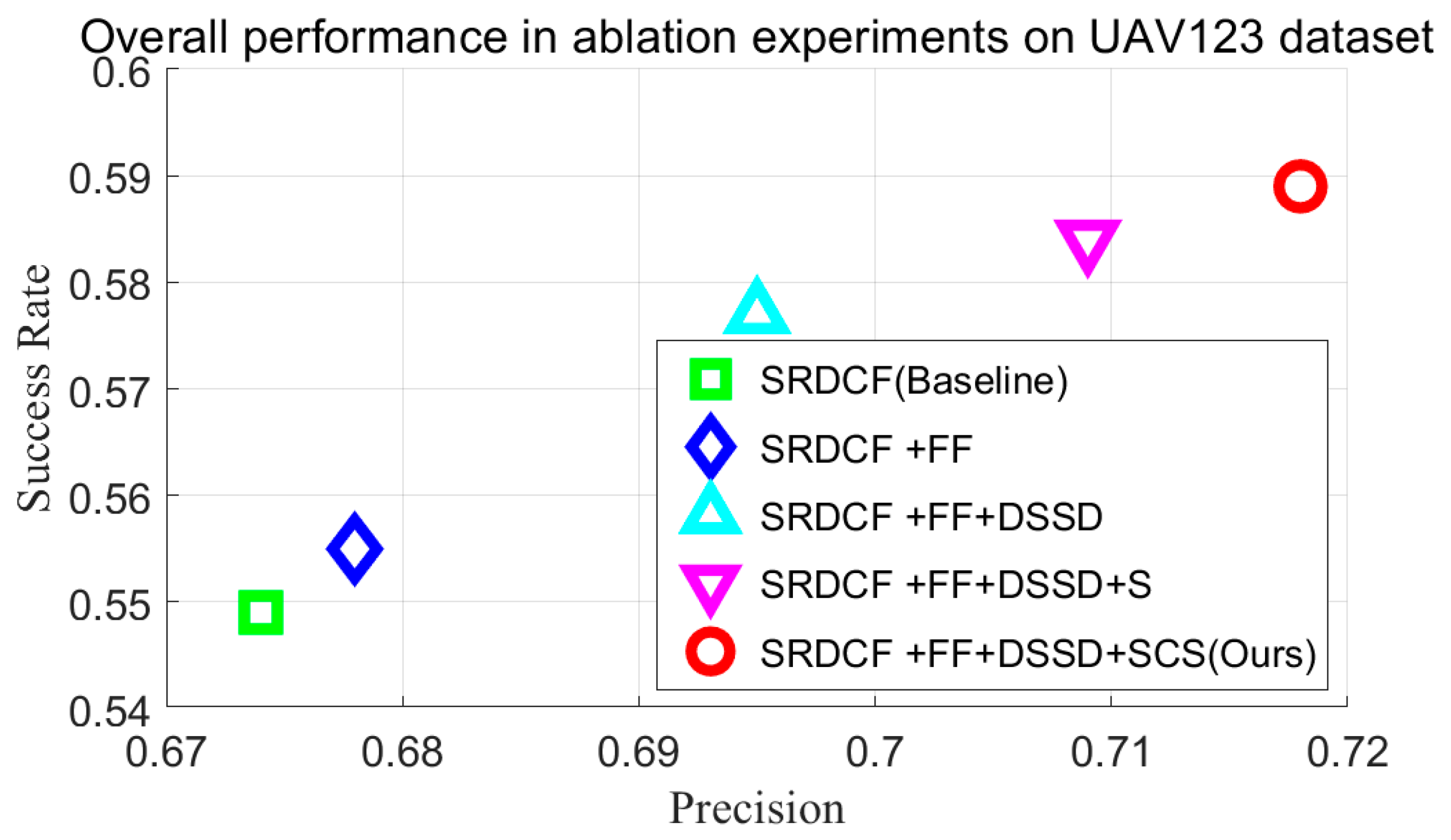
This paper proposed a robust UAV target tracking algorithm SDBCF based on saliency detection. As UAV target tracking is easily affected by background clutter, similar object interference, camera motion, occlusion, scale changes and other factors, improvement strategies for SRDCF were proposed, focusing on three aspects: feature fusion, model construction, and scale estimation. In terms of feature fusion, SDBCF fully exploits the spatial and temporal information of features, achieving the dynamic fusion of features in complex scenes. In terms of model construction, SDBCF integrates dynamic spatial regularization terms and second-order differential regularization terms into the DCF framework, improving the robustness of the filter in scenarios such as background clutter, similar object interference, and occlusion. In terms of scale estimation, SDBCF achieves adaptive response to changes in target aspect ratio and can continuously estimate changes in target scale, effectively improving the tracker’s ability to cope with scale changes. SDBCF utilizes significance detection methods to connect various modules together, fully leveraging the role of significance detection. Comparative experiments conducted on the UAV123, UAV20L, and DTB70 datasets showed that SDBCF had the best DP and AUC scores on all three datasets, with improvements of (4.1%, 5.0%), (9.9%, 15.4%), and (21.1%, 12.3%) compared to SRDCF, respectively. When facing similar background interference, background clutter, occlusion, scale variation, aspect ratio variation, camera motion, etc., the tracking performance of SDBCF is significantly better than other tracking methods, fully demonstrating the superiority of SDBCF.

Although the tracking performance of SDBCF has significantly improved, SDBCF only uses manual features and has a limited ability to represent targets, resulting in poor performance in, for example, low-resolution scenarios. Therefore, in the next step, we will consider introducing deep features into the feature fusion module to further improve the tracking performance of SDBCF without significantly affecting the tracking speed. At the same time, it was found during the experiment that SDBCF had poor robustness in scenarios such as complete occlusion and objects being out of view. This is because SDBCF did not design reliability detection modules and redetection modules, and therefore cannot respond to tracking failures in a timely manner. Therefore, we will also consider carrying out related work. In addition, the scale estimation strategy proposed by SDBCF is actually a universal scale estimation method for DCF trackers. Therefore, the next step will be to conduct relevant experiments to further investigate the performance of the scale estimation module on other trackers.

References

1. Zhang, J.; Zhang, X.; Huang, Z.; Cheng, X.; Feng, J.; Jiao, L. Bidirectional Multiple Object Tracking Based on Trajectory Criteria in Satellite Videos. IEEE Trans. Geosci. Remote Sens. 2023, 61, 1–14. [Google Scholar]
2. Siddharth, R.; Aghila, G. A Fog-Assisted Framework for Intelligent Video Preprocessing in Cloud-based Video Surveillance as a Service. IEEE Trans. Sustain. Comput. 2022, 7, 1. [Google Scholar]
3. Bu, Y.; Xie, L.; Gong, Y.; Wang, C.; Yang, L.; Liu, J.; Lu, S. RF-Dial: Rigid Motion Tracking and Touch Gesture Detection for Interaction via RFID Tags. IEEE Trans. Mob. Comput. 2022, 21, 1061–1080. [Google Scholar]
4. Stodola, P. Improvement in the model of cooperative aerial reconnaissance used in the tactical decision support system. J. Def. Model. Simul. 2017, 14, 483–492. [Google Scholar]
5. Mu, L.; Xie, G.; Yu, X.; Wang, B.; Zhang, Y. Robust Guidance for a Reusable Launch Vehicle in Terminal Phase. IEEE Trans. Aerosp. Electron. Syst. 2022, 58, 1996–2011. [Google Scholar] [CrossRef]
6. Li, Y.; Fu, C.; Ding, F.; Huang, Z.; Lu, G. AutoTrack: Towards High-Performance Visual Tracking for UAV with Automatic Spatio-Temporal Regularization. In Proceedings of the 2020 IEEE/CVF Conference on Computer Vision and Pattern Recognition (CVPR), Seattle, WA, USA, 13–19 June 2020. [Google Scholar]
7. Luo, W.; Biao, L.; Ruigang, F. Infrared Ground Multi-object Tracking Method Based on Improved ByteTrack Algorithm. Comput. Sci. 2023, 50, 176–183. [Google Scholar] [CrossRef]
8. Xie, Z.; Xu, Z.; Han, S.; Zhu, J.; Huang, X. Modulus Constrained Minimax Radar Code Design Against Target Interpulse Fluctuation. IEEE Trans. Veh. Technol. 2023, 72, 13671–13676. [Google Scholar]
9. Bolme, D.S.; Beveridge, J.R.; Draper, B.A.; Lui, Y.M. Visual object tracking using adaptive correlation filters. In Proceedings of the 2010 IEEE Computer Society Conference on Computer Vision and Pattern Recognition, San Francisco, CA, USA, 13–18 June 2010. [Google Scholar]
10. Henriques, J.F.; Caseiro, R.; Martins, P.; Batista, J. Exploiting the Circulant Structure of Tracking-by-detection with Kernels. In Proceedings of the European Conference on Computer Vision, Florence, Italy, 7–13 October 2012. [Google Scholar]
11. Henriques, J.F.; Caseiro, R.; Martins, P.; Batista, J. High-speed tracking with kernelized correlation filters. IEEE Trans. Pattern Anal. Mach. Intell. 2015, 37, 583–596. [Google Scholar]
12. Danelljan, M.; Shahbaz Khan, F.; Felsberg, M.; Van de Weijer, J. Adaptive Color Attributes for Real-Time Visual Tracking. In Proceedings of the 2014 IEEE Conference on Computer Vision and Pattern Recognition, Columbus, OH, USA, 23–28 June 2014. [Google Scholar]
13. Danelljan, M.; Robinson, A.; Khan, F.S.; Felsberg, M. Beyond correlation filters: Learning continuous convolution operators for visual tracking. In Proceedings of the 14th European Conference, Amsterdam, The Netherlands, 11–14 October 2016. [Google Scholar]
14. Wang, N.; Zhou, W.G.; Tian, Q.; Hong, R.C.; Wang, M.; Li, H.Q. Multi-Cue Correlation Filters for Robust Visual Tracking. In Proceedings of the 31st IEEE/CVF Conference on Computer Vision and Pattern Recognition (CVPR), Salt Lake City, UT, USA, 18–23 June 2018. [Google Scholar]
15. Danelljan, M.; Hager, G.; Khan, F.S.; Felsberg, M. Learning Spatially Regularized Correlation Filters for Visual Tracking. In Proceedings of the 2015 IEEE International Conference on Computer Vision (ICCV), Santiago, Chile, 7–13 December 2015. [Google Scholar]
16. Li, F.; Tian, C.; Zuo, W.; Zhang, L.; Yang, M.H. Learning Spatial-Temporal Regularized Correlation Filters for Visual Tracking. arXiv 2018, arXiv:1803.08679. [Google Scholar]
17. Li, Y.; Zhu, J. A Scale Adaptive Kernel Correlation Filter Tracker with Feature Integration. In Proceedings of the European Conference on Computer Vision, Zurich, Switzerland, 6–12 September 2014. [Google Scholar]
18. Danelljan, M.; Häger, G.; Khan, F.; Felsberg, M. Accurate Scale Estimation for Robust Visual Tracking. In Proceedings of the British Machine Vision Conference, Nottingham, UK, 1–5 September 2014. [Google Scholar]
19. Jiang, B.; Luo, R.; Mao, J.; Xiao, T.; Jiang, Y. Acquisition of localization confidence for accurate object detection. In Proceedings of the IEEE European Conference on Computer Vision, Munich, Germany, 8–14 September 2018; pp. 816–832. [Google Scholar]
20. Huang, Z.; Fu, C.; Li, Y.; Lin, F.; Lu, P. Learning aberrance repressed correlation filters for realtime uav tracking. In Proceedings of the 2019 IEEE/CVF International Conference on Computer Vision (ICCV), Seoul, Republic of Korea, 27 October–2 November 2019; p. 28912900. [Google Scholar]
21. Xing, W.; Zhang, H.; Wu, Y.; Li, Y.; Yuan, D. Redefined target sample-based background-aware correlation filters for object tracking. Appl. Intell. 2023, 53, 11120–11141. [Google Scholar] [CrossRef]
22. Zhang, J.; Yuan, T.; He, Y.; Wang, J. A background-aware correlation filter with adaptive saliency-aware regularization for visual tracking. Neural Comput. Appl. 2022, 34, 6359–6376. [Google Scholar] [CrossRef]
23. Ma, S.; Zhao, B.; Hou, Z.; Yu, W.; Pu, L.; Yang, X. SOCF: A correlation filter for real-time UAV tracking based on spatial disturbance suppression and object saliency-aware. Expert Syst. Appl. 2024, 238, 122131. [Google Scholar]
24. Yu, Y.-F.; Chen, Z.; Zhang, Y.; Zhang, C.; Ding, W. Learning Dynamic-Sensitivity Enhanced Correlation Filter with Adaptive Second-Order Difference Spatial Regularization for UAV Tracking. IEEE Trans. Intell. Transp. Syst. 2025, 1–20. [Google Scholar] [CrossRef]
25. Elayaperumal, D.; Joo, Y.H. Learning spatial variance-key surrounding-aware tracking via multi-expert deep feature fusion. Inf. Sci. Int. J. 2023, 629, 502–519. [Google Scholar]
26. Li, J.; Xue, C.; Luo, X.; Fu, Y.; Lin, B. Robust underwater object tracking with image enhancement and two-step feature compression. Complex Intell. Syst. 2025, 11, 154. [Google Scholar]
27. Zhang, Y.; Zheng, Y. Object Tracking in UAV Videos by Multi-Feature Correlation filters with Saliency Proposals. IEEE J. Sel. Top. Appl. Earth Obs. Remote Sens. 2023, 16, 5538–5548. [Google Scholar]
28. Zhang, J.; Feng, W.; Yuan, T.; Wang, J.; Sangaiah, A.K. SCSTCF: Spatial-Channel Selection and Temporal Regularized Correlation Filters for visual tracking. Appl. Soft Comput. 2022, 118, 108485. [Google Scholar]
29. Moorthy, S.; Joo, Y.H. Learning dynamic spatial-temporal regularized correlation filter tracking with response deviation suppression via multi-feature fusion. Neural Netw. 2023, 167, 360–379. [Google Scholar] [CrossRef]
30. Fu, C.; Xu, J.; Lin, F.; Guo, F.; Liu, T.; Zhang, Z. Object Saliency-Aware Dual Regularized Correlation Filter for Real-Time Aerial Tracking. IEEE Trans. Geosci. Remote Sens. 2020, 58, 8940–8951. [Google Scholar]
31. Yang, P.; Wang, Q.; Dou, J.; Dou, L. SDCS-CF: Saliency-driven localization and cascade scale estimation for visual tracking. J. Vis. Commun. Image Represent. 2024, 98, 104040. [Google Scholar]
32. Zhang, W. Saliency-enhanced background-aware correlation filters with dual temporal regularization for unmanned aerial vehicle tracking. J. Electron. Imaging 2024, 33, 023017. [Google Scholar] [CrossRef]
33. Arthanari, S.; Elayaperumal, D.; Joo, Y.H. Learning temporal regularized spatial-aware deep correlation filter tracking via adaptive channel selection. Neural Netw. 2025, 186, 107210. [Google Scholar] [CrossRef] [PubMed]
34. Wang, F.; Yin, S.; Mbelwa, J.T.; Sun, F. Context and saliency aware correlation filter for visual tracking. Multimedia Tools Appl. 2022, 81, 27879–27893. [Google Scholar] [CrossRef]
35. He, H.; Chen, Z.; Li, Z.; Liu, X.; Liu, H. Scale-Aware Tracking Method with Appearance Feature Filtering and Inter-Frame Continuity. Sensors 2023, 23, 7516. [Google Scholar] [CrossRef]
36. He, X.; Zhao, L.; Chen, C.Y.C. Variable scale learning for visual object tracking. J. Ambient Intell. Humaniz. Comput. 2023, 14, 3315–3330. [Google Scholar] [CrossRef]
37. Ma, H.; Lin, Z.; Acton, S.T. FAST: Fast and Accurate Scale Estimation for Tracking. IEEE Signal Process. Lett. 2020, 27, 161–165. [Google Scholar] [CrossRef]
38. Wu, Y.; Lim, J.; Yang, M. Object Tracking Benchmark. IEEE Trans. Pattern Anal. Mach. Intell. 2015, 37, 1834–1848. [Google Scholar] [CrossRef]
39. Chen, F.; Wang, X. Adaptive spatial-temporal regularization for correlation filters based visual object tracking. Symmetry 2021, 13, 1665. [Google Scholar] [CrossRef]
40. Hou, X.; Zhang, L. Saliency detection: A spectral residual approach. In Proceedings of the 2007 IEEE Conference on Computer Vision and Pattern Recognition, Minneapolis, MN, USA, 17–22 June 2007. [Google Scholar]
41. Nai, K.; Li, Z.; Wang, H. Dynamic feature fusion with spatial-temporal context for robust object tracking. Pattern Recognit. 2022, 130, 108775. [Google Scholar] [CrossRef]
42. Mueller, M.; Smith, N.; Ghanem, B. A benchmark and simulator for UAV tracking. In Proceedings of the 14th European Conference on Computer Vision, Amsterdam, The Netherlands, 11–14 October 2016; Springer: Amsterdam, The Netherlands, 2016; pp. 445–461. [Google Scholar]
43. Li, S.; Yeung, D.-Y. Visual Object Tracking for Unmanned Aerial Vehicles: A Benchmark and New Motion Models. In Proceedings of the Thirty-First AAAI Conference on Artificial Intelligence (AAAI-2017), San Francisco, CA, USA, 4–9 February 2017. [Google Scholar]
44. Wu, Y.; Lim, J.; Yang, M.-H. Online Object Tracking: A Benchmark. In Proceedings of the 2013 IEEE Computer Society Conference on Computer Vision and Pattern Recognition, Portland, OR, USA, 23–28 June 2013. [Google Scholar]
45. Galoogahi, H.K.; Fagg, A.; Lucey, S. Learning Background-Aware Correlation Filters for Visual Tracking. In Proceedings of the 2017 IEEE International Conference on Computer Vision (ICCV), Venice, Italy, 22–29 October 2017. [Google Scholar]
46. LuNežič, A.; Vojíř, T.; Zajc, L.Č.; Matas, J.; Kristan, M. Discriminative correlation filter tracker with channel and spatial reliability. Int. J. Comput. Vis. 2018, 126, 671–688. [Google Scholar] [CrossRef]
47. Bertinetto, L.; Valmadre, J.; Golodetz, S.; Miksik, O.; Torr, P.H. Staple: Complementary Learners for Real-Time Tracking. In Proceedings of the IEEE Conference on Computer Vision and Pattern Recognition (CVPR), Las Vegas, NV, USA, 27–30 June 2016. [Google Scholar]
48. Wen, J.; Chu, H.; Lai, Z.; Xu, T.; Shen, L. Enhanced robust spatial feature selection and correlation filter learning for UAV tracking. Neural Netw. 2023, 161, 39–54. [Google Scholar] [CrossRef]
Figure 1. Algorithm flowchart in this paper. The purple line in the figure represents the process related to position estimation, and the yellow line represents the process related to scale estimation.
Drones 09 00285 g001
Figure 2. Mask generation process. From (top) to (bottom): sample patch, saliency map, and mask. From (left) to (right): sequence boat1, building4, car16, and person5 in the UAV123 dataset. The red box represents the target area.
Drones 09 00285 g002
Figure 3. (a) Generated mask for search area; (b) search area response map; (c) target area response map; (d) non-target area response map.
Drones 09 00285 g003
Figure 4. OPE results of 10 algorithms on the UAV123, UAV20L, and DTB70 datasets.
Drones 09 00285 g004
Figure 5. Partial tracking results of the five trackers on different sequences. (a) Bird; (b) Group3; (c) Person7; (d) ChasingDrones; (e) Basketball.
Drones 09 00285 g005aDrones 09 00285 g005b
Figure 6. Partial tracking results of SDBCF on several sequences: (a) Boat3; (b) Car8; (c) wakeboard1; (d) Car16.
Drones 09 00285 g006aDrones 09 00285 g006b
Figure 7. Sensitivity analysis of the key parameters in SDBCF: (a) fusion weight coefficient analysis results; (b) differential regularization coefficient analysis results.
Drones 09 00285 g007
Figure 8. Overall performance of the five algorithms in ablation experiments on the UAV123.
Drones 09 00285 g008