Integrating Autonomous Vehicles and Drones for Last-Mile Delivery: A Routing Problem with Two Types of Drones and Multiple Visits

Abstract

With the growing demand for delivery services and the escalating labor costs, much effort has been made to achieve faster and cost-efficient delivery. A promising emerging strategy involves the integration of autonomous delivery vehicles or drones into the last-mile delivery. This study presents a fully automated last-mile delivery system that synergistically integrates autonomous vehicles and drones. We also introduce a novel variant of the vehicle routing problem with drones, referred to as the hybrid autonomous vehicle-drone routing problem (HAVDRP). In HAVDRP, we employ three delivery tools: autonomous vehicles, vehicle-carried drones, and independent drones. The aim is to fully leverage the advantages of autonomous vehicles and drones to provide customers with more efficient last-mile delivery services. An improved adaptive large neighborhood search algorithm is developed to address this problem. The algorithm incorporates a tabu list and an adaptive mechanism specifically designed for the HAVDRP, thereby augmenting the search efficiency. Computational experiments are conducted to evaluate the efficiency of the designed algorithm. Additionally, sensitivity analyses are conducted to explore the influences of some key parameters on the total time, which includes the cumulative working time of autonomous vehicles and drones. Based on the results of sensitivity analyses, we propose some management recommendations for the fully automated last-mile delivery system utilizing autonomous vehicles and drones.

1. Introduction

In recent years, the rapid development of the internet has fueled the growth of e-commerce and created significant opportunities for logistics. In conjunction with advancements in logistics infrastructure, the express delivery industry in China has witnessed substantial growth over the past decade. According to the State Post Bureau of The People’s Republic of China, the volume of express delivery in China reached 63.5 billion pieces in 2019, generating operating revenues of 749.8 billion CNY. By 2024, the volume had increased by 176% to 175.1 billion pieces compared to 2019, while the operating revenue reached 1403.4 billion CNY, reflecting a growth of 87% compared to 2019. However, the continuous growth in the volume of express delivery has rendered traditional manual operations inadequate to meet the escalating demand. Moreover, escalating labor costs have emerged as a bottleneck impeding the progress of the express delivery industry.

The use of drones has opened up new possibilities for last-mile delivery. Since 2013, several prominent companies, such as Amazon, UPS, and FedEx, have been conducting experiments in drone delivery for the last mile [1]. In 2021, Walmart piloted drone delivery to residential properties and planned further expansion. In China, by 2022, Meituan successfully implemented drone delivery in Shenzhen, achieving large-scale promotion, serving nearly 20,000 households, and completing over 120,000 orders. The EU drone regulations were established by the EU Aviation Safety Agency (EASA) and have been in effect since 1 January 2021 [2]. Simultaneously, the Chinese government has enacted the updated drone regulations, which came into effect on 1 January 2024. The Civil Aviation Administration of China (CAAC) has issued licenses to selected logistics companies for the operation of delivery drones [3]. It is expected that drone-based delivery will become more prevalent in the coming years. Drones offer advantages such as high flexibility and speed, yet their capacity and battery life are limited [4]. In contrast, trucks are characterized by slower speeds, larger capacities, and longer travel distances. Many scholars have attempted to combine trucks with drones for delivery and have conducted extensive research on the truck-drone routing problem (TDRP), as detailed in Section 2.2.

On the other hand, the rapid development of autonomous driving technology in recent years has also opened up new prospects for last-mile delivery. In 2016, several universities in the United States conducted trials of autonomous delivery vehicles (ADVs) applications on their campuses, encompassing delivery services such as mail, express, fresh food, and catering. During the COVID-19 pandemic, ADVs from companies such as JD.com and Neolix played a crucial role in ensuring the continuity of the supply chain through contactless delivery. In September 2023, Meituan’s ADVs initiated delivery services in Beijing’s Shunyi District at a maximum speed of 45 km/h, signifying the transition of ADVs from “pilot testing” to “large-scale application”.

In contrast to existing TDRP studies, our research introduces a fully automated last-mile delivery system that integrates ADVs and drones synergistically. Due to the remarkable advances in autonomous driving technology, the emergence of innovative services that leverage this technology is anticipated, such as autonomous taxis and ADVs. Considering the technology advancements and the pressing needs of last-mile delivery, this paper introduces a novel variant of the vehicle routing problem with drones for the fully automated last-mile delivery system, referred to as the Hybrid Autonomous Vehicle-Drone Routing Problem (HAVDRP). To the best of our knowledge, our research is the pioneering attempt to explore combined delivery using ADVs and drones.

Compared to traditional TDRP, HAVDRP has some differences and presents new challenges. First, unlike most existing TDRP, in our HAVDRP, drones require recharging on ADVs rather than battery swapping. Both autonomous vehicles and drones are battery-powered, so it is more convenient for ADVs to assist in recharging, as they can be charged at the depot. However, the dynamic battery status of the vehicle-carried drones (VDs) will be a significant challenge in modeling, which has been less addressed in existing TDRP research. Second, in the HAVDRP, we employ VDs to serve multiple customers in a single flight. While the battery life of the VDs is dynamic. Therefore, the model must consider more rigorous and complex constraints for the endurance time of VDs. Third, in the HAVDRP, autonomous vehicles are mixed with multiple VDs and multiple independent drones (IDs) for delivery. The complexity of task allocation and route optimization between the autonomous vehicles and drones is further amplified. Therefore, an effective algorithm must be taken into consideration to solve the problem.

Considering the characteristics of the HAVDRP, we formulate this problem as a mixed integer programming (MIP) and validate its correctness through small-sized problems solved by Gurobi solver. To address the larger-sized problems, we have designed an improved adaptive large neighborhood search (IALNS) algorithm, which can solve the large-sized problems within a reasonable time. The main contributions of this paper are as follows:

(1)

A novel variant of the vehicle routing problem with drones (VRPD) is proposed for the fully automated last-mile delivery system, termed the hybrid autonomous vehicle-drone routing problem (HAVDRP). This new variant addresses the integration of autonomous ground and aerial delivery systems, offering a potential solution to the evolving unmanned last-mile delivery;

(2)

A mixed integer programming (MIP) model is established to represent the HAVDRP. Within the MIP model, we incorporate the dynamic battery levels of the vehicle-carried drones and the endurance time constraints under these dynamic battery levels. These aspects have been less explored in existing research;

(3)

An IALNS algorithm is specifically designed to solve the HAVDRP. Accounting for the complexity of the HAVDRP, several improvements are incorporated into the basic ALNS algorithm, including targeted optimization operators tailored for the HAVDRP, improved adaptive mechanism with a tabu list, and a reinitialization procedure. The effectiveness of the IALNS algorithm is validated through computational experiments;

(4)

Sensitivity analyses on key parameters in the HAVDRP are conducted, including the number of vehicle-carried drones, drone speed, and drone capacity. Based on the findings, we provide management recommendations for the application of ADVs and drones in last-mile delivery.

This paper is organized as follows: Section 2 reviews relevant research on the AVRP and VRPD. Section 3 presents the problem scenario and establishes a novel mixed integer programming model for the HAVDRP. In Section 4, a detailed description of the designed algorithm to solve the HAVDRP is provided. Section 5 employs the algorithm to solve the HAVDRP in computational experiments and conducts sensitivity analyses on key parameters. Finally, Section 6 summarizes the research conclusions and proposes future research directions.

2. Related Work

This paper studies the hybrid delivery problem integrating ADVs and drones, which is concerned with autonomous vehicle routing problem (AVRP) while also addressing the truck-drone routing problem (TDRP). Therefore, relevant studies on AVRP are reviewed first, followed by a survey of the literature pertaining to TDRP.

2.1. Autonomous Vehicle Routing Problem

The autonomous delivery vehicle (ADV) is an emerging technological innovation with the potential to revolutionize conventional logistic delivery models [5]. Several studies have been conducted to investigate the public acceptance of ADVs. According to the survey conducted by Kapser and Abdelrahman [6] among the German public, price emerged as the primary determinant influencing willingness to accept ADVs, followed by considerations of social impact and convenience. AlKheder et al. [7] conducted a study during the COVID-19 pandemic in Kuwait to examine customer perceptions and acceptance of ADVs. The findings revealed that male participants placed greater emphasis on perceived risks, while female participants expressed higher concerns regarding the reliability of on-time delivery. Figliozzi [8] explored the potential of unmanned aerial vehicles (UAVs), sidewalk automated delivery robots (SADRs), and road automated delivery robots (RADRs) in mitigating carbon emissions. They found that RADRs can significantly contribute to carbon emission reduction in medium-sized service areas. Lemardelé et al. [9] investigated the applicability of drones and ground automated delivery devices (GADDs) in last-mile logistics. The research highlighted that the integration of GADDs and the urban consolidation centers (UCC) strategy is a more economically viable approach in high-density and small-area service areas. These studies provide valuable insights into the significance and feasibility of ADV applications, thereby establishing a robust foundation for their practical implementation.

Numerous scholars have conducted research on the practical application of ADVs. Scherr et al., Liu et al., and Farahani et al. [10,11,12] examined the formation of mixed fleets consisting of ADVs and conventional vehicles for logistics delivery. Scherr et al. [10] proposed a model wherein autonomous vehicles (AVs) operate independently in specific areas and are guided by manually driven vehicles in other areas. Liu et al. [11] investigated the two-echelon vehicle routing problem with a heterogeneous fleet, comprising conventional trucks and ADVs for efficient delivery. Farahani et al. [12] investigated the mixed fleet delivery problem, taking into account customer time windows, ADV charging at stations, and infrastructure limitations for ADVs on specific roads. The findings of their research demonstrated that incorporating ADVs into logistics operations can yield a significant reduction in costs. Ulmer and Streng [13] focused on the same-day delivery problem using AVs and pick-up points, where customers can place dynamic orders within a day and select nearby pick-up points as delivery locations. Yu [14] explored an autonomous vehicle logistic system that facilitates the autonomous charging of AVs at distributed generations or depots to meet customer demands within specified time windows.

Furthermore, some scholars have investigated more specific constraints in the context of AVRPs. Nasri et al. [15] aimed at optimizing routes and speeds for autonomous trucks under uncertain traffic conditions, with the objective of minimizing fuel consumption, emissions, and costs. Bray and Cebon [16] examined the selection of vehicle size in the multi-destination routing problem for AVs, suggesting that employing smaller AVs can result in additional cost savings in specific scenarios, extending beyond driver expenses. Li et al. [17] explored the dynamic vehicle routing problem for ADVs, taking into account factors such as road conditions, traffic congestion, and weather conditions. Moradi et al. [18] focused on the AVRP for last-mile delivery in urban areas, incorporating a constraint to ensure that the walking distances for customers do not exceed a predetermined threshold. Wang et al. [19] investigated the spatiotemporal routing problem for a fleet of ADVs, considering the stochastic nature of customer service and arrival time.

2.2. Truck-Drone Routing Problem

In recent years, there has been a growing interest in the use of UAVs, commonly known as drones, which are considered as an innovative solution for last-mile delivery [20]. Silva et al. [21] studied the acceptance of urban air mobility (UAM) for e-commerce delivery in different regions of Europe. The findings indicate that the public generally holds a positive attitude towards the application of UAM. However, the limitations of drones, such as their restricted payload capacity and flight endurance, have motivated researchers to investigate the integration of UAVs with trucks, which has given rise to a novel research domain known as the truck-drone routing problem (TDRP). To review the related works, we classify the TDRPs into two categories based on different coordination approaches: the truck-drone collaborative delivery problem and the truck-drone parallel delivery problem.

2.2.1. Truck-Drone Collaborative Delivery Problem

The truck-drone collaborative delivery problem has been extensively investigated through a substantial amount of research [22,23]. In this section, we review the relevant works under two subdivisions: the traveling salesman problem with drones (TSP-D) and the vehicle routing problem with drones (VRP-D).

(1)

TSP-D

The first research on TSP-D, specifically focusing on a single drone and a single truck (TSP-1D), was conducted by Murray and Chu [24], who assumed the existence of a single depot and multiple customers to be serviced either by the truck or the drone. The objective was to minimize delivery time. Carlsson and Song [25] argued that TSP-1D should enable the truck and the drone to rendezvous at any arbitrary location, rather than being limited to only the depot or customer sites. Agatz et al. [26] developed a mathematical model for TSP-1D and proposed a heuristic algorithm that combines local search and dynamic programming techniques to efficiently solve large-sized instances. Dell’Amico et al. [27] and Boccia et al. [28] used exact algorithms to address the TSP-1D problem.

Recently, many researchers have introduced more detailed considerations regarding the scenarios and constraints of TSP-1D. Amorosi et al. [29] explored the mothership and drone routing problem with graphs (MDRPG), which involves a delivery route graph for the drone. El-Adle et al. [30] allowed the drone to be launched and received at any node, which means it can either take off and land at different or the same nodes. Jeong et al., Cho et al., and Tamke and Buscher [31,32,33] focused on the energy consumption of trucks and the drone in TSP-1D. Jeong et al. [31] investigated the impact of payload weight on drone energy consumption, while Cho et al. [32] integrated terrain, road gradient, and payload factors into their energy consumption model for the electric truck and the drone. Additionally, Tamke and Buscher [33] examined the influence of drone speed on both energy consumption and delivery range.

Following the research on TSP-1D, scholars further expanded their investigations to the TSP-D with one truck carrying multiple drones (TSP-mD). Tu et al. [34] employed two heuristic algorithms to solve the TSP-mD and evaluated their performance on different-sized instances. The results indicated that the adaptive large neighborhood search algorithm (ALNS) outperformed the greedy randomized adaptive search procedure (GRASP), as it provided lower-cost solutions. Karak and Abdelghany [35] expanded the TSP-mD by considering the hybrid vehicle-drone routing problem (HVDRP), which integrates both vehicles and UAVs for efficient pickup and delivery services. Murray and Raj [36] examined a last-mile delivery system, where a heterogeneous fleet of UAVs and trucks collaboratively served customers. They considered the endurance of drones in relation to their payload and speed. Building on this research, Raj and Murray [37] further considered the drone’s speed as a decision variable with the aim of minimizing the total time.

Moreover, researchers such as Leon-Blanco et al. [38] and Deng et al. [39] have explored the feasibility of utilizing the UAV for multi-deliveries within a single flight. Other scholars have examined different coordination approaches between trucks and UAVs. For example, Moshref-Javadi et al. [40] investigated a scenario with a truck carrying multiple UAVs, synchronizing them at three different levels. Tiniç et al. [41] enabled the launch and reception of UAVs at any customer nodes, regardless of whether they are identical or distinct. Betti Sorbelli et al. [42] considered conflicts between trucks and multiple UAVs. These studies significantly contribute to the advancement and enrichment of TDRP.

(2)

VRP-D

In contrast to TSP-D, VRP-D requires the coordination of multiple vehicles and drones for delivery, which adds much more complexity to the problem. Primarily, we review the VRP-D problem where each vehicle collaborates with one drone (VRP-1D). Sacramento et al. [43] proposed a mathematical model for the VRP-1D and designed the ALNS algorithm to solve it. In their study, the drone could take off and land at customer nodes along the truck route, enabling simultaneous delivery by both the drone and the truck. Chiang et al. [44] incorporated energy consumption, carbon emissions, and transportation costs into the VRP-1D, and developed an improved genetic algorithm to effectively solve it. Wang et al. [45] investigated a hybrid truck-drone delivery problem, wherein trucks and two types of drones (independent drones and truck-carried drones) were employed. The drones can serve multiple customers within their capacity and flight range, which is similar to the problem in our study. Lei et al. [46] employed a novel dynamical artificial bee colony (DABC) algorithm to solve the problem proposed by Sacramento et al. [43]. Kuo et al. [47] extended the model developed by Sacramento et al. [43] and proposed an improved variable neighborhood search (VNS) to solve it.

Some scholars have further extended VRP-1D in different ways. Huang et al. [48] introduced a threshold of the waiting time of trucks at a customer location for drone receiving. Wei et al. studied the time-dependent VRP-1D with vehicle-restricted zones and no-fly zones [49]. Zang et al. [50] considered VRP-1D with parking points, which exclusively serve as launch and retrieval locations for drones. Gu et al. [51] studied the VRP-1D with multiple visits, wherein a drone could visit multiple customers in a single flight while adhering to its limited endurance and capacity constraints. Scholars have also considered the VRP-1D with different types of vehicles. Imran et al. [52] examined the fully automated last-mile delivery problem using AVs and drones, referred to as the autonomous vehicle routing problem with drones (A-VRPD). Ren et al. [53] investigated the last-mile delivery problem using electric vehicles, drones and battery-swap vehicles.

Building upon VRP-1D, scholars have extended their research to the VRP-mD problem, wherein each vehicle collaborates with multiple drones. Wang et al. [54] studied VRP-mD, wherein each drone could carry only one package. They primarily used worst-case analysis to compare the performance of different solutions, providing a foundation and inspiration for further research in VRPD. Schermer et al. [55] investigated VRP-mD with cyclic drone operations, specifically focusing on takeoff and landing at the same location, and developed a mixed integer linear programming (MILP) model with the objective of minimizing the completion time. They proposed a heuristic algorithm to solve it. Wang and Sheu and Rave et al. [56,57] both studied VRP-mD with transfer stations. In Wang and Sheu [56], drones were restricted to launching and receiving exclusively at the depot or transfer stations, rather than at customer locations. In Rave et al. [57], transfer stations acted as micro-depots where drones and trucks could depart from and visit. The transfer stations had fixed usage costs and required delivery by trucks. Kitjacharoenchai et al. [58] addressed the two-echelon VRP with multiple drones (2E-VRP-mD). They designed the drone-truck route construction (DTRC) heuristic and the large neighborhood search (LNS) algorithm to efficiently solve the problem.

Moreover, in the 2E-VRP-mD proposed by Zhou et al. [59], the number of drones each truck could carry was optimized as a decision variable. Lin et al. [60] tackled the discrete optimization problem in the truck-drone collaborative transport system for the efficient distribution of medical resources, emphasizing urgent delivery to customers within specified time limits. Gao et al. [3] investigated VRP-mD and considered the operating time and costs of trucks and drones, which are influenced by factors such as battery capacity, demand, and flight distance. They designed a column generation-based heuristic to solve the problem. Luo et al., Jiang et al., and Faiz et al. [61,62,63] researched the VRP-mD with drone multi-visit. Luo et al. [61] allow the drone to serve another customer requiring pick-up service after completing a delivery service. Jiang et al. [62] studied a multi-visit flexible-docking vehicle routing problem with drones for simultaneous pickup and delivery services. The problem also allows drones to perform flexible docking to the same or different trucks. Faiz et al. [63] proposed a novel two-echelon vehicle routing framework during post-disaster humanitarian operations. The framework employs two types of drones: hotspot drones capable of capturing demands and their locations, and delivery drones used to satisfy these demands. They designed a decomposition algorithm inspired by column generation to address the problem.

2.2.2. Truck-Drone Parallel Delivery Problem

The truck-drone parallel delivery problem (PDSTSP) was initially investigated by Murray and Chu [24], who aimed to minimize the delivery time by scheduling truck and drone routes. Subsequent studies conducted by Mbiadou Saleu et al., Dell’Amico et al., and Lei and Chen [64,65,66] proposed more efficient heuristic algorithms to solve the PDSTSP. Li et al. [67] extended the PDSTSP by considering multiple depots, while Schermer et al. [68] addressed the issue of drone battery life by proposing the PDSTSP with drone stations.

Furthermore, researchers have explored the parallel drone scheduling vehicle routing problem (PDSVRP), which involves multiple vehicles. Ham and Montemanni and Dell’Amico [69,70] used the constraint programming (CP) model to solve this problem. Ham [69] considered scenarios where customers had multiple demands with varying delivery time windows and priorities, while Montemanni and Dell’Amico [70] proposed two variants of PDSVRP: minimum time PDSVRP and minimum cost PDSVRP. Ulmer and Thomas and Ramos and Vigo [71,72] examined the dynamic PDSVRP for same-day deliveries. The collaboration between drones and trucks has been found to yield significant reductions in both delivery time and costs, as emphasized by both studies. Their difference lies in that Ramos and Vigo incorporated the time window into their research. Nguyen et al. [73] investigated cost-minimizing PDSVRP and proposed an effective metaheuristic to solve it. Mbiadou Saleu et al. [74] focused on minimizing the completion time in PDSVRP by employing a hybrid metaheuristic algorithm. They provided some suggestions for the truck-drone collaborative delivery system according to their research.

Table 1. The key features of VRP-D research.

Paper	Driver	#V 1	#D 2	#MV 3	Hybrid Delivery	Objective	Algorithm
Sacramento et al. [43]	yes	m	1	no	no	cost	ALNS
Chiang et al. [44]	yes	m	1	no	no	emissions cost	GA
Wang et al. [45]	yes	m	1	yes	yes	time	HTDD
Lei et al. [46]	yes	m	1	no	no	cost	DABC
Kuo et al. [47]	yes	m	1	no	no	cost	VNS
Huang et al. [48]	yes	m	1	no	no	cost	ACO
Zang et al. [50]	yes	m	1	no	no	cost	BH, TH
Gu et al. [51]	yes	m	1	yes	no	cost	ILS-VND
Imran et al. [52]	no	m	1	yes	no	cost	Greedy
Ren et al. [53]	yes	m	1	yes	no	cost	LNS-QL
Schermer et al. [55]	yes	m	n	no	no	time	Matheuristic
Wang and Sheu [56]	yes	m	n	yes	no	cost	B&C
Kitjacharoenchai et al. [58]	yes	m	n	yes	no	time	DTRC and LNS
Lin et al. [60]	yes	m	n	no	no	time	HA
Rave et al. [57]	yes	m	n	no	yes	cost	ALNS
Zhou et al. [59]	yes	m	n	no	no	time	B&P
Gao et al. [3]	yes	m	n	no	no	cost	CG
Luo et al. [61]	yes	m	n	yes	no	cost and waiting time	ODEA-ARA
Jiang et al. [62]	yes	m	n	yes	no	cost	ALNS
Faiz et al. [63]	yes	m	n	yes	no	cost	DA and CG
This paper	no	m	n	yes	yes	time	IALNS

¹ #V: Number of vehicles. ² #D: Number of drones carried by each vehicle. ³ #MV: Drone multi-visit.

provides a summary of key features in VRP-D research since 2019, as mentioned in Section 2.2.1. The table indicates that the majority of research still involves driver-operated vehicles, with only Imran et al. [52] exploring the use of AVs to support drone deliveries. In contrast, our study introduces ADVs that can both support drone and independent deliveries. Furthermore, unlike previous studies in Table 1, we consider scenarios where vehicle-carried drones can be recharged on ADVs and a hybrid delivery method involving collaboration between two types of drones and ADVs. These areas are complex and have been less extensively researched.

3. Problem Statement and Mathematical Model

3.1. Problem Description

In this paper, we aim to schedule the last-mile delivery routes for ADVs and drones through the HAVDRP. In the HAVDRP, a fleet of autonomous delivery vehicles (ADVs), ADV-carried drones (VDs), and independent drones (IDs) collaborate to provide delivery services to a set of customers. The ADVs carry a certain number of VDs and depart from a depot, serving a group of customers before returning to the depot. Each ADV is dispatched only once. The VDs can be launched from the ADV at the depot or customer nodes to serve a group of customers before returning to the same ADV, and can be dispatched multiple times within their battery life range. On the other hand, the IDs depart from the depot, provide services to a group of customers, and then return to the depot. They can also be dispatched multiple times to serve different customers.

Figure 1 illustrates an example of HAVDRP, where two ADVs and five drones serve 18 customers. An independent drone, D1, completes deliveries for five customers through three separate flights. The rest of the customers are served by the ADVs equipped with two VDs each. During the delivery process, the ID can only be launched and received at the depot, while the VDs can be launched and received both at the depot and different customer nodes along the ADV route. Both the ADVs and drones have limitations on battery life and maximum payload capacity. Additionally, IDs have a maximum working time constraint, which limits the number of flights they can make to serve customers.

Before formulating the mathematical model for HAVDRP, the important assumptions are summarized as follows:

(1)

IDs can swap their batteries at the depot, and VDs can recharge their batteries on the ADVs;

(2)

ADVs travel on ground roads, necessitating the use of the Manhattan distance to measure distances between nodes. Conversely, drones navigate through airspace, employing the Euclidean distance as their travel distance;

(3)

Upon arrival at a receiving node, both ADVs and drones are required to adhere to a protocol that the first-arriving vehicle waits for the other, with the assumption that neither ADVs nor drones consume energy while waiting at customer nodes;

(4)

The launch and receive time for drones is short (typically 30~60 s) and has negligible impact on the routes of the ADVs and drones [75]. Therefore, it is negligible;

(5)

IDs are permitted to depart from the depot for cyclic deliveries, whereas VDs are prohibited from undertaking the same operations;

(6)

The charging rate of VDs represents the additional endurance time gained per minute of charging. For instance, a charging rate of 1.5 means that charging a VD for 1 min extends its endurance by 1.5 min.

3.2. Notations and Mathematical Formulation

Based on the problem’s description, we establish the mathematical model for the HAVDRP problem. The composition of the mathematical model is shown in Figure 2, and the notations used are listed in

Table 2. The notations used in mathematical model.

Index Sets	Description
$V^C$	Set for customers
$V=\{0, c+1\}\cup V_C$	Set for all nodes including start node (depot), customer nodes and end node (depot)
$V^S=\left\{0\right\}\cup V^C$	Set for start nodes of arcs
$V^E=V^C\cup \left\{c+1\right\}$	Set for end nodes of arcs
$K^T$	Set for ADVs
$K^D$	Set for all drones including IDs and VDs
$K_0^D$	Set for IDs
$K_k^D$	Set for VDs carried by ADV $k(k\in K^T)$
$R_u^D$	Set for flights of drone $u(u\in K^D)$
Parameters
$D_i$	Demand from customer $i(i\in V^C)$
$Q^T$/$Q^D$	Maximum payload capacity of ADVs/drones
$B^T$/$B^D$	Maximum endurance time of ADVs/drones
$B^C$	Time for battery swap of IDs
$\mu$	The charging rate of drones on ADVs
${\Gamma }_{i,j}$/${\tau }_{i,j}$	Travel time of ADVs/drones from node $i$ to node $j$
$M$	A sufficiently large positive number
Decision Variables
$v_{i,k}^T$	Binary variable, 1 if ADV$k$ serves customer$i$, 0 otherwise
$v_{i,p,u}^D$	Binary variable, 1 if drone$u$ serves customer$i$ in $p$th flight, 0 otherwise
$x_{i,j,k}^T$	Binary variable, 1 if ADV$k$ travels arc $(i,j)$, 0 otherwise
$x_{i,j,p,u}^D$	Binary variable, 1 if drone $u$ travels arc $(i,j)$ in $p$th flight, 0 otherwise
$y_{i,p,u}^L$/$y_{i,p,u}^R$	Binary variable, 1 if drone $u$ is launched/received at node $i$ in $p$th flight, 0 otherwise
Other Variables
$T_{i,k}^T$	Continuous variable, the cumulative working time for ADV $k$ to arrive at node $i$
$T_{i,u}^D$	Continuous variable, the cumulative working time for VD $u$ to arrive at node $i$
$T_{i,p,u}^{D^{\prime }}$	Continuous variable, the cumulative working time for ID $u$ to arrive at node $i$ in $p$th flight
$T_{p,u}^L$	Continuous variable, the cumulative working time when drone $u$ is launched in $p$th flight.
$T_{p,u}^R$	Continuous variable, the cumulative working time when drone $u$ is received in $p$th flight.
$E_{i,u}^D$	Continuous variable, the endurance time for the battery of VD $u$ at node $i$
$r_u$	Integer variable, the last flight for VD $u(r_u\in R_u^D)$
$Z_{p,u}^D$	Binary variable, 1 if drone $u$ serves at least one customer in $p$th flight, 0 otherwise
$Z_{p,u}^{D^{\prime }}$	Binary variable, 1 if the ID $u$ serves at least one customer in $p$th flight, 0 otherwise

. It is important to note that the model incorporates time synchronization constraints between ADVs and multiple VDs in the time constraints. Additionally, the endurance constraints in the model account for the charging constraints of VDs when they are aboard ADVs. These constraints increase the complexity of the mathematical model while making it more applicable to real-life scenarios.

3.2.1. Objective Function

Inspired by the research of Kitjacharoenchai et al. [58] and Zhou et al. [59], our model’s objective is to minimize the total duration of all routes, including those of ADVs and IDs. It aims to improve the delivery efficiency.

$$\min Z_1=\sum _{k\in K^T}{T}_{c+1,k}^T+\sum _{u\in K_0^D}{T}_{c+1,r_u,u}^{D^{\prime }}$$

(1)

3.2.2. Customer Service Constraint

Constraint (2) specifies that each customer node can be serviced exactly once by either an ADV or a drone.

$$\sum _{k\in K^T}{v}_{i,k}^T+\sum _{u\in K^D}\sum _{p\in R_u^D}{v}_{i,p,u}^D=1, \forall i\in V^C$$

(2)

3.2.3. Routing Constraints

The HAVDRP problem incorporates two types of routes: the ADV routes and the drone routes, which are characterized by distinct features. Therefore, the routing constraints can also be divided into routing constraints of ADVs and routing constraints of drones.

(1)

Routing constraints of ADVs

Constraint (3) requires that ADVs start and end their routes at the depot. Constraint (4) signifies that the ADVs must visit and leave the customers served by them.

$$\sum _{j\in V^E}{x}_{0,j,k}^T=\sum _{i\in V^S}{x}_{i,c+1,k}^T\le 1,\forall k\in K^T$$

(3)

$$\sum _{i\in V^S}{x}_{i,j,k}^T=\sum _{h\in V^E}{x}_{j,h,k}^T=v_{j,k}^T, \forall k\in K^T, \forall j\in V^C$$

(4)

(2)

Routing constraints of Drones

Constraint (5) ensures that each customer served by drones must be in a specific flight. Constraint (6) requires that each flight of an ID must start and end at the depot. Constraint (7) represents the flow conservation of ID routes.

$$\sum _{i\in V^C}{v}_{i,p,u}^D\le M{Z}_{p,u}^D,\forall u\in K^D,\forall p\in R_u^D$$

(5)

$$\sum _{j\in V^E}{x}_{0,j,p,u}^D=\sum _{i\in V^S}{x}_{i,c+1,p,u}^D=1, \forall u\in K_0^D,\forall p\in R_u^D$$

(6)

$$\sum _{i\in V^S}{x}_{i,j,p,u}^D=\sum _{h\in V^E}{x}_{j,h,p,u}^D=v_{j,p,u}^D, \forall u\in K_0^D, \forall p\in R_u^D,\forall j\in V^C$$

(7)

Constraints (8)–(20) represent the flow conservation of VD routes. Constraints (8) and (9) guarantee that the launch and receive nodes of VDs must be customer nodes served by an ADV. Constraints (10) and (11) stipulate that each flight of the VDs must have only one launch node and only one receive node. Constraint (12) represents the flow conservation for each flight of the VDs, including the nodes served by them, the launch nodes and the receive nodes. Constraints (13) and (14) ensure that the subroute of VDs in each flight must start at launch nodes and end at receive nodes. Constraint (15) specifies that the route of VDs cannot start and end at the depot directly. Constraints (16) and (10) ensure that there is both a launch node and a receive node when the VD serves a customer. In constraint (16), the notation $\forall u\in K_k^D$ represents the drones carried by ADV $k$, while the inclusion of $\forall k\in K^T$ indicates that this constraint must be satisfied by all VDs across the entire delivery fleet. Subsequent constraints using $\forall u\in K_k^D$ and $\forall k\in K^T$ consistently adhere to this semantic interpretation. Constraints (17) and (18) limit that the same VD can visit and leave a customer node no more than once, while constraints (19) and (20) enforce that the same VD can be launched or received at the same node only once.

$$\sum _{u\in K_k^D}\sum _{p\in R_u^D}{y}_{i,p,u}^L\le M{v}_{i,k}^T,\forall k\in K^T,\forall i\in V^C$$

(8)

$$\sum _{u\in K_k^D}\sum _{p\in R_u^D}{y}_{i,p,u}^R\le M{v}_{i,k}^T,\forall k\in K^T,\forall i\in V^C$$

(9)

$$\sum _{i\in V^S}{y}_{i,p,u}^L=\sum _{i\in V^E}{y}_{i,p,u}^R,\forall u\in K_k^D,\forall k\in K^T,\forall p\in R_u^D$$

(10)

$$\sum _{i\in V^S}{y}_{i,p,u}^L\le 1,\forall u\in K_k^D,\forall k\in K^T,\forall p\in R_u^D$$

(11)

$$\begin{gathered} \sum _{i\in V^S}{x}_{i,j,p,u}^D+\sum _{h\in V^E}{x}_{j,h,p,u}^D=2v_{j,p,u}^D+y_{j,p,u}^L+y_{j,p,u}^R, \\ \forall u\in K_k^D,\forall k\in K^T,\forall p\in R_u^D,\forall j\in V^C \end{gathered}$$

(12)

$$y_{j,p,u}^L\le \sum _{h\in V^E}{x}_{j,h,p,u}^D,\forall u\in K_k^D,\forall k\in K^T,\forall p\in R_u^D,\forall j\in V^S$$

(13)

$$y_{j,p,u}^R\le \sum _{i\in V^S}{x}_{i,j,p,u}^D,\forall u\in K_k^D,\forall k\in K^T,\forall p\in R_u^D,\forall j\in V^E$$

(14)

$$y_{0,p,u}^L+y_{c+1,p,u}^R\le 1,\forall u\in K_k^D,\forall k\in K^T,\forall p\in R_u^D$$

(15)

$$\sum _{i\in V^C}{v}_{i,p,u}^D\le M\sum _{i\in V^S}{y}_{i,p,u}^L,\forall u\in K_k^D,\forall k\in K^T,\forall p\in R_u^D$$

(16)

$$\sum _{p\in R_u^D}\sum _{i\in V^S}{x}_{i,j,p,u}^D\le 1,\forall u\in K_k^D,\forall k\in K^T,\forall j\in V^E$$

(17)

$$\sum _{p\in R_u^D}\sum _{h\in V^E}{x}_{j,h,p,u}^D\le 1,\forall u\in K_k^D,\forall k\in K^T,\forall j\in V^S$$

(18)

$$\sum _{p\in R_u^D}{y}_{i,p,u}^L\le 1,\forall u\in K_k^D,\forall k\in K^T,\forall i\in V^S$$

(19)

$$\sum _{p\in R_u^D}{y}_{i,p,u}^R\le 1,\forall u\in K_k^D,\forall k\in K^T,\forall i\in V^E$$

(20)

3.2.4. Endurance Constraints

Constraints (21) and (22) denote the maximum capacity constraints for ADVs and drones, respectively. Constraints (23) and (24) guarantee that the maximum endurance time restrictions of ADVs and drones are not exceeded. Constraints (25)–(28) represent the limitations on the energy consumption and battery charging of VDs. Constraint (25) ensures the initial battery level of the VD is fully charged at the depot. Constraint (26) defines the recursive relationship of battery levels between different nodes during the route of VDs. Constraint (27) indicates that each VD can be charged while being carried by an ADV. Constraint (28) defines the range of battery level for VDs.

$$\sum _{i\in V^C}{D}_i{v}_{i,k}^T+\sum _{u\in K_k^D}\sum _{p\in R_u^D}\sum _{i\in V^C}{D}_i{v}_{i,p,u}^D\le Q^T,\forall k\in K^T$$

(21)

$$\sum _{i\in V^C}{D}_i{v}_{i,p,u}^D\le Q^D,\forall u\in K^D,\forall p\in R_u^D$$

(22)

$$\sum _{i\in V^S}\sum _{j\in V^E}{x}_{i,j,k}^T{\Gamma }_{i,j}\le B^T,\forall k\in K^T$$

(23)

$$\sum _{i\in V^S}\sum _{j\in V^E}{x}_{i,j,p,u}^D{\tau }_{i,j}\le B^D,\forall u\in K^D,\forall p\in R_u^D$$

(24)

$$E_{0,u}^D=B^D,\forall u\in K_k^D,\forall k\in K^T$$

(25)

$$\begin{gathered} E_{j,u}^D\le E_{i,u}^D-{\tau }_{i,j}\sum _{p\in R_u^D}{x}_{i,j,p,u}^D+\left(1-\sum _{p\in R_u^D}{x}_{i,j,p,u}^D\right)M, \forall k\in K^T,\forall u\in K_k^D, \\ \forall i\in V^S,\forall j\in V^E \end{gathered}$$

(26)

$$E_{j,u}^D\le E_{i,u}^D+\mu {\Gamma }_{i,j}{x}_{i,j,k}^T+\left(1-x_{i,j,k}^T\right)M, \forall k\in K^T,\forall u\in K_k^D,\forall i\in V^S,\forall j\in V^E$$

(27)

$$0\le E_{j,u}^D\le B^D,\forall k\in K^T,\forall u\in K_k^D,\forall j\in V$$

(28)

3.2.5. Time Constraints

Constraint (29) states that the cumulative working time of each ADV at the depot is zero. Constraints (30) and (31) define the recursive relationship for the cumulative working time of ADVs and VDs.

Constraints (32)–(38) are the time synchronization constraints between ADVs and VDs. Constraints (32) and (33) ensure time synchronization at the launch and receive nodes for both ADVs and VDs. Constraint (34) guarantees time synchronization when the VDs are carried by the ADV. Constraints (35) and (36) define the launch and receive times of VDs. Constraints (37) and (38) prevent time overlap between different flights of the VDs by ensuring that each VD in the $p_2$th flight is launched after the completion of both the launch and receive times of the $p_1$th flight.

Constraints (39)–(43) establish the constraints on the cumulative working time of IDs. Constraint (39) sets the cumulative working time at the starting node for IDs to 0. Constraint (40) defines the recursive relationship for the cumulative working time of IDs between node $i$ and node $j$ in the $p$th flight. Constraints (41) and (42) ensure that IDs change their batteries after completing one flight so that they can continue with the next delivery. Constraint (43) restricts the maximum working time of IDs.

$$T_{0,k}^T=0,\forall k\in K^T$$

(29)

$$T_{j,k}^T\ge T_{i,k}^T+{\Gamma }_{i,j}{x}_{i,j,k}^T-M\left(1-x_{i,j,k}^T\right), \forall i\in V^S,\forall j\in V^E,\forall k\in K^T$$

(30)

$$\begin{gathered} T_{j,u}^D\ge T_{i,u}^D+{\tau }_{i,j}\sum _{p\in R_u^D}{x}_{i,j,p,u}^D-M\left(1-\sum _{p\in R_u^D}{x}_{i,j,p,u}^D\right),\forall k\in K^T,\forall u\in K_k^D, \\ \forall i\in V^S,\forall j\in V^E \end{gathered}$$

(31)

$$y_{i,p,u}^L\left(T_{i,k}^T-T_{i,u}^D\right)=0,\forall i\in V^S,\forall k\in K^T,\forall u\in K_k^D,\forall p\in R_u^D$$

(32)

$$y_{i,p,u}^R\left(T_{i,k}^T-T_{i,u}^D\right)=0,\forall i\in V^E,\forall k\in K^T,\forall u\in K_k^D,\forall p\in R_u^D$$

(33)

$$v_{i,k}^T\left(T_{i,u}^D-T_{i,k}^T\right)=0,\forall i\in V^C,\forall k\in K^T,\forall u\in K_k^D$$

(34)

$$y_{i,p,u}^L\left(T_{p,u}^L-T_{i,u}^D\right)=0,\forall i\in V^S,\forall k\in K^T,\forall u\in K_k^D,\forall p\in R_u^D$$

(35)

$$y_{i,p,u}^R\left(T_{p,u}^R-T_{i,u}^D\right)=0,\forall i\in V^E,\forall k\in K^T,\forall u\in K_k^D,\forall p\in R_u^D$$

(36)

$$\begin{gathered} z_{p1,u}^D{T}_{p1,u}^L\le z_{p2,u}^D{T}_{p2,u}^L+M\left(1-z_{p2,u}^D\right),\forall k\in K^T,\forall u\in K_k^D,\forall p1\in R_u^D, \\ \forall p2\in R_u^D,p1<p2 \end{gathered}$$

(37)

$$\begin{gathered} z_{p1,u}^D{T}_{p1,u}^R\le z_{p2,u}^D{T}_{p2,u}^L+M\left(1-z_{p2,u}^D\right),\forall k\in K^T,\forall u\in K_k^D,\forall p1\in R_u^D, \\ \forall p2\in R_u^D,p1<p2 \end{gathered}$$

(38)

$$T_{\mathrm{0,1},u}^{D^{\prime }}=0,\forall u\in K_0^D$$

(39)

$$\begin{gathered} T_{j,p,u}^{D^{\prime }}\ge T_{i,p,u}^{D^{\prime }}+{\tau }_{i,j,u}{x}_{i,j,p,u}^D-M\left(1-x_{i,j,p,u}^D\right), \\ \forall u\in K_0^D, \forall p\in R_u^D, \forall i\in V^S,\forall j\in V^E \end{gathered}$$

(40)

$$\sum _{i\in V^C}{v}_{i,p,u}^D\le M{Z}_{p,u}^{D^{\prime }},\forall p\in R_u^D,\forall u\in K_0^D$$

(41)

$$T_{0,p,u}^{D^{\prime }}=T_{c+1,p-1,u}^{D^{\prime }}+B^C{Z}_{p-1,u}^{D^{\prime }},\forall p\in R_u^D\backslash \left\{1\right\},\forall u\in K_0^D$$

(42)

$$T_{c+1,r_u,u}^{D^{\prime }}\le B^T,\forall u\in K_0^D$$

(43)

3.2.6. Value Range of Variables

Constraints (44)–(51) set the value range of each variable in the model.

$$v_{i,k}^T,v_{i,p,u}^D\in \left\{\mathrm{0,1}\right\},\forall k\in K^T,\forall u\in K^D,\forall p\in R_u^D,\forall i\in V^C$$

(44)

$$x_{i,j,k}^T,x_{i,j,p,u}^D\in \left\{0,1\right\},\forall k\in K^T,\forall u\in K^D,\forall p\in R_u^D,\forall i\in V^S,\forall j\in V^E$$

(45)

$$y_{i,p,u}^L,y_{i,p,u}^R\in \left\{0,1\right\},\forall k\in K^T,\forall u\in K_k^D,\forall p\in R_u^D,\forall i\in V$$

(46)

$$T_{i,k}^T,T_{j,u}^D\ge 0,\forall k\in K^T,\forall u\in K_k^D,\forall i\in V,\forall j\in V$$

(47)

$$T_{i,p,u}^{D^{\prime }}\ge 0,\forall u\in K_0^D,\forall p\in R_u^D,\forall i\in V$$

(48)

$$E_{i,u}^D\ge 0,\forall k\in K^T,\forall u\in K_k^D,\forall i\in V$$

(49)

$$Z_{p,u}^{D^{\prime }}\in \left\{0,1\right\},\forall u\in K_0^D,\forall p\in R_u^D$$

(50)

$$T_{p,u}^L,T_{p,u}^R\ge 0,\forall k\in K^T,\forall u\in K_k^D,\forall p\in R_u^D$$

(51)

4. Solution Method

To address the HAVDRP problem, the challenges lie not only in correctly allocating delivery tasks to ADVs, VDs, or IDs but also in optimizing the collaborative routes of ADVs and VDs. The Gurobi solver can only find the optimal solution for small-sized HAVDRP problems. However, solving larger problems with Gurobi may require a significant amount of time to reach the optimal solution. Therefore, in this paper, we introduce the Hybrid Clarke and Wright Saving Heuristic (HCWH) algorithm and the IALNS algorithm for more efficient problem-solving. The HCWH algorithm first assigns tasks to ADVs or drones based on customer demand and distance. Then, it constructs the routes for ADVs and drones using heuristics such as the saving heuristic and the greedy insertion heuristic. On the other hand, the IALNS algorithm employs targeted optimization operators and an improved adaptive mechanism to optimize the initial solution generated by the HCWH algorithm, eventually leading to an approximately optimal solution.

4.1. Hybrid Clarke and Wright Saving Heuristic

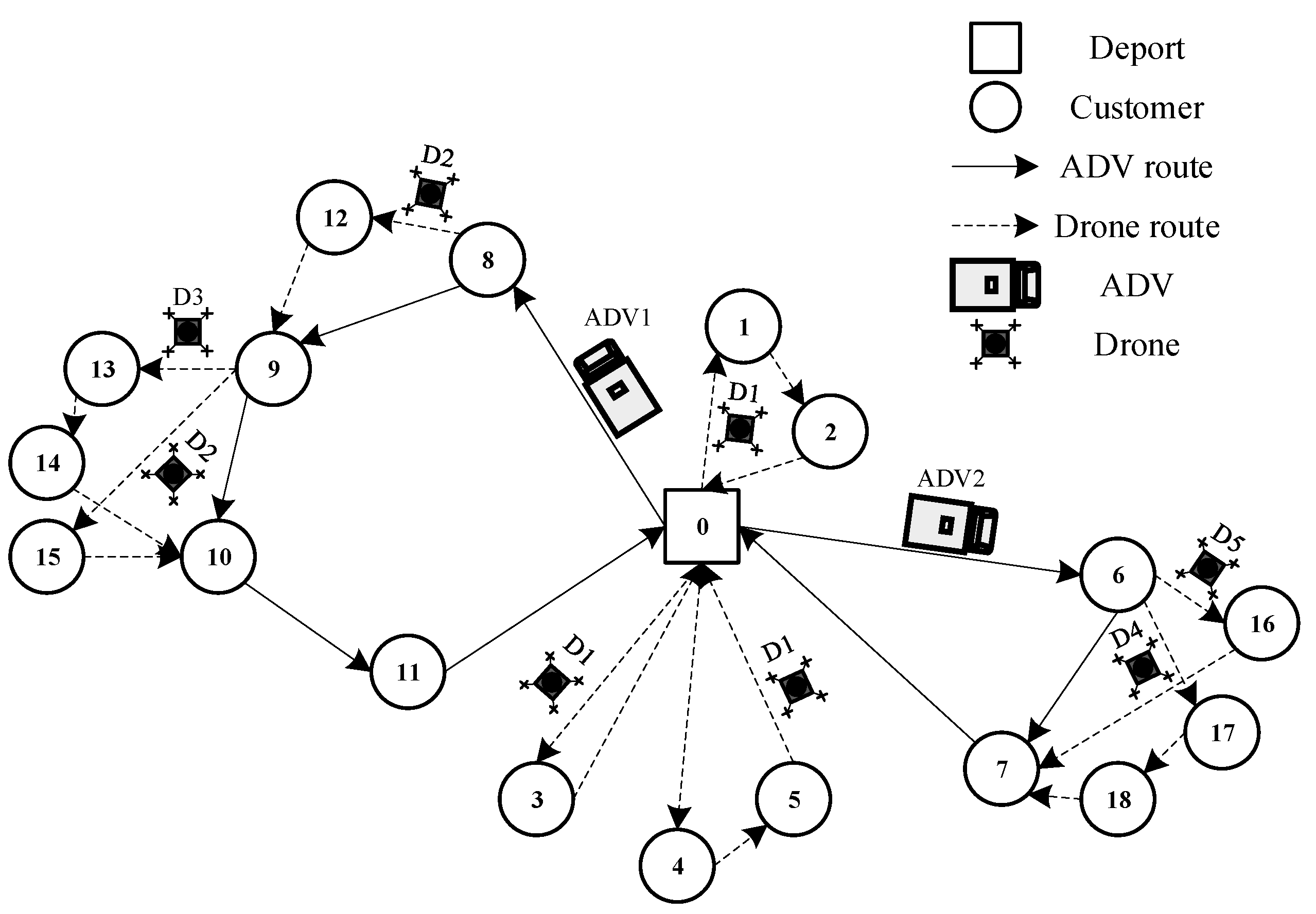
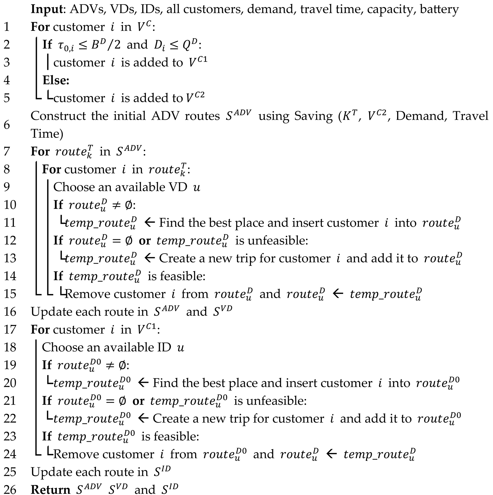
The HCWH, which is based on the saving algorithm, consists of three main components: ADV route construction (Step 2), VD route construction (Step 3), and ID route construction (Step 4). Pseudo-Code for the HCWH Algorithm is shown in Algorithm 1 and an example of the algorithm is shown in Figure 3. The algorithm follows the specific steps outlined below.

Step 1: Determine if a customer node can be serviced by an ID based on the distance from the depot node to the customer and the weight of the customer’s demand. Classify customer nodes into two sets: $V^{C1}$ for customers that can be serviced by IDs and $V^{C2}$ for customers that require collaboration between ADVs and VDs for delivery.

Step 2: Construct the local optimal ADV routes for the customers in $V^{C2}$, treating it as a Capacitated Vehicle Routing Problem (CVRP). Solve the CVRP using the Clarke and Wright saving algorithm. Then, optimize the CVRP solution using well-known local search methods such as 2-opt, swap and shift to obtain the optimal CVRP solution.

Step 3: Assign some nodes from the ADV routes to the VD routes based on the optimal CVRP solution obtained from Step 2. Construct the VD routes using the heuristic named “insert the existing routes first and create new routes second”.

Step 4: Construct the ID routes for the customers in $V^{C1}$ using the same heuristic in step 3.

Algorithm 1: Pseudo-Code for the HCWH Algorithm

4.1.1. ADV Route Construction

To construct the ADV routes for the customers in $V^{C2}$, which can be viewed as a CVRP, we employ the saving algorithm proposed by Clark and Wright along with classic neighborhood search methods such as 2-opt, swap and shift. The specific steps are as follows:

Step 1: Use the saving algorithm to construct the local optimal ADV routes, considering the constraints of capacity and maximum endurance time for the ADVs.

Step 2: Utilize classic neighborhood search methods, including 2-opt, swap, and shift, to optimize the local optimal ADV routes.

Step 3: Compare the optimized ADV routes with the local optimal ones. If the optimized ADV routes are better, adjust the local optimal ADV routes to the optimized ones and repeat Step 2. Otherwise, the optimal CVRP solution is obtained and the ADV route construction is completed.

4.1.2. VD Route Construction

To construct the VD routes, this paper applies the heuristic named “insert the existing routes first and create new routes second”. This process involves allocating some customer nodes from the ADV routes to the VD routes for delivery. The specific steps for VD route construction are as follows:

Step 1: Starting from the first customer node of each ADV route, determine whether the customer $nod{e}_i$ with demand weight can be allocated to a VD for delivery. If $nod{e}_i$ cannot be delivered by a VD, continue to the next customer node until a suitable node is found.

Step 2: If there are some existing active VD routes, try to insert $nod{e}_i$ into one of the existing active VD routes using the greedy insertion approach to minimize the distance increment of the new inserted route. Check whether the inserted VD route satisfies constraints of payload capacity, maximum endurance time and battery life. If it does, which means the insertion of $nod{e}_i$ is successful, go to Step 4; otherwise, move to Step 3.

Step 3: Determine whether $nod{e}_i$ is one of the launch or receive nodes for the existing active VD routes. If not, select an available VD and create a new VD flight with $nod{e}_i$ as a required node to be visited. The preceding and subsequent nodes in the ADV route with respect to $nod{e}_i$ become the launch node and receive node of the VD route for the new flight, respectively. Check whether the VD route for the new flight is feasible. If yes, the new VD route with $nod{e}_i$ is successfully created. Otherwise, $nod{e}_i$ remains in the ADV route.

Step 4: Repeat Steps 1–3 until all nodes in the ADV routes have been checked for potential allocation to VD routes.

4.1.3. ID Route Construction

To provide delivery service for all customers in set $V^{C1}$, the ID routes need to be constructed. The method for ID route construction is similar to VD route, following the same heuristic named “insert the existing routes first and create new routes second”. However, there are several differences between ID route construction and VD route construction:

Step 1: Select a customer $nod{e}_i$ from $V^{C1}$. If there are any existing active ID routes, try to insert $nod{e}_i$ into one of the existing active ID routes using the greedy insertion approach to minimize the distance increment of the newly inserted route.

Step 2: IDs do not need to be launched and received on the ADVs. Instead, they need to be launched and received at the depot. Each ID has a maximum working time constraint. Therefore, it is necessary to check whether the inserted ID route satisfies constraints of payload capacity, maximum endurance time and maximum working time. If it does, go to Step 4, otherwise, move to Step 3.

Step 3: Create a new flight of an available ID with $nod{e}_i$ as a required node to be visited. The ID will be launched and received at the depot in this new flight. Check whether the ID route with this new flight satisfies the constraint of maximum working time. If it does, which means the creation of the new flight is successful, go to Step 4; otherwise, reassign this new flight to another available ID until the creation of the new flight is successful.

Step 4: Repeat Steps 1–3 until all nodes in $V^{C1}$ have been assigned to IDs for delivery.

4.2. Improved Adaptive Large Neighborhood Search

Adaptive Large Neighborhood Search (ALNS), originally proposed by Ropke and Pisinger [76], has been widely used for solving VRPD problems. This approach has been adapted from the work of Ropke and Pisinger and Pisinger and Ropke [76,77]. To address the HAVDRP, we have improved the ALNS algorithm by integrating the Tabu Search algorithm and re-initialization, resulting in the IALNS algorithm.

Due to the complexity of the HAVDRP, the IALNS algorithm needs to optimize three different types of routes: ADV routes, VD routes and ID routes. If destroy and repair operators of the IALNS algorithm are designed separately for each route type, it would be challenging to design the repair operators for all types of routes. To overcome this challenge, in this paper, we combine a pair of destroy and repair operators as an optimization operator. These optimization operators are used to perform a neighborhood search for the solution. This approach not only reduces the difficulty of optimization operators design, but also allows for quantitative analysis of their performance to determine whether or not to keep them.

Furthermore, the destroy and repair process of optimization operators involves a certain degree of randomness, which potentially results in the emergence of duplicate solutions or local optima. To address this problem, the IALNS algorithm incorporates a tabu list and a re-initialization procedure within its acceptance criterion to prevent the re-search of the previously explored solutions and escape the local optima. Additionally, it reduces the weight of optimization operators that frequently result in duplicate solutions, enabling the algorithm to escape local optima more quickly. The pseudocode of Algorithm 2 illustrates the framework of the IALNS algorithm.

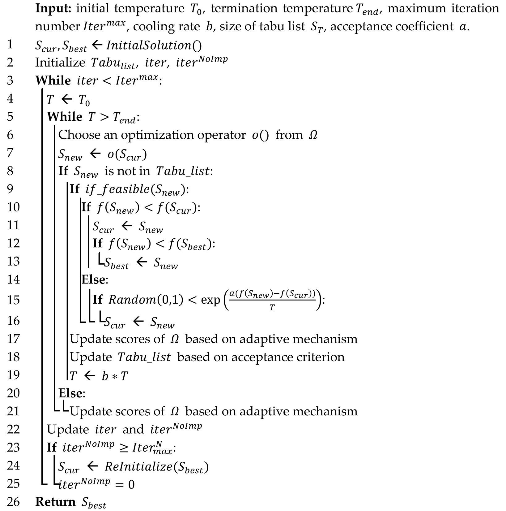
Algorithm 2: Pseudo-Code for the IALNS Algorithm

The specific steps of the IALNS algorithm are as follows:

Step 1: Input the required parameters and initialize the current solution $S_{cur}$, the best solution $S_{best}$, the number of iterations $iter$, and the initial tabu list $Tab{u}_{list}$ (Line 1–2). The initial solution is obtained by HCWH algorithm.

Step 2: Use the roulette wheel algorithm to select an optimization operator from the operator set $\Omega$ based on their weights. Use this operator to optimize the current solution $S_{cur}$, obtaining a new solution $S_{new}$ (Line 6–7).

Step 3: Check if the new solution $S_{new}$ is in the tabu list $Tab{u}_{list}$. If not, proceed to Step 4. Otherwise, update the operator weights based on the adaptive mechanism (Line 20–21) and return to Step 2 for the next optimization (Line 8).

Step 4: Determine whether to update the current solution $S_{cur}$ and the best solution $S_{best}$ based on acceptance criteria. Compare the new feasible solution $S_{new}$ with the current solution $S_{cur}$. If $S_{new}$ is better, update $S_{cur}$ to $S_{new}$; otherwise, use the Metropolis acceptance criterion to determine whether to update the current solution. If $S_{new}$ is better than the best solution $S_{best}$, update $S_{best}$ to $S_{new}$ (Line 9–16).

Step 5: Update the operator weights, the tabu list $Tab{u}_{list}$ and the current temperature $T$ (Line 17–19).

Step 6: Repeat Steps 2–5 until $T$ reaches the termination temperature $T_{end}$, completing one iteration. Update the iteration count $iter$, the iteration without improvement count $ite{r}^{NoImp}$ and reset $T$ to its initial temperature $T_0$ (Line 4–22).

Step 7: Re-initialize the current solution $S_{cur}$ and reset $ite{r}^{NoImp}$ to 0 if the best solution $S_{best}$ is not improved after $Ite{r}_{max}^N$ iterations (Line 23–25).

Step 8: Repeat Steps 2–7 until $iter$ reaches the maximum iteration number $Ite{r}^{max}$, obtaining the final best solution $S_{best}$ (Line 3–23).

4.2.1. Optimization Operators

The HAVDRP solution consists of three types of routes: ADV routes ($S^{ADV}$), VD routes ($S^{VD}$), and ID routes ($S^{ID}$). Additionally, VD routes and ID routes can be divided into sub-routes based on different flights. This paper proposes specific optimization operators for each type of route. The proposed optimization operators include:

(1)

Operators of the ADV route

Operator 1: Intra-route random removal and random insertion. Randomly remove $\sigma$ customers from a specific ADV route $R_k^T\in S^{ADV}$ ($1\le \sigma \le 0.4N$, where $N=\left|R_k^T\right|$ and $\sigma$ is an integer). Then, insert the $\sigma$ customers one by one into a random position of $R_k^T$.

Operator 2: Inter-route random removal and greedy insertion. Randomly remove $\sigma$ customers from a specific ADV route $R_{k1}^T\in S^{ADV}$, and then greedily insert these $\sigma$ customers into another ADV route $R_{k2}^T\in S^{ADV}(k2\ne k1)$ based on the shortest route distance increment.

Operator 3: Inter-route continuous removal and greedy insertion. Randomly remove a continuous set of $\sigma$ customers from a specific ADV route $R_{k1}^T\in S^{ADV}$. Then, greedily insert these $\sigma$ customers into another ADV route $R_{k2}^T\in S^{ADV}$ based on the shortest route distance increment. If the $\sigma$ customers include both the launch and receive nodes of a VD’s flight in ADV route $R_{k1}^T$, the flight is also assigned to a VD in ADV route $R_{k2}^T$. Instead, if the removal of the $\sigma$ customers breaks a VD’s flight in ADV route $R_{k1}^T$, the customer nodes in the broken flight are greedily inserted into $R_{k1}^T$.

(2)

Operator of the VD route

Operator 4: Intra-route random removal and greedy insertion. Randomly remove a customer $nod{e}_i$ from all of the VD’s sub-route where $R_{p,u}^{VD}\in S^{VD}$ ($\left|R_{p,u}^{VD}\right|\ge 4$, which means the VD $u$ serves at least 2 customers in the $p$th flight). Then, greedily insert $nod{e}_i$ back into $R_{p,u}^{VD}$ in a way that minimizes the route distance increment.

(3)

Operators between the ADV route and the VD route

Operator 5: Random removal of VD sub-route and greedy insertion into ADV route. Randomly remove all customers from a sub-route $R_{p,u}^{VD}\in S^{VD}$ in its $p$th flight of VD $u$. Then, greedily insert the removed customers into the ADV route $R_k^T\in S^{ADV}$ (the VD $u$ is carried by ADV $k$) based on the shortest route distance increment.

Operator 6: Exchange between the ADV route and the VD route. Randomly select a customer $nod{e}_i$ from a sub-route $R_{p,u}^{VD}$ of VD $u$. And randomly select a customer $nod{e}_j$ from the ADV route $R_k^T$ (the VD $u$ is carried by ADV $k$). Then, swap the positions of $nod{e}_i$ and $nod{e}_j$.

Operator 7: Random removal and greedy insertion of launch or receive nodes. Select the launch node $nod{e}_L$ or the receive node $nod{e}_R$ from a random sub-route $R_{p,u}^{VD}$ of VD $u$. Select the one that can lead to more saving after being removed for $R_k^T$. Remove $nod{e}_L$ (or $nod{e}_R$) from $R_{p,u}^{VD}$ and $R_k^T$, then greedily insert it back as a customer to be served by VD $u$ in $R_{p,u}^{VD}$. The previous one node of $nod{e}_L$ (or the next one node of $nod{e}_R$) in $R_k^T$ is employed as the new launch node (or receive node) of $R_{p,u}^{VD}$.

Operator 8: Replacement of launch or receive nodes for VD sub-routes. Randomly select a launch node $nod{e}_L\in R_k^T$ (or a receive node $nod{e}_R\in R_k^T$) for the sub-route $R_{p,u}^{VD}$ of VD $u$ (the VD $u$ is carried by ADV $k$). Replace $nod{e}_L$ (or $nod{e}_R$) with another customer node $nod{e}_j\in R_k^T$.

Operator 9: VD sub-route creation. Randomly select a customer node $nod{e}_i$ from an ADV route $R_k^T$, where $nod{e}_i$ is not a launch or receive node and it can be served by a drone. Randomly select an available VD $u$ carried by ADV $k$, and create a new sub-route $R_{p,u}^{VD}$ of VD $u$. Place $nod{e}_i$ into $R_{p,u}^{VD}$ and let VD $u$ serve $nod{e}_i$. The launch and receive node of $R_{p,u}^{VD}$ are the previous one and next one node of $nod{e}_i$ in $R_k^T$, respectively.

(4)

Operators of the ID route

Operator 10: Merge of ID sub-routes. Randomly select two sub-routes $R_{p1,u}^{ID}$ and $R_{p2,u}^{ID}$ from ID $u$. Remove $R_{p1,u}^{ID}$ from the route of ID $u$ and greedily insert the customer nodes of $R_{p1,u}^{ID}$ into $R_{p2,u}^{ID}$ based on the shortest route distance increment.

Operator 11: Split of ID sub-routes. Randomly select a sub-route $R_{p,u}^{ID}$ of ID $u$, where $\left|R_{p,u}^{ID}\right|\ge 4$. Randomly select a customer $nod{e}_i$ from $R_{p,u}^{ID}$ and create a new sub-route $R_{p1,u}^{ID}$ for ID $u$, where $nod{e}_i$ is to be serve by ID $u$ in $R_{p1,u}^{ID}$.

(5)

Operators between the ADV route and the ID route

Operator 12: Random removal of ID sub-route and greedy insertion into ADV route. Randomly remove a sub-route $R_{p,u}^{ID}$ of ID $u$. Then, greedily insert the customer nodes of $R_{p,u}^{ID}$ into an ADV route $R_k^T$.

Operator 13: Random removal from ADV route and greedy insertion into ID route. Randomly remove $\sigma$ customers from an ADV route $R_k^T$. Then, greedily insert these $\sigma$ customers into sub-routes of an ID $u$ in $S^{ID}$ based on the shortest route distance increment.

4.2.2. Feasibility Repair of the Solution

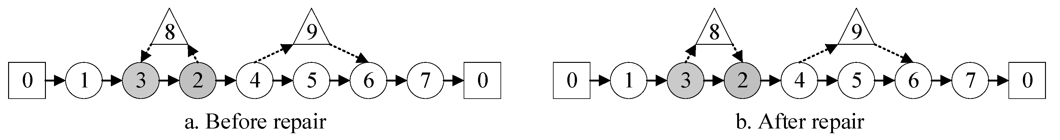
While designing the operators, the characteristics of different routes of the solution were considered. However, it is still possible to obtain some infeasible solutions during the optimization. Specifically, when optimizing the routes of ADVs, it may lead to infeasible routes for VDs. To address this issue, two feasibility repair methods are proposed.

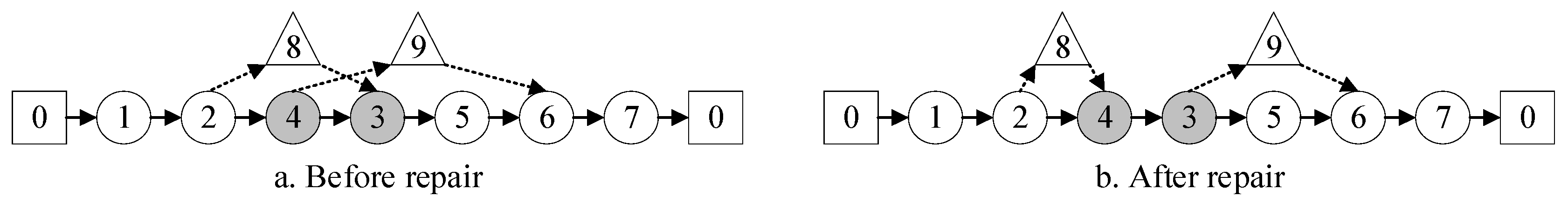
Repair Method 1: Repair the launch and receive nodes intra VD sub-route. This method corrects the order of launch and receive nodes within the same VD sub-route. In a VD sub-route, the launch node should be visited before the receive node following the sequence of the ADV route. However, the optimization may lead to an infeasible route, as depicted in Figure 4a, where the VD lands before taking off for the delivery to customer 8. To rectify this, swap the positions of the incorrectly placed launch and receive nodes. Repair method 1 is employed in this case, and the corrected outcome is illustrated in Figure 4b.

Repair Method 2: Repair the launch and receive nodes inter VD sub-routes. This method adjusts the sequence of launch and receive nodes for different flights of the same VD. In the sub-routes of different VD flights, the VD should be received in the current flight before being launched for the next flight following the sequence of the ADV route. However, the optimization might lead to an infeasible scenario, as illustrated in Figure 5a. To resolve this issue, we will swap the receive node of the current flight with the launch node of the next flight. In this case, repair method 2 is applied, and the corrected outcome is presented in Figure 5b.

It is important to note that these feasibility repair methods can correct some infeasible solutions. But there may still be violations of the assumptions and constraints of the problem. Therefore, it is still necessary to check the feasibility of new solutions based on the problem’s assumptions and constraints proposed in Section 3.

4.2.3. Adaptive Mechanism

In the HALNS algorithm, an adaptive mechanism is employed to adjust the weights of the operators. This allows for the selection of better-performing operators throughout the search process. In the IALNS algorithm, the adaptive mechanism is further improved by incorporating a tabu list. The operator weights are adjusted in cases of infeasible solutions or solutions in the tabu list, thereby enhancing the algorithm’s suitability for addressing the HAVRPD problem.

During the search process, the operator weights are adaptively adjusted based on their performance. The better an operator performs in each optimization, the greater its weight update and the higher its probability of being selected in the next optimization. The calculation of operator weights is shown in Equation (52), where $\alpha$ is the adjustment speed coefficient $(0\le \alpha \le 1)$, $i$ and $j$ donate the $i$th iteration and $j$th optimization of the $i$th iteration, $w_{i,j}$ is the weight of the operator, $S_{i,j}$ is the score of the operator, and $T_{i,j}$ is the frequency the operator is used.

$$w_{i,j+1}=\alpha \ast w_{i,j}+\left(1-\alpha \right)\ast {\displaystyle \frac{S_{i,j}}{T_{i,j}}}$$

(52)

The operator score $S_{i,j}$ can be divided into the five conditions (where $s_1>s_2>s_3>s_4>s_5$) according to the feasibility and improvement of the new solution, as is shown in

Table 3. Five conditions for the operator score.

The Score	Condition
$s_1$	$S_{new}$ is not in the tabu list. It is feasible and better than $S_{best}$.
$s_2$	$S_{new}$ is not in the tabu list. It is feasible, better than $S_{cur}$ and worse than $S_{best}$.
$s_3$	$S_{new}$ is not in the tabu list. It is feasible, worse than $S_{cur}$ and accepted to be the new current solution according to the solution acceptance criterion.
$s_4$	$S_{new}$ is not in the tabu list. It is feasible, worse than $S_{cur}$ but not accepted to be the new current solution according to the solution acceptance criterion.
$s_5$	$S_{new}$ is in the tabu list or infeasible.

.

4.2.4. Acceptance Criterion

In the IALNS algorithm, new solutions are always accepted if they are better than $S_{best}$ or $S_{cur}$. Furthermore, a simulated annealing acceptance criterion is adopted for solutions that are worse than $S_{cur}$. The probability of accepting a new solution is calculated based on Equation (53), taking the temperature and the gap of objective values into account. Accepting some worse solutions helps prevent the algorithm from getting stuck in local optima.

$$P\left(x_{new}\right)=e^{{\displaystyle \frac{-a\left(f\left(S_{new}\right)-f\left(S_{current}\right)\right)}{T}}}$$

(53)

Furthermore, in the IALNS algorithm, we introduce a re-initialization procedure to prevent the algorithm from converging to local optima. Preliminary computational experiments revealed that one of the main reasons for the algorithm’s entrapment in local optima is due to the incorrect selection of delivery methods (between ADVs or VDs) for customers. Therefore, in the IALNS algorithm, if the optimal solution has not improved after $Ite{r}_{max}^N$ iterations, the best solution $S_{best}$ is re-initialized as the new current solution to escape the local optimum. The specific steps for the re-initialization are as follows:

Step 1: Select $\sigma$ continuous customer nodes from an ADV route and place them into the set $V^{Des}$.

Step 2: In the sub-route of VDs carried by the ADV, if the launch or receive node of the sub-route is in $V^{Des}$, remove that sub-route from the VD route and greedily insert these customer nodes into the ADV route.

Step 3: Repeat the step 1~2 steps until all ADV and VD routes in $S_{best}$ have been re-initialized.

Additionally, to improve search efficiency and avoid accepting duplicate solutions, a tabu list is incorporated in the IALNS algorithm. The tabu list includes a certain number of different solutions that have been obtained in the past optimizations. When a new solution appears, the tabu list will remove the first solution in the list and place the new solution at the end, thus completing the update of the tabu list. If a new solution is in the tabu list, it will not be accepted, and the algorithm will proceed to the next optimization after updating the operator weights.

5. Computational Experiments

This section presents analyses of the proposed mathematical model and designed algorithms through computational experiments. The test instances used in this study are adapted from the Solomon benchmark, and specific details about these instances are described in Section 5.1. Section 5.2 discusses the parameter settings related to the mathematical model and algorithms. Additionally, we analyze the improvement performance of IALNS compared to the basic ALNS in Section 5.3. The performance of the designed algorithms is then studied through a series of numerical experiments in Section 5.4. In Section 5.5, we propose management suggestions for the application of ADVs and drones in last-mile delivery through sensitivity analyses. Finally, in Section 5.6, we demonstrate how the collaboration between ADVs and drones can concretely reduce total time and travel costs through a real-life case from JD.com.

The instances were solved on a computer with an Intel(R) Core (TM) i5-8250U CPU @ 1.60GHz 1.80GHz, 8.00 GB RAM, running Windows 10 on a 64-bit system. The mathematical model was solved using the Gurobi v10.0.2rc0 (win64) solver.

5.1. Benchmark Instances

While there is a considerable amount of research on the VRPD problems, there is a lack of research and standard benchmarks specifically for the VRPD problem with multiple drones and drone multi-visit. Therefore, we adapted the Solomon benchmark instances for our experiments. The Solomon instances are categorized into three sets based on the geographical locations of the customer nodes: Random (R), Clustered (C), and Random Clustered (RC). To fit the scenario and assumptions of our problem, several modifications were made to the original Solomon instances:

(1)

Time windows and service time were ignored, and only the locations and demands of customers were retained;

(2)

The X and Y coordinates of each customer node were divided by 2 (by 4 for instances over 100 customers), aligning them with the maximum endurance time of the ADVs and drones;

(3)

The customer demands were divided by 10 to comply with the maximum payload capacities of the ADVs and drones. As a result, customer demands range from 1 to 5, with some customers unable to be delivered by drones due to exceeding the maximum payload capacity.

5.2. Parameter Setting

Parameters of the unmanned equipment, such as the speed, capacity and maximum endurance time of the ADVs and drones were set based on the products of companies such as JD.com, Meituan, and Neolithic.

Table 4. Parameter setting of the unmanned equipment.

Parameters	Value
Speed of ADV $s{p}^T$(km/h)	15
Speed of drone$s{p}^D$(km/h)	60
Maximum capacity of ADV $Q^T$(kg)	200
Maximum capacity of drone$Q^D$(kg)	4.5
Maximum endurance time of ADV$B^T$(min)	480
Maximum endurance time of drone$B^D$(min)	20
Time for battery change of IDs $B^C$(min)	1
Charging rate of VDs $\mu$	1

shows the parameter settings of the unmanned equipment. The parameters of the IALNS algorithm were obtained by multiple experiments, which are presented in Appendix A.

Table 5. Parameter setting of the algorithm.

Parameters	Value
Initial temperature $T_0$	100
Termination temperature $T_{end}$	10
Cooling rate $b$	0.9886
Acceptance coefficient $a$	10
Adjustment speed coefficient $\alpha$	0.7
The number of removed customers $\sigma$	$[1, 0.4N]$
Scores of the operators [$s_1$, $s_2$, $s_3$, $s_4$, $s_5$]	[15, 12, 9, 6, 3]
Size of tabu list $S_T$	5~20
The maximum number of iterations $Ite{r}^{max}$	100~400
The maximum number of iterations without improvement $Ite{r}_{max}^N$	10~50

lists the values of the parameters, where the values of $S_T$, $Ite{r}^{max}$ and $Ite{r}_{max}^N$ are related to the scale of the instances.

5.3. Effectiveness Analysis of the IALNS Algorithm

To validate the effectiveness of the proposed IALNS algorithm relative to the basic ALNS algorithm, we performed a comparative analysis involving three algorithms: the basic ALNS algorithm, ALNS_TS algorithm, and the IALNS algorithm. The basic ALNS algorithm shares identical operators with IALNS but lacks other improvements, while ALNS_TS incorporates the improved adaptive mechanism with a tabu list, but omits the re-initialization step. The results obtained from these algorithms are shown in

Table 6. Results obtained by three algorithms.

Instance	ALNS			ALNS_TS			IALNS
	$\mathit{o}\mathit{b}{\mathit{j}}^{\mathit{b}\mathit{e}\mathit{s}\mathit{t}}$	$\mathit{o}\mathit{b}{\mathit{j}}^{\mathit{a}\mathit{v}\mathit{e}}$	${\mathit{t}}^{\mathit{a}\mathit{v}\mathit{e}}$	$\mathit{o}\mathit{b}{\mathit{j}}^{\mathit{b}\mathit{e}\mathit{s}\mathit{t}}$	$\mathit{o}\mathit{b}{\mathit{j}}^{\mathit{a}\mathit{v}\mathit{e}}$	${\mathit{t}}^{\mathit{a}\mathit{v}\mathit{e}}$	$\mathit{o}\mathit{b}{\mathit{j}}^{\mathit{b}\mathit{e}\mathit{s}\mathit{t}}$	$\mathit{o}\mathit{b}{\mathit{j}}^{\mathit{a}\mathit{v}\mathit{e}}$	${\mathit{t}}^{\mathit{a}\mathit{v}\mathit{e}}$
C101_10	72.00	72.28	14.58	72.00	72.00	19.31	72.00	72.00	17.77
C101_25	204.69	209.33	55.78	204.00	206.75	79.36	204.00	205.65	66.26
C101_50	420.59	429.88	132.06	370.40	394.69	159.54	372.19	385.32	173.46
C101_80	861.71	902.48	200.23	823.65	851.01	222.68	820.06	843.40	225.29
C101_100	971.75	1022.81	301.39	964.62	1005.13	297.26	938.86	977.89	319.58
R101_10	280.00	293.33	15.62	280.00	280.00	19.34	280.00	280.00	18.32
R101_25	472.00	494.67	62.87	472.00	493.60	69.99	472.00	477.33	51.88
R101_50	686.00	740.39	137.57	689.74	722.75	143.40	689.14	703.35	145.15
R101_80	979.13	1006.28	223.16	928.47	976.56	231.33	927.87	953.13	237.60
R101_100	1008.94	1066.67	335.96	1008.18	1035.07	346.11	993.47	1047.73	346.37
RC101_10	262.43	269.52	14.88	264.33	265.34	19.07	262.43	264.37	16.10
RC101_25	439.51	452.38	60.64	436.26	444.34	69.02	435.99	439.07	73.27
RC101_50	826.89	848.53	135.02	833.89	846.56	159.50	824.46	841.64	185.19
RC101_80	1118.98	1160.60	221.99	1071.85	1140.76	229.61	1074.85	1104.32	213.40
RC101_100	1179.89	1263.73	312.63	1181.64	1267.81	323.83	1176.71	1225.41	381.21
Average	652.30	682.19	148.29	640.07	666.82	159.29	636.27	654.71	164.72

.

Additionally, we adopted the evaluation technique proposed by AbdAllah et al. [78] to assess the performance of the three algorithms using the scoring metrics defined in Equations (54) and (55):

$$s_{i,j}={\left(1-{\displaystyle \frac{\left|f_{i,j}-B{f}_j\right|}{\beta \left|B{f}_j-W{f}_j\right|}}\right)}^p$$

(54)

$$S_{i,j}=\vartheta \sum _{j\in J}{s}_{i,j}^{best}+\left(1-\vartheta \right)\sum _{j\in J}{s}_{i,j}^{ave}$$

(55)

where $s_{i,j}$ represents the score of algorithm $i$ on instance $j$, $f_{i,j}$ denotes the objective value obtained by algorithm $i$ on instance $j$, $B{f}_j$ and $W{f}_j$ correspond to the best and worst objective values across all algorithms for instance $j$. Parameters $\beta$ (≥1) and $p$ (>1) control the scoring sensitivity: a smaller $\beta$ amplifies the score gap between optimal and worst solutions, while a larger $p$ prioritizes higher scores for near-optimal solutions. The composite score $S_{i,j}$ weighs the best-case performance ($s_{i,j}^{best}$) and average performance ($s_{i,j}^{ave}$) with a parameter $\vartheta \in \left[\mathrm{0,1}\right]$. In this study, according to AbdAllah et al. [78], $\beta$ and $p$ are set to 1.1 and 2, respectively, and $\vartheta$ is set to 0, 0.5, and 1 to evaluate different performance emphases. The final scores of three algorithms are summarized in

Table 7. Scores of three algorithms.

$\mathit{\vartheta }$	ALNS	ALNS_TS	IALNS
0	0.15	7.22	14.40
1	5.82	8.82	13.88
0.5	2.99	8.02	14.14

.

Analysis of Table 6 reveals that, across 15 instances, the IALNS algorithm achieved the best values of $ob{j}^{best}$ in 12 instances, outperforming the basic ALNS (5 instances) and ALNS_TS (6 instances). In terms of average solution quality, IALNS performed the best in 14 instances, while the other two algorithms led in only 0 and 3 instances, respectively. Furthermore, Table 7 demonstrates that the IALNS consistently attained the highest composite scores across all $\vartheta$ configurations, followed by ALNS_TS. These results confirm the efficacy of our proposed improvements in improving both solution quality and algorithmic robustness.

5.4. Results of Different Scale Instances

To evaluate the performance of the proposed algorithm, we compared the solutions obtained by HCWH and IALNS to those obtained by Gurobi in small-sized instances. For larger-sized instances where Gurobi could not find near-optimal solutions within a reasonable time, we compared the solutions obtained by IALNS to those obtained by HCWH. Through these comparisons, we demonstrated the efficacy of the IALNS algorithm for the HAVDRP problem.

The solution results for different scale instances are presented in

Table 8. Results of small-sized instances from Gurobi, HCWH and IALNS.

Instance	Gurobi		HCWH		IALNS			$\mathit{g}\mathit{a}{\mathit{p}}_1$/%	$\mathit{g}\mathit{a}{\mathit{p}}_2$/%	$\mathit{I}\mathit{m}\mathit{p}$/%
	$\mathit{o}\mathit{b}\mathit{j}$	Time/s	$\mathit{o}\mathit{b}\mathit{j}$	Time/s	$\mathit{o}\mathit{b}{\mathit{j}}^{\mathit{b}\mathit{e}\mathit{s}\mathit{t}}$	$\mathit{o}\mathit{b}{\mathit{j}}^{\mathit{a}\mathit{v}\mathit{e}}$	Time/s
c101_8	72.00	71.56	177.43	0.0033	72.00	72.00	16.77	0.00	0.00	59.42
c101_10	72.00	3600.00	186.56	0.0044	72.00	72.00	17.77	0.00	0.00	61.41
c101_15	172.00	3600.00	319.21	0.0040	172.00	172.00	18.68	0.00	0.00	46.12
c101_25	/	3600.00	418.52	0.0113	204.00	205.65	66.26	/	0.80	51.26
r101_8	280.00	8.92	346.41	0.0035	280.00	280.00	17.61	0.00	0.00	19.17
r101_10	280.00	144.72	406.41	0.0033	280.00	280.00	18.32	0.00	0.00	31.10
r101_15	/	3600.00	603.72	0.0086	380.00	380.00	22.80	/	0.00	37.06
r101_25	/	3600.00	739.56	0.0191	472.00	477.33	51.88	/	1.12	36.18
rc101_8	200.23	39.60	240.00	0.0035	200.23	201.85	15.13	0.00	0.80	16.57
rc101_10	262.43	3600.00	332.00	0.0053	262.43	264.37	16.10	0.00	0.74	20.96
rc101_15	/	3600.00	372.00	0.0085	270.43	272.44	18.64	/	0.74	27.30
rc101_25	/	3600.00	600.00	0.0402	435.99	439.07	73.27	/	0.70	27.34
Average	/	2422.07	395.15	0.0086	258.42	259.73	29.44	/	0.41	36.16

,

Table 9. Results of medium-sized instances from HCWH and IALNS.

Instance	HCWH		IALNS			$\mathit{g}\mathit{a}{\mathit{p}}_2$/%	$\mathit{I}\mathit{m}\mathit{p}$/%
	$\mathit{o}\mathit{b}\mathit{j}$	Time/s	$\mathit{o}\mathit{b}{\mathit{j}}^{\mathit{b}\mathit{e}\mathit{s}\mathit{t}}$	$\mathit{o}\mathit{b}{\mathit{j}}^{\mathit{a}\mathit{v}\mathit{e}}$	Time/s
c101_30	464.25	0.01	208.00	209.22	85.48	0.58	55.20
c101_50	779.42	0.09	372.19	385.32	138.77	3.41	52.25
c101_60	1035.42	0.23	515.71	524.53	152.11	1.68	50.19
c101_80	1513.71	0.53	820.06	843.40	180.23	2.77	45.82
r101_30	767.41	0.04	500.00	510.67	63.66	2.09	34.85
r101_50	1099.95	0.13	689.14	703.35	116.12	2.02	37.35
r101_60	1254.99	0.52	701.61	727.94	162.23	3.62	44.09
r101_80	1696.42	1.41	927.87	953.13	190.08	2.65	45.30
rc101_30	900.00	0.08	715.99	731.02	74.62	2.06	20.45
rc101_50	1044.00	0.28	824.46	841.64	148.15	2.04	21.03
rc101_60	1432.73	0.75	916.87	956.59	125.74	4.15	36.01
rc101_80	1972.70	1.26	1074.85	1104.32	170.72	2.67	45.51
Average	1163.42	0.39	688.89	707.59	167.49	2.48	40.67

and

Table 10. Results of large-sized instances from HCWH and IALNS.

Instance	HCWH		IALNS			$\mathit{g}\mathit{a}{\mathit{p}}_2$/%	Imp/%
	$\mathit{o}\mathit{b}\mathit{j}$	Time/s	$\mathit{o}\mathit{b}{\mathit{j}}^{\mathit{b}\mathit{e}\mathit{s}\mathit{t}}$	$\mathit{o}\mathit{b}{\mathit{j}}^{\mathit{a}\mathit{v}\mathit{e}}$	Time/s
c101_100	1641.71	1.05	938.86	977.89	319.58	3.99	42.81
c101_120	1621.14	2.10	879.64	922.72	383.49	4.67	45.74
c101_150	1761.73	4.33	984.40	1016.60	862.52	3.17	44.12
c101_200	2040.02	12.87	1094.66	1127.45	967.76	2.91	46.34
r101_100	1814.08	2.80	993.47	1047.73	346.37	5.18	45.24
r101_120	2164.38	4.46	1120.36	1161.35	362.78	3.53	48.24
r101_150	2284.48	11.51	1207.81	1241.19	901.66	2.69	47.13
r101_200	2650.21	20.00	1563.70	1589.90	791.06	1.65	41.00
rc101_100	2156.31	3.37	1176.71	1225.41	381.21	3.97	45.43
rc101_120	2013.30	4.30	854.33	898.43	379.79	4.91	57.57
rc101_150	2042.22	7.51	1036.95	1077.79	846.24	3.79	49.22
rc101_200	2551.61	20.19	1253.39	1296.36	948.25	3.31	50.88
Average	2061.77	8.61	1092.02	1131.90	624.23	3.65	46.98

. In these tables, “$obj$” and “Time” denote the objective value and solving time, respectively. For the IALNS algorithm results, “$ob{j}^{best}$” and “$ob{j}^{ave}$” represent the best and average objective values over 10 runs, while the solving time is the average value of 10 runs. “$ga{p}_1$” and “$ga{p}_2$” indicate the gaps between “$ob{j}^{best}$” of IALNS and “$obj$” of Gurobi, as well as the gaps between “$ob{j}^{best}$” and “$ob{j}^{ave}$” of IALNS, respectively. “$Imp$” signifies the improvements for “$ob{j}^{best}$” of IALNS compared to “$obj$” of HCWH.

The results in Table 8 show that for instances with a scale of 10 or less, Gurobi can obtain the optimal solution. However, as the scale of the instances increases, Gurobi’s solving time also significantly increases and it becomes challenging to obtain optimal values within the one-hour constraint. The values of $ga{p}_1$ indicate that IALNS achieves near-optimal solutions for the majority of instances. Additionally, all the $ga{p}_2$ values are less than 1.2%, with an average of 0.41%, suggesting that the IALNS algorithm maintains good stability for small-sized instances. Furthermore, IALNS shows significant improvements compared to the initial solutions obtained by HCWH, with average improvements of 54.55%, 30.88%, and 23.04% across C, R, and RC instances, respectively. Although HCWH has a faster solving time, taking less than 0.1 s for small-sized instances, IALNS takes longer but most of them still completes within 1.2 min, with an average solving time of 29.44 s. Thus, IALNS provides superior solutions within short time for small-sized instances.

Results for medium and large-sized instances are shown in Table 9 and Table 10. In medium-sized instances, IALNS outperforms HCWH across C, R, and RC instances, with average improvements of 50.87%, 40.40%, and 30.75%, respectively. The average value of $ga{p}_2$ is 2.48%, indicating that IALNS maintains stable performance in medium-sized instances. HCWH also demonstrates fast solving time, with an average of 0.45 s for medium-sized instances. IALNS has a longer average solving time of 133.99 s but still yields satisfactory solutions within a reasonable time. For large-sized instances, IALNS continues to achieve substantial optimization, with an average improvement of 44.75%, 45.40%, and 50.77% over HCWH across C, R, and RC instances. The average value of $ga{p}_2$ is 3.65%, affirming good result stability. HCWH has an average solving time of 7.87 s, while IALNS takes 428.62 s. Considering the scale of instances and the complexity of the HAVDRP problem, these solving times are considered acceptable.

5.5. Sensitivity Analyses of Key Parameters

5.5.1. The Number of VDs

To assess the impact of the number of VDs on the total time of HAVDRP, a sensitivity analysis was conducted. Three instances with 100 customers were used for this analysis, and each ADV carried 1 to 5 VDs for delivery. The results (average value over 10 runs) are shown in Figure 6. As expected, it can be observed that increasing the number of VDs can significantly reduce the total time. However, this impact shows diminishing marginal returns, which is particularly evident in instances with dispersed customer distributions like r101_100 and rc101_100. This is because the VDs have limited endurance so that they can only serve a limited number of customers. Therefore, the best number of VDs needs to be determined based on a comprehensive assessment of factors such as drone endurance, customer distribution, and operating cost of VDs.

5.5.2. The Charging Rate of VDs

In the HAVDRP, VDs require recharging on ADVs to extend their endurance time. To investigate the impact of charging rates on total time, a sensitivity analysis was conducted with charging rates ranging from 0 to 2. The results are illustrated in Figure 7. As shown in Figure 7, the total time decreases as the charging rate increases; however, this relationship exhibits a clear diminishing marginal return. Specifically, the total time stabilizes when the charging rate reaches 1. This suggests that further increases in charging capacity beyond this threshold yield diminishing improvements in system efficiency. Considering the trade-off between investment costs for drone recharging infrastructure and the benefits of reduced total time, the optimal charging rate for this study is determined to be approximately 1. This value achieves a balance between operational efficiency gains and resource allocation constraints, as higher charging rates would require disproportionate investments without proportionate reductions in total time.

5.5.3. The Maximum Endurance Time and Capacity of Drones

In the VRPD literature, it is widely assumed that a drone can only deliver a single package per flight [52]. However, our research enables drones to serve multiple customers within the endurance time and capacity constraints. To analyze the impact of these two parameters on total time, we conducted a sensitivity analysis using three benchmark instances: c101_50, r101_50, and rc101_50. The results, averaged across these instances, are presented in Figure 8. As depicted in Figure 8, the total time decreases as both the maximum payload capacity and endurance time increase. However, this relationship exhibits a diminishing marginal return effect. Moreover, there exists an interdependency between payload and endurance time. For instance, when the drone’s maximum endurance time is constrained to 10 min, increasing payload capacity yields minimal reductions in total time. Therefore, managers must balance the incremental costs of improving payload/endurance against the marginal time savings. For example, investing in higher payload capacity may be inefficient if endurance is already constrained.

5.5.4. The Speed of Drones

With the advancement of technology, the maximum speed of drones is increasing, while the speed of ADVs is limited by traffic safety considerations. Many countries regulate the speed of ADVs, such as 15 km/h or 20 km/h, to ensure the safety of pedestrians and vehicles. To analyze the impact of drone speed on the total time of HAVDRP, we conducted a sensitivity analysis experiment, varying drone speed from 30 km/h to 90 km/h while maintaining the maximum flight distance. The results are shown in Figure 9.

According to Figure 9, enhancing drone speed from 30 km/h to 75 km/h effectively reduces the total delivery time. However, surpassing 75 km/h may not necessarily result in further time reduction. This is because ADVs travel on roads by Manhattan distances while drones fly in the air by Euclidean distance, and ADVs are always slower than drones. Therefore, ADVs typically require VDs to wait at the receive nodes. When the drone speed is 30 km/h, some ADVs may still have to wait for VDs at some of the receive nodes. But when the speed is 75 km/h, there may not be significant time savings with further speed increases. Moreover, augmenting drone speed adds complexity to problem-solving, as the algorithm must determine the optimal delivery method for customers: by IDs or through the collaboration between ADVs and VDs.

5.5.5. The Parameters of ID

In the hybrid delivery scenario involving ADVs and drones, utilizing VDs for customer service can effectively reduce the total time. However, the impact of using IDs remains unclear. Therefore, we conducted a sensitivity analysis experiment using three different types of IDs with varying parameters to explore their impact on the total time. Specifically, drones ID_1, ID_2 and ID_3 were selected to represent small, medium and large sized IDs, respectively. Their parameters are shown in

Table 11. The parameters of three types of ID.

Parameter	VD	ID
		$\mathit{I}{\mathit{D}}_1$	$\mathit{I}{\mathit{D}}_2$	$\mathit{I}{\mathit{D}}_3$
Speed of drone $s{p}^D$/(km/h)	60	60	60	60
Maximum capacity of drone $Q^D$/(kg)	4.5	4.5	7.5	10
Maximum endurance time of drone $B^D$/(min)	20	20	25	30

. Also, ID_0 indicates that IDs are not used for delivery. These drones were tested on three instances with 100 customers, and the results are presented in Figure 10. In Figure 10, V%, VD% and ID% represent the proportion of customers served by ADVs, VDs and IDs, respectively. The “obj” represents the objective values obtained by HCWH algorithm, and the “obj_ave” represents the average objective values obtained by IALNS algorithm over 10 runs.

According to Figure 10a, we can find that employing larger-sized IDs can increase the percentage usage of IDs, but it does not necessarily reduce the total time. According to Figure 10b, in the solutions obtained by IALNS, the proportion of IDs usage consistently remains within a very low range and the total time remains essentially constant. On the other hand, the solutions optimized by IALNS show a significant decrease in the percentage usage of IDs compared to the initial solutions, while the percentage usage of VDs significantly increases. The increase in maximum capacity and maximum endurance time of IDs leads to more usage of IDs but cannot reduce the total time. This suggests that the delivery method using ADVs and VDs is more effective for minimizing the total time compared to using IDs. However, IDs have advantages such as lower costs and faster reactions to urgent orders. Therefore, if considering minimizing cost or urgent orders for customers, using IDs for delivery is still a viable and effective method.

5.5.6. The Maximum Capacity of ADVs

To investigate the impact of ADV’s maximum payload capacity on total time, we conducted a sensitivity analysis by varying the maximum capacity from 50 kg to 250 kg. The results are presented in Figure 11. According to Figure 11, across all test instances, increasing the ADV’s maximum payload capacity from 50 kg to 100 kg leads to a significant reduction in total time, especially in the instances of c101_100 and rc101_100. However, beyond 100 kg, the total time stabilizes, indicating diminishing returns. This stabilization occurs because the limiting factor shifts from the ADV’s payload capacity to its maximum endurance time constraint. In our problem scenario, the current maximum payload capacity of 200 kg is sufficient for operational requirements. If further improvements of ADV are sought to improve delivery efficiency, efforts should focus on increasing the maximum endurance time rather than payload capacity.

5.6. Case Analysis

The data for this case were obtained from JD.com, encompassing 1 depot and 20 customers. The spatial distribution of all nodes is illustrated in Figure 12, where the depot is marked in red and customers in blue. For this case study, we utilized AutoNavi Map software to obtain the actual driving distances between nodes for ADVs and the Euclidean distances for drone flights. This section analyzes the differences in total time and travelling costs between two systems: (1) an ADV-only system without drones, and (2) an integrated ADV-Drone system. Based on the cost parameters proposed by Jiang et al. [62], the unit costs per kilometer for trucks and drones were set at 1 and 0.2, respectively. Additionally, based on the findings of Sharpe and Basma [79], which suggest that ADV costs are approximately 85–90% of truck costs, we assigned an ADV cost of 0.9 per kilometer.

The delivery routes and detailed results for both systems are presented in Figure 13 and

Table 12. The results of ADV-Drone system and ADV-Only system.

System	Route	Total Time/min	Traveling Cost
ADV-Drone	ADV Route: 0→9→5→19→13→20→8→18→0; VD#1 Route: 0→3→14→5, 20→4→12→8, 18→11→0; VD#2 Route: 0→2→1→10→9, 13→7→8, 18→6→15→0; ID Route: 0→16→17→0;	320.75	92.68
ADV-Only	ADV#1 Route: 0→11→18→7→6→12→4→20→13→19→5→8→14→10→9→15→3→1→2→0; ADV#2 Route: 0→16→17→0;	545.10	122.65

. In Figure 13, the ADV routes are represented by black and green lines, while the routes of VD#1 and VD#2 are indicated by orange and blue lines, and the route of ID#1 is represented by red lines. As shown in Table 12, the ADV-Drone system utilized 1 ADV, 2 VDs, and 1 ID, whereas the ADV-Only system required 2 ADVs. And the ADV-Drone system achieved a 41.16% reduction in total time and reducing travelling costs by 24.44% compared to the ADV-only system. This improvement stems from the reduced reliance on ADVs and a significant decrease in their travel distances due to drone deployment. By offloading some of the delivery tasks to drones, the ADV-Drone system optimized resource allocation and path planning, thereby achieving the dual objectives of reducing time and enhancing cost efficiency.

6. Conclusions

Intelligent logistics is a growing trend in last-mile delivery, and the integration of ADVs and drones has emerged as a popular research topic in recent years. This paper presents a new last-mile delivery model that combines ADVs and drones, providing a theoretical foundation for automated last-mile logistics. The key contributions of this paper are as follows:

First, a novel variant of the Vehicle Routing Problem with Drones (VRPD) is introduced, referred to as the Hybrid Autonomous Vehicle and Drone Routing Problem (HAVDRP). This problem takes into account three delivery tools: autonomous delivery vehicles (ADVs), ADV-carried drones (VDs) and independent drones (IDs). Second, a Mixed Integer Programming (MIP) model is developed for the HAVDRP, considering that each ADV carries multiple drones and drones can serve multiple customers in a single flight. The model also addresses synchronization and battery constraints between ADVs and multiple VDs, ensuring its relevance to practical applications. Third, two algorithms are designed to solve the HAVDRP, and the improved performance of IALNS algorithm compared with the basic ALNS algorithm is verified through computational experiments. Finally, the experimental comparisons with the Gurobi solver in small-sized instances are conducted to demonstrate the effectiveness of the designed algorithms. For large-scale problems, the proposed algorithms can provide high-quality solutions for instances with up to 200 customers. Moreover, sensitivity analysis experiments are conducted to propose management recommendations, providing valuable insights for decision-makers in the application of hybrid delivery with ADVs and drones.

Based on this work, future research on the hybrid delivery problem involving ADVs and drones could include: (1) Considering multiple depots to deliver to customers or utilizing heterogeneous fleets of ADVs and drones with varying capacities; (2) Conducting a more detailed energy consumption analysis for ADVs and drones, taking into account the effects of their payload and road conditions; (3) Exploring the possibility of not limiting the launch and receive nodes for ADVs and drones to customer nodes or depots and considering the addition of the drone docking points to increase the proportion of customers served by drones. This would leverage the low cost and high speed of the drone delivery to further improve the efficiency of last-mile logistics. (4) Incorporating dynamic orders into the HAVDRP to align research scenarios more closely with real-world applications.

References

1. Thibbotuwawa, A.; Bocewicz, G.; Nielsen, P.; Banaszak, Z. Unmanned Aerial Vehicle Routing Problems: A Literature Review. Appl. Sci. 2020, 10, 4504. [Google Scholar] [CrossRef]
2. Alamouri, A.; Lampert, A.; Gerke, M. Impact of Drone Regulations on Drone Use in Geospatial Applications and Research: Focus on Visual Range Conditions, Geofencing and Privacy Considerations. PFG—J. Photogramm. Remote Sens. Geoinf. Sci. 2023, 91, 381–389. [Google Scholar] [CrossRef]
3. Gao, J.; Zhen, L.; Laporte, G.; He, X. Scheduling Trucks and Drones for Cooperative Deliveries. Transp. Res. Part E Logist. Transp. Rev. 2023, 178, 103267. [Google Scholar] [CrossRef]
4. Liang, Y.-J.; Luo, Z.-X. A Survey of Truck–Drone Routing Problem: Literature Review and Research Prospects. J. Oper. Res. Soc. China 2022, 10, 343–377. [Google Scholar] [CrossRef]
5. Włodzimierz, C.; Iwona, G. Autonomous Vehicles in Urban Agglomerations. Transp. Res. Procedia 2019, 40, 655–662. [Google Scholar] [CrossRef]
6. Kapser, S.; Abdelrahman, M. Acceptance of Autonomous Delivery Vehicles for Last-Mile Delivery in Germany—Extending UTAUT2 with Risk Perceptions. Transp. Res. Part C Emerg. Technol. 2020, 111, 210–225. [Google Scholar] [CrossRef]
7. AlKheder, S.; Bash, A.; Al Baghli, Z.; Al Hubaini, R.; Al Kader, A. Customer Perception and Acceptance of Autonomous Delivery Vehicles in the State of Kuwait during COVID-19. Technol. Forecast. Soc. Change 2023, 191, 122485. [Google Scholar] [CrossRef] [PubMed]
8. Figliozzi, M.A. Carbon Emissions Reductions in Last Mile and Grocery Deliveries Utilizing Air and Ground Autonomous Vehicles. Transp. Res. Part Transp. Environ. 2020, 85, 102443. [Google Scholar] [CrossRef]
9. Lemardelé, C.; Estrada, M.; Pagès, L.; Bachofner, M. Potentialities of Drones and Ground Autonomous Delivery Devices for Last-Mile Logistics. Transp. Res. Part E Logist. Transp. Rev. 2021, 149, 102325. [Google Scholar] [CrossRef]
10. Scherr, Y.O.; Neumann Saavedra, B.A.; Hewitt, M.; Mattfeld, D.C. Service Network Design with Mixed Autonomous Fleets. Transp. Res. Part E Logist. Transp. Rev. 2019, 124, 40–55. [Google Scholar] [CrossRef]
11. Liu, D.; Deng, Z.; Mao, X.; Yang, Y.; Kaisar, E.I. Two-Echelon Vehicle-Routing Problem: Optimization of Autonomous Delivery Vehicle-Assisted E-Grocery Distribution. IEEE Access 2020, 8, 108705–108719. [Google Scholar] [CrossRef]
12. Farahani, M.; Zegordi, S.H.; Kashan, A.H. A Tailored Meta-Heuristic for the Autonomous Electric Vehicle Routing Problem Considering the Mixed Fleet. IEEE Access 2023, 11, 8207–8222. [Google Scholar] [CrossRef]
13. Ulmer, M.W.; Streng, S. Same-Day Delivery with Pickup Stations and Autonomous Vehicles. Comput. Oper. Res. 2019, 108, 1–19. [Google Scholar] [CrossRef]
14. Yu, J.J.Q. Two-Stage Request Scheduling for Autonomous Vehicle Logistic System. IEEE Trans. Intell. Transp. Syst. 2019, 20, 1917–1929. [Google Scholar] [CrossRef]
15. Nasri, M.I.; Bektaş, T.; Laporte, G. Route and Speed Optimization for Autonomous Trucks. Comput. Oper. Res. 2018, 100, 89–101. [Google Scholar] [CrossRef]
16. Bray, G.; Cebon, D. Selection of Vehicle Size and Extent of Multi-Drop Deliveries for Autonomous Goods Vehicles: An Assessment of Potential for Change. Transp. Res. Part E Logist. Transp. Rev. 2022, 164, 102806. [Google Scholar] [CrossRef]
17. Li, B.; Liu, S.; Tang, J.; Gaudiot, J.-L.; Zhang, L.; Kong, Q. Autonomous Last-Mile Delivery Vehicles in Complex Traffic Environments. Computer 2020, 53, 26–35. [Google Scholar] [CrossRef]
18. Moradi, N.; Sadati, İ.; Çatay, B. Last Mile Delivery Routing Problem Using Autonomous Electric Vehicles. Comput. Ind. Eng. 2023, 184, 109552. [Google Scholar] [CrossRef]
19. Wang, J.; Pan, J.; Zheng, L.; Tan, X. A Systematic Space-Time Route Planning Approach Coordinated With Task Assignment for Autonomous Delivery Vehicles Fleet. IEEE Access 2023, 11, 79370–79383. [Google Scholar] [CrossRef]
20. Abbas, N.; Abbas, Z.; Liu, X.; Khan, S.S.; Foster, E.D.; Larkin, S. A Survey: Future Smart Cities Based on Advance Control of Unmanned Aerial Vehicles (UAVs). Appl. Sci. 2023, 13, 9881. [Google Scholar] [CrossRef]
21. Silva, A.T.; Duarte, S.P.; Melo, S.; Witkowska-Konieczny, A.; Giannuzzi, M.; Lobo, A. Attitudes towards Urban Air Mobility for E-Commerce Deliveries: An Exploratory Survey Comparing European Regions. Aerospace 2023, 10, 536. [Google Scholar] [CrossRef]
22. Moshref-Javadi, M.; Winkenbach, M. Applications and Research Avenues for Drone-Based Models in Logistics: A Classification and Review. Expert Syst. Appl. 2021, 177, 114854. [Google Scholar] [CrossRef]
23. Dang, S.; Liu, Y.; Luo, Z.; Liu, Z.; Shi, J. A Survey of the Routing Problem for Cooperated Trucks and Drones. Drones 2024, 8, 550. [Google Scholar] [CrossRef]
24. Murray, C.C.; Chu, A.G. The Flying Sidekick Traveling Salesman Problem: Optimization of Drone-Assisted Parcel Delivery. Transp. Res. Part C Emerg. Technol. 2015, 54, 86–109. [Google Scholar] [CrossRef]
25. Carlsson, J.G.; Song, S. Coordinated Logistics with a Truck and a Drone. Manag. Sci. 2018, 64, 4052–4069. [Google Scholar] [CrossRef]
26. Agatz, N.; Bouman, P.; Schmidt, M. Optimization Approaches for the Traveling Salesman Problem with Drone. Transp. Sci. 2018, 52, 965–981. [Google Scholar] [CrossRef]
27. Dell’Amico, M.; Montemanni, R.; Novellani, S. Drone-Assisted Deliveries: New Formulations for the Flying Sidekick Traveling Salesman Problem. Optim. Lett. 2021, 15, 1617–1648. [Google Scholar] [CrossRef]
28. Boccia, M.; Masone, A.; Sforza, A.; Sterle, C. A Column-and-Row Generation Approach for the Flying Sidekick Travelling Salesman Problem. Transp. Res. Part C Emerg. Technol. 2021, 124, 102913. [Google Scholar] [CrossRef]
29. Amorosi, L.; Puerto, J.; Valverde, C. Coordinating Drones with Mothership Vehicles: The Mothership and Drone Routing Problem with Graphs. Comput. Oper. Res. 2021, 136, 105445. [Google Scholar] [CrossRef]
30. El-Adle, A.M.; Ghoniem, A.; Haouari, M. A Variable Neighborhood Search for Parcel Delivery by Vehicle with Drone Cycles. Comput. Oper. Res. 2023, 159, 106319. [Google Scholar] [CrossRef]
31. Jeong, H.Y.; Song, B.D.; Lee, S. Truck-Drone Hybrid Delivery Routing: Payload-Energy Dependency and No-Fly Zones. Int. J. Prod. Econ. 2019, 214, 220–233. [Google Scholar] [CrossRef]
32. Cho, Y.H.; Baek, D.; Chen, Y.; Jung, M.J.; Vinco, S.; Macii, E.; Poncino, M. Multi-Criteria Coordinated Electric Vehicle-Drone Hybrid Delivery Service Planning. IEEE Trans. Veh. Technol. 2023, 72, 5892–5905. [Google Scholar] [CrossRef]
33. Tamke, F.; Buscher, U. The Vehicle Routing Problem with Drones and Drone Speed Selection. Comput. Oper. Res. 2023, 152, 106112. [Google Scholar] [CrossRef]
34. Tu, P.A.; Dat, N.T.; Dung, P.Q. Traveling Salesman Problem with Multiple Drones. In Proceedings of the Ninth International Symposium on Information and Communication Technology—SoICT 2018, Da Nang, Vietnam, 6–7 December 2018; ACM Press: Danang City, Viet Nam, 2018; pp. 46–53. [Google Scholar]
35. Karak, A.; Abdelghany, K. The Hybrid Vehicle-Drone Routing Problem for Pick-up and Delivery Services. Transp. Res. Part C Emerg. Technol. 2019, 102, 427–449. [Google Scholar] [CrossRef]
36. Murray, C.C.; Raj, R. The Multiple Flying Sidekicks Traveling Salesman Problem: Parcel Delivery with Multiple Drones. Transp. Res. Part C Emerg. Technol. 2020, 110, 368–398. [Google Scholar] [CrossRef]
37. Raj, R.; Murray, C. The Multiple Flying Sidekicks Traveling Salesman Problem with Variable Drone Speeds. Transp. Res. Part C Emerg. Technol. 2020, 120, 102813. [Google Scholar] [CrossRef]
38. Leon-Blanco, J.M.; Gonzalez-R, P.L.; Andrade-Pineda, J.L.; Canca, D.; Calle, M. A Multi-Agent Approach to the Truck Multi-Drone Routing Problem. Expert Syst. Appl. 2022, 195, 116604. [Google Scholar] [CrossRef]
39. Deng, X.; Guan, M.; Ma, Y.; Yang, X.; Xiang, T. Vehicle-Assisted UAV Delivery Scheme Considering Energy Consumption for Instant Delivery. Sensors 2022, 22, 2045. [Google Scholar] [CrossRef]
40. Moshref-Javadi, M.; Hemmati, A.; Winkenbach, M. A Comparative Analysis of Synchronized Truck-and-Drone Delivery Models. Comput. Ind. Eng. 2021, 162, 107648. [Google Scholar] [CrossRef]
41. Tiniç, G.O.; Karasan, O.E.; Kara, B.Y.; Campbell, J.F.; Ozel, A. Exact Solution Approaches for the Minimum Total Cost Traveling Salesman Problem with Multiple Drones. Transp. Res. Part B Methodol. 2023, 168, 81–123. [Google Scholar] [CrossRef]
42. Betti Sorbelli, F.; Corò, F.; Das, S.K.; Palazzetti, L.; Pinotti, C.M. On the Scheduling of Conflictual Deliveries in a Last-Mile Delivery Scenario with Truck-Carried Drones. Pervasive Mob. Comput. 2022, 87, 101700. [Google Scholar] [CrossRef]
43. Sacramento, D.; Pisinger, D.; Ropke, S. An Adaptive Large Neighborhood Search Metaheuristic for the Vehicle Routing Problem with Drones. Transp. Res. Part C Emerg. Technol. 2019, 102, 289–315. [Google Scholar] [CrossRef]
44. Chiang, W.-C.; Li, Y.; Shang, J.; Urban, T.L. Impact of Drone Delivery on Sustainability and Cost: Realizing the UAV Potential through Vehicle Routing Optimization. Appl. Energy 2019, 242, 1164–1175. [Google Scholar] [CrossRef]
45. Wang, D.; Hu, P.; Du, J.; Zhou, P.; Deng, T.; Hu, M. Routing and Scheduling for Hybrid Truck-Drone Collaborative Parcel Delivery with Independent and Truck-Carried Drones. IEEE Internet Things J. 2019, 6, 10483–10495. [Google Scholar] [CrossRef]
46. Lei, D.; Cui, Z.; Li, M. A Dynamical Artificial Bee Colony for Vehicle Routing Problem with Drones. Eng. Appl. Artif. Intell. 2022, 107, 104510. [Google Scholar] [CrossRef]
47. Kuo, R.J.; Lu, S.-H.; Lai, P.-Y.; Mara, S.T.W. Vehicle Routing Problem with Drones Considering Time Windows. Expert Syst. Appl. 2022, 191, 116264. [Google Scholar] [CrossRef]
48. Huang, S.-H.; Huang, Y.-H.; Blazquez, C.A.; Chen, C.-Y. Solving the Vehicle Routing Problem with Drone for Delivery Services Using an Ant Colony Optimization Algorithm. Adv. Eng. Inform. 2022, 51, 101536. [Google Scholar] [CrossRef]
49. Wei, S.; Fan, H.; Ren, X.; Diao, X. Time-Dependent Vehicle Routing Problem with Drones Under Vehicle Restricted Zones and No-Fly Zones. Appl. Sci. 2025, 15, 2207. [Google Scholar] [CrossRef]
50. Zang, X.; Jiang, L.; Liang, C.; Dong, J.; Lu, W.; Mladenovic, N. Optimization Approaches for the Urban Delivery Problem with Trucks and Drones. Swarm Evol. Comput. 2022, 75, 101147. [Google Scholar] [CrossRef]
51. Gu, R.; Poon, M.; Luo, Z.; Liu, Y.; Liu, Z. A Hierarchical Solution Evaluation Method and a Hybrid Algorithm for the Vehicle Routing Problem with Drones and Multiple Visits. Transp. Res. Part C Emerg. Technol. 2022, 141, 103733. [Google Scholar] [CrossRef]
52. Imran, N.M.; Mishra, S.; Won, M. A-VRPD: Automating Drone-Based Last-Mile Delivery Using Self-Driving Cars. IEEE Trans. Intell. Transp. Syst. 2023, 24, 9599–9612. [Google Scholar] [CrossRef]
53. Ren, X.-X.; Fan, H.-M.; Bao, M.-X.; Fan, H. The Time-Dependent Electric Vehicle Routing Problem with Drone and Synchronized Mobile Battery Swapping. Adv. Eng. Inform. 2023, 57, 102071. [Google Scholar] [CrossRef]
54. Wang, X.; Poikonen, S.; Golden, B. The Vehicle Routing Problem with Drones: Several Worst-Case Results. Optim. Lett. 2017, 11, 679–697. [Google Scholar] [CrossRef]
55. Schermer, D.; Moeini, M.; Wendt, O. A Matheuristic for the Vehicle Routing Problem with Drones and Its Variants. Transp. Res. Part C Emerg. Technol. 2019, 106, 166–204. [Google Scholar] [CrossRef]
56. Wang, Z.; Sheu, J.-B. Vehicle Routing Problem with Drones. Transp. Res. Part B Methodol. 2019, 122, 350–364. [Google Scholar] [CrossRef]
57. Rave, A.; Fontaine, P.; Kuhn, H. Drone Location and Vehicle Fleet Planning with Trucks and Aerial Drones. Eur. J. Oper. Res. 2023, 308, 113–130. [Google Scholar] [CrossRef]
58. Kitjacharoenchai, P.; Min, B.-C.; Lee, S. Two Echelon Vehicle Routing Problem with Drones in Last Mile Delivery. Int. J. Prod. Econ. 2020, 225, 107598. [Google Scholar] [CrossRef]
59. Zhou, H.; Qin, H.; Cheng, C.; Rousseau, L.-M. An Exact Algorithm for the Two-Echelon Vehicle Routing Problem with Drones. Transp. Res. Part B Methodol. 2023, 168, 124–150. [Google Scholar] [CrossRef]
60. Lin, M.; Chen, Y.; Han, R.; Chen, Y. Discrete Optimization on Truck-Drone Collaborative Transportation System for Delivering Medical Resources. Discret. Dyn. Nat. Soc. 2022, 2022, 1811288. [Google Scholar] [CrossRef]
61. Luo, Q.; Wu, G.; Trivedi, A.; Hong, F.; Wang, L.; Srinivasan, D. Multi-Objective Optimization Algorithm With Adaptive Resource Allocation for Truck-Drone Collaborative Delivery and Pick-Up Services. IEEE Trans. Intell. Transp. Syst. 2023, 24, 9642–9657. [Google Scholar] [CrossRef]
62. Jiang, J.; Dai, Y.; Yang, F.; Ma, Z. A Multi-Visit Flexible-Docking Vehicle Routing Problem with Drones for Simultaneous Pickup and Delivery Services. Eur. J. Oper. Res. 2024, 312, 125–137. [Google Scholar] [CrossRef]
63. Faiz, T.I.; Vogiatzis, C.; Noor-E-Alam, M. Computational Approaches for Solving Two-Echelon Vehicle and UAV Routing Problems for Post-Disaster Humanitarian Operations. Expert Syst. Appl. 2024, 237, 121473. [Google Scholar] [CrossRef]
64. Dell’Amico, M.; Montemanni, R.; Novellani, S. Matheuristic Algorithms for the Parallel Drone Scheduling Traveling Salesman Problem. Ann. Oper. Res. 2020, 289, 211–226. [Google Scholar] [CrossRef]
65. Lei, D.; Chen, X. An Improved Variable Neighborhood Search for Parallel Drone Scheduling Traveling Salesman Problem. Appl. Soft Comput. 2022, 127, 109416. [Google Scholar] [CrossRef]
66. Mbiadou Saleu, R.G.; Deroussi, L.; Feillet, D.; Grangeon, N.; Quilliot, A. An Iterative Two-step Heuristic for the Parallel Drone Scheduling Traveling Salesman Problem. Networks 2018, 72, 459–474. [Google Scholar] [CrossRef]
67. Li, Y.; Zhang, G.; Pang, Z.; Li, L. Continuum Approximation Models for Joint Delivery Systems Using Trucks and Drones. Enterp. Inf. Syst. 2020, 14, 406–435. [Google Scholar] [CrossRef]
68. Schermer, D.; Moeini, M.; Wendt, O. The Traveling Salesman Drone Station Location Problem. In Optimization of Complex Systems: Theory, Models, Algorithms and Applications; Le Thi, H.A., Le, H.M., Pham Dinh, T., Eds.; Advances in Intelligent Systems and Computing; Springer International Publishing: Cham, Switzerland, 2020; Volume 991, pp. 1129–1138. ISBN 978-3-030-21802-7. [Google Scholar]
69. Ham, A.M. Integrated Scheduling of M-Truck, m-Drone, and m-Depot Constrained by Time-Window, Drop-Pickup, and m-Visit Using Constraint Programming. Transp. Res. Part C Emerg. Technol. 2018, 91, 1–14. [Google Scholar] [CrossRef]
70. Montemanni, R.; Dell’Amico, M. Constraint Programming Models for the Parallel Drone Scheduling Vehicle Routing Problem. EURO J. Comput. Optim. 2023, 11, 100078. [Google Scholar] [CrossRef]
71. Ulmer, M.W.; Thomas, B.W. Same-day Delivery with Heterogeneous Fleets of Drones and Vehicles. Networks 2018, 72, 475–505. [Google Scholar] [CrossRef]
72. Ramos, T.R.P.; Vigo, D. A New Hybrid Distribution Paradigm: Integrating Drones in Medicines Delivery. Expert Syst. Appl. 2023, 234, 120992. [Google Scholar] [CrossRef]
73. Nguyen, M.A.; Dang, G.T.-H.; Hà, M.H.; Pham, M.-T. The Min-Cost Parallel Drone Scheduling Vehicle Routing Problem. Eur. J. Oper. Res. 2022, 299, 910–930. [Google Scholar] [CrossRef]
74. Mbiadou Saleu, R.G.; Deroussi, L.; Feillet, D.; Grangeon, N.; Quilliot, A. The Parallel Drone Scheduling Problem with Multiple Drones and Vehicles. Eur. J. Oper. Res. 2022, 300, 571–589. [Google Scholar] [CrossRef]
75. Macrina, G.; Di Puglia Pugliese, L.; Guerriero, F.; Laporte, G. Drone-Aided Routing: A Literature Review. Transp. Res. Part C Emerg. Technol. 2020, 120, 102762. [Google Scholar] [CrossRef]
76. Ropke, S.; Pisinger, D. An Adaptive Large Neighborhood Search Heuristic for the Pickup and Delivery Problem with Time Windows. Transp. Sci. 2006, 40, 455–472. [Google Scholar] [CrossRef]
77. Pisinger, D.; Ropke, S. A General Heuristic for Vehicle Routing Problems. Comput. Oper. Res. 2007, 34, 2403–2435. [Google Scholar] [CrossRef]
78. AbdAllah, A.M.F.M.; Essam, D.L.; Sarker, R.A. On Solving Periodic Re-Optimization Dynamic Vehicle Routing Problems. Appl. Soft Comput. 2017, 55, 1–12. [Google Scholar] [CrossRef]
79. Sharpe, B.; Basma, H. A Meta-Study of Purchase Costs for Zero-Emission Trucks; International Council on Clean Energy Transportation: Washington, DC, USA, 2022. [Google Scholar]
80. Chen, C.; Demir, E.; Huang, Y. An Adaptive Large Neighborhood Search Heuristic for the Vehicle Routing Problem with Time Windows and Delivery Robots. Eur. J. Oper. Res. 2021, 294, 1164–1180. [Google Scholar] [CrossRef]
81. Mulumba, T.; Najy, W.; Diabat, A. The Drone-Assisted Pickup and Delivery Problem: An Adaptive Large Neighborhood Search Metaheuristic. Comput. Oper. Res. 2024, 161, 106435. [Google Scholar] [CrossRef]
Figure 1. An example diagram of HAVDRP.
Drones 09 00280 g001
Figure 2. The components of the mathematical model.
Drones 09 00280 g002
Figure 3. Example of HCWH Algorithm.
Drones 09 00280 g003
Figure 4. An example of repair method 1.
Drones 09 00280 g004
Figure 5. An example of repair method 2.
Drones 09 00280 g005
Figure 6. Results of solutions with different numbers of VDs.
Drones 09 00280 g006
Figure 7. Results of solutions with different charging rates of VDs.
Drones 09 00280 g007
Figure 8. Results of solutions with various maximum endurance times and capacities of drones.
Drones 09 00280 g008
Figure 9. Results of solutions with various speeds of drones.
Drones 09 00280 g009
Figure 10. Results of solutions with three types of ID.
Drones 09 00280 g010
Figure 11. Results of solutions with various maximum capacities of ADVs.
Drones 09 00280 g011
Figure 12. All nodes distribution map.
Drones 09 00280 g012
Figure 13. The delivery routes of ADV-Drone System and ADV-Only System.
Drones 09 00280 g013