Enhancing Integrated Navigation with a Self-Attention LSTM Hybrid Network for UAVs in GNSS-Denied Environments

Abstract

Performing long-duration navigation without the global navigation satellite system (GNSS) network is a challenging task, particularly for small unmanned aerial vehicles (UAVs) equipped with low-cost micro-electro-mechanical sensors. This study proposes a hybrid neural network that integrates self-attention mechanisms with long short-term memory (SALSTM) to enhance GNSS-denied navigation performance. The estimation task of GNSS-denied navigation is first modeled based on UAV aerodynamics and kinematics, enabling a precise definition of the inputs and outputs that SALSTM needs to map. A self-attention layer is inserted in multiple LSTM layers to capture long-range dependencies in subtle dynamic changes. The output layer is designed to generate state sequences, leveraging the recursive nature of LSTM to enforce state continuity constraints. The outputs of SALSTM are fused to enhance integrated navigation within an extended Kalman filter framework. The performance of the proposed method is evaluated using flight data obtained from field tests. The results demonstrate that SALSTM-enhanced integrated navigation achieves superior long-term stability and improves velocity and position estimation accuracy by more than 50% compared to the best existing methods.

1. Introduction

Navigation in GNSS-denied environments has become a key research focus due to potential signal blockage and interference. In classical methods, inertial navigation systems (INSs) and global navigation satellite systems (GNSSs) are two of the most well-established navigation methods [1]. INSs can carry high-frequency measurements and estimates, but their errors accumulate due to consistent bias and noise in rapid measurement. GNSS has no cumulative errors and is used to correct INS estimates in the Kalman filter framework [2]. Satellite-denied navigation is particularly challenging for small unmanned aerial vehicles (SUAVs), as they usually use low-cost micro-electro-mechanical sensors (MEMSs) as the measurement unit for INS, which usually possess greater measurement noise and errors. Numerous researchers have tried to introduce different techniques to fix these problems.

The integration of additional sensors is a widely adopted strategy to enhance navigation in GNSS-denied environments. Common methods include utilizing external observation base stations [3,4], fusing information from communication base stations [5] or ultra-wideband (UWB) systems [6,7], and adopting simultaneous localization and mapping (SLAM) to achieve independent navigation [8]. While these solutions can increase navigation accuracy if implemented with care, higher cost and complexity are inevitable byproducts of additional sensor usage [9]. In addition, these methods still have issues in base station-less, large-scale outdoor, and map-less environments [7,8].

In recent years, neural networks have been an important technical solution revolutionizing navigation techniques [10]. Some earlier studies used radial basis function (RBF) neural networks to produce expected values during GNSS outages [11,12]. Follow-up studies have shown that multi-layer perceptron [13] (MLP) can effectively increase the robustness of INS/GNSS techniques. The mentioned networks suffer from poor generalizability in high-noise situations and cannot store prior information and extract dynamical patterns between their inputs [14]. Recurrent neural networks (RNNs) are more capable of capturing and learning the sequential characteristics of dynamic models. Further research has proposed methods aided by RNNs to improve positional accuracy, with INS and RNNs integrated in a loosely coupled manner [15]. A similar study also used RNNs to provide velocity and position increments in a GNSS-denied environment, with tests conducted on a boat [16]. Other networks that use sequence data as input are recurrent fuzzy wavelet neural networks (RFWNNs). RFWNNs have an enhanced ability to deal with uncertainty, nonlinearity, and complex signals and have been utilized to characterize dynamic model, position, and velocity errors based on current and past information [17].

However, the learning gradient of networks that use RNNs to model recursive features vanishes exponentially [18], making it difficult to effectively utilize long sequence data. Considering the mentioned problems, the focus of later studies has been on using a long short-term memory (LSTM) network to aid in GNSS-denied navigation [19,20,21,22]. LSTM introduces cell states and gating mechanisms to control the flow of information, enabling the capture of time-series features of its inputs during longer intervals. Gated Recurrent Units (GRUs) share a similar mechanism with LSTM and have become a focal point of applied research in recent years [23,24]. Compared to LSTM, GRUs achieve higher computational efficiency through a simplified architecture but sacrifice certain long-term memory capabilities inherent to LSTM. In recent studies, attention mechanisms have been combined with LSTM to extract signal autocorrelation and cross-correlation [1]. In addition, stacking convolutional layers with the LSTM/GRU layers is believed to capture spatial and temporal structures buried hidden inside the INS data [14,25,26].

Some studies have also developed deep reinforcement learning frameworks based on LSTM for perception and control in unknown or dynamic environments, which is an end-to-end navigation and guidance approach but does not explicitly perform state estimation [27,28,29]. Following LSTM, the self-attention mechanism was proposed and became central to transformer architectures, primarily for parallelization and scalability [30,31]. This mechanism weighs the importance of different parts of an input sequence when performing inference and computes attention scores between all positions in the sequence, enabling the model to capture long-range dependencies.

So far, scholars have focused on using and improving neural networks with different architectures to assist in navigation and have achieved good application results. However, according to our survey, few existing methods have modeled this estimation problem in GNSS-denied environments. Most studies have attempted to directly employ neural networks as pseudo-GNSSs to provide position and velocity measurements [19,20,21,22]. However, neural networks face challenges in effectively capturing the weak correlation between inertial measurements and position. Achieving this requires not only a substantial volume of training data but also the use of highly complex network architectures [14]. Even so, mapping such subtle relationships may introduce unnecessary errors.

As shown in Figure 1, the estimation task is first modeled based on UAV aerodynamics when GNSS is denied in this study. Based on this model, the corresponding inputs and outputs of the neural network are carefully selected, thereby avoiding invalid mappings. Meanwhile, we designed a new self-attention and LSTM (SALSTM) hybrid network to improve the inference performance when the dynamic of the UAV is not well motivated. The self-attention layer is inserted in multiple LSTM layers. Thus, through the LSTM layer, both input and output sequences maintain recursive properties, which is crucial for preserving the model’s dynamic continuity constraints of UAVs. Finally, real-time SALSTM inference of attitude and velocity is fused for integrated navigation in the extended Kalman filter (EKF) framework, which can provide long-term stable attitude and velocity estimation and improve position estimation accuracy.

The organization of this paper is described as follows. Section 2 presents the aerodynamics of UAVs and establishes an optimization model for navigation estimation without GNSS. Section 3 introduces the SALSTM-enhanced navigation method for GNSS-denied environments, including the data fusion approach in Section 3.2 and the design of the SALSTM architecture in Section 3.3. In Section 4, the proposed method is evaluated using data collected from fixed-wing UAV field flight tests. Section 5 summarizes this study and indicates directions for future work.

2. Estimation Model

Interpretability/explainability is one of the essential issues of machine learning, as it relates to the extremely important issue of safety assurance (related to navigation) [18]. Artificial neural networks model the system as a black box, rendering the selection of input and output variables critically important. Improperly defined input and output configurations can introduce noise and even prevent the training process from converging. To enhance the inference accuracy and robustness of SALSTM, this study analyzes the flight dynamics and kinematics of UAVs and establishes a velocity and attitude estimation model for GNSS-denied environments. Based on the analysis, appropriate input and output sequences are selected, and an optimized neural network architecture was designed.

2.1. Aerodynamics of UAVs

For fixed-wing UAVs equipped with inertial sensors, it is impossible to directly obtain unbiased position, attitude, and velocity measurements from inertial data when GNSS is denied. On the other hand, the relative velocity (${\mathit{V}}_r$) of a UAV to the surrounding airmass determines the aerodynamic forces (${\mathit{F}}_a$), while ${\mathit{V}}_r$ depends on the ground velocity ($\mathit{V}$) and the Euler attitude ($\mathit{\xi }$). Since ${\mathit{F}}_a$ can be calculated from inertial measurements, this section first analyzes the relationship among inertial measurements ($\mathit{V}$ and $\mathit{\xi }$). The reference frames associated with this relationship are illustrated in Figure 2. Below, superscript $b$ denotes values in the body frame, and $n$ denotes values in the navigation frame.

First, the relationship between inertial measurements and aerodynamic force is expressed as follows:

$$m{\mathit{f}}_{sf}^b=m\left({\mathit{a}}^b-{\mathit{C}}_n^b{\mathit{g}}^n\right)={\mathit{F}}_T^b+C_a^b{\mathit{F}}_a+{\mathit{C}}_n^b{\mathit{G}}^n$$

(1)

where $m$ is the mass of the UAV, ${\mathit{f}}_{sf}$ is the specific force measured by inertial sensors, $\mathit{a}$ is the acceleration relative to the ground, ${\mathit{C}}_n^b$ is the rotation matrix from the navigation frame to the body frame, $\mathit{g}$ is gravitational acceleration, ${\mathit{F}}_T^b$ is thrust, ${\mathit{C}}_a^b$ is the rotation matrix from the wind frame to the body frame, $\mathit{G}$ is gravity.

Secondly, the simplified aerodynamic force in Equation (1) is given in Ref. [32], where derivatives relative to rudder deflection and angular velocity are disregarded, as these states change at high frequencies. When defined in the wind frame, the aerodynamic force is denoted as follows:

$$\begin{array}{c}{\mathit{F}}_a=\left[\begin{array}{c}-D\\ Y\\ -L\end{array}\right]=\overline{Q}S\left[\begin{array}{c}-\left(C_{D_0}+C_{D_{{\alpha }^2}}{\alpha }^2\right)\\ C_{Y_{\beta }}\beta \\ -\left(C_{L_0}+C_{L_{\alpha }}\alpha \right)\end{array}\right]\end{array}$$

(2)

where $\overline{Q}$ is the dynamic pressure, $S$ is the reference area, $\alpha$ is the angle of attack, $\beta$ is the sideslip angle, $C_{D_0}$ is the drag coefficient when $\alpha =0$, $C_{D_{{\alpha }^2}}$ represents the change in drag coefficient with respect to ${\alpha }^2$, $C_{Y_{\beta }}$ represents the change in the coefficient of lateral force with respect to $\beta$, $C_{L_0}$ is the lift coefficient when $\alpha =0$, and $C_{L_{\alpha }}$ represents the change in the lift coefficient with respect to $\alpha$.

Variables $\overline{Q}$, $\beta$, and $\alpha$ in Equation (2) are defined based on the relative velocity in the body frame as follows:

$$\begin{array}{l}{V}_a=\parallel {\mathit{V}}_r^b\parallel \\ \alpha ={\tan }^{-1}\left(w/u\right)\\ \beta ={\sin }^{-1}\left(v/V_a\right)\\ \overline{Q}=0.5\rho V_a^2\end{array}$$

(3)

where $V_a$ is the airspeed; $u$, $v$, and $w$ are components of ${\mathit{V}}_r^b$ along the x, y, and z-axes, respectively, in the body frame; and $\rho$ denotes air density.

Finally, according to the definition of a so-called “wind triangle”, ${\mathit{V}}_r^b$ is related to the attitude, ground velocity, and wind velocity (${\mathit{V}}_w$) as Equation (4). Here, the attitude is represented in the form of a rotation matrix ($C_n^b$).

$${\mathit{V}}_r^b=C_n^b\left[{\mathit{V}}^n-{\mathit{V}}_w^n\right]$$

(4)

2.2. State Dynamics

The system state is time-continuous and exhibits recursive characteristics. The states (${\mathbf{x}}^{\mathbf{*}}$) are the attitude denoted by Euler angles and the ground velocity in the navigation frame. The parameters (${\mathbf{p}}^{\mathbf{*}}$) are the aerodynamic derivatives, reference area, mass, wind velocity, and geomagnetic vector. The states are to be estimated, and parameters are thought to be either constant or slowly changing.

$${\mathbf{x}}^{\mathbf{*}}=\left[\begin{array}{c}\mathit{\xi }\\ {\mathit{V}}^n\end{array}\right]$$

(5)

$${\mathbf{p}}^{\mathbf{*}}={\left[C_{L_0},C_{L_{\alpha }},C_{Y_{\beta }},S,m,{\mathit{V}}_w^n,{\mathit{M}}_I^n\right]}^T$$

(6)

where ${\mathit{M}}_I^n$ is the geomagnetic vector in the navigation frame.

The input data include angular rates $\mathit{\omega }$ and ${\mathit{f}}_{sf}$ as follows:

$${\mathbf{u}}^{\mathbf{*}}=\left[\begin{array}{c}\mathit{\omega }\\ {\mathit{f}}_{\mathit{s}\mathit{f}}\end{array}\right]$$

(7)

The state transition function is expressed as follows:

$${\mathbf{f}}^{\mathbf{*}}\left({\mathbf{x}}^{\mathbf{*}},{\mathbf{u}}^{\mathbf{*}}\right)=\left[\begin{array}{c}\dot{\mathit{\xi }}\\ {\dot{\mathit{V}}}^n\end{array}\right]=\left[\begin{array}{c}{T}_r\mathit{\omega }\\ C_b^n{\mathit{f}}_{sf}+\mathit{g}\end{array}\right]$$

(8)

where $C_b^n={\left(C_n^b\right)}^T$ and $T_r$ is constructed by the roll angle ($\varphi$) and pitch angle ($\theta$) as follows:

$$T_r=\left[\begin{array}{ccc}1& \sin \varphi \sin \theta /\cos \theta & \cos \varphi \sin \theta /\cos \theta \\ 0& \cos \varphi & -\sin \varphi \\ 0& \sin \varphi /\cos \theta & \cos \varphi /\cos \theta \end{array}\right]$$

(9)

Then, the predicted state is expressed as follows:

$${\mathbf{x}}_{k+1}^{\mathrm{*}}={\mathbf{x}}_k^{\mathrm{*}}+T_s·\mathbf{f}\left({\mathbf{x}}_k^{\mathbf{*}},{\mathbf{u}}_k^{\mathbf{*}}\right)+{\mathsf{\nu }}_{{\mathbf{x}}^{\mathbf{*}},k}$$

(10)

where subscript $k$ denotes values at time $t_k$, $T_s$ is the sampling interval, and ${\mathsf{\nu }}_{{\mathbf{x}}^{\mathbf{*}},k}$ is process noise of ${\mathbf{x}}^{\mathbf{*}}$.

Consider the following parameter:

$${\mathbf{p}}_{k+1}^{\mathrm{*}}={\mathbf{p}}_k^{\mathrm{*}}+{\mathsf{\nu }}_{{\mathbf{p}}^{\mathbf{*}},k}$$

(11)

where ${\mathsf{\nu }}_{{\mathbf{p}}^{\mathbf{*}},k}$ is process noise of ${\mathbf{p}}^{\mathbf{*}}$.

2.3. Observation Model

Measurements used to correct the system state are the measured airspeed, the specific force measured by inertial sensors, and magnetic intensity. The measurement vector is expressed as follows:

$${\mathbf{z}}^{\mathit{*}}={\left[V_p,f^y,f^z,M_x,M_y,M_z\right]}^T$$

(12)

where $V_p$ is the pitot airspeed, $f^y$ and $f^z$ denote components of ${\mathit{f}}_{sf}$ along the x and y-axes, respectively, in the body frame; and $M^x$, $M^y$, and $M^z$ represent the three-axis magnetic field intensity (${\mathit{M}}_{mag}$) measured by the magnetometer.

The time-varying measurement equations are expressed as follows:

$${\mathbf{z}}^{\mathrm{*}}={\mathbf{h}}^{*}\left({\mathbf{x}}^{\mathbf{*}},{\mathbf{u}}^{\mathbf{*}}\right)+{\mathit{\eta }}_{{\mathbf{z}}^{*}}$$

(13)

where ${\mathit{\eta }}_{{\mathbf{z}}^{*}}$ is the measurement noise.

As shown in Equation (14), the first measurement equation uses the definition of airspeed to relate the measured airspeed to the relative velocity. The second and third measurement equations use the y and z-accelerometer, together with the aerodynamic model, to estimate velocity and attitude. Measurement Equations (4)–(6) utilize measurements from the magnetometer and the geomagnetic vector to estimate heading.

$${\mathbf{h}}^{\mathbf{*}}\left({\mathbf{x}}^{\mathbf{*}},{\mathbf{u}}^{\mathbf{*}}\right)=\left[\begin{array}{c}\parallel u,v,w\parallel \\ {\displaystyle \frac{v}{u}}{C}_{Y_{\beta }}\overline{Q}S\cos {\displaystyle \frac{v}{u}}/m\\ \left({\displaystyle \frac{w}{u}}{C}_{L_{\alpha }}+C_{L_0}\right)\overline{Q}S\cos {\displaystyle \frac{w}{u}}/m\\ C_n^b{\mathit{M}}_I\end{array}\right]+{\mathsf{\lambda }}^{\mathbf{*}}$$

(14)

where ${\left[u,v,w\right]}^T=C_n^b\left({\mathit{V}}^n-{\mathit{V}}_w^n\right)$ and ${\mathsf{\lambda }}^{\mathbf{*}}$ is the approximation error within the models, which is assumed to be white Gaussian noise. For simplicity, when flow angles $\alpha$ and $\beta$ are small, the following approximations are made: $\alpha \approx w/u,\beta \approx v/u,C_a^b\approx \mathrm{d}\mathrm{i}\mathrm{a}\mathrm{g}\left[\sin \alpha ,\cos \alpha ,\cos \beta \right]$.

2.4. Moving Horizon Estimation

Moving horizon estimation of the state (${\mathbf{x}}^{\mathbf{*}}$) can be achieved by leveraging both the state dynamics and observation models of the system. This process involves constructing the objective function (Equation (15)) based on the observed model and establishing time-continuous constraints (Equation (16)) based on the state transition function.

$$J\left({\mathbf{x}}_i^{*},{\mathbf{p}}_i^{*},{\mathbf{u}}_i^{*}\right)=\underset{\begin{array}{c}{\mathbf{x}}_i^{*}\\ {\mathbf{p}}_i^{*}\end{array}}{\min }\left({‖\begin{array}{c}{\mathbf{x}}_{k-n}^{\mathbf{*}}-{\widehat{\mathbf{x}}}_{k-n}^{*}\\ {\mathbf{p}}_{k-n}^{\mathrm{*}}-{\widehat{\mathbf{p}}}_{k-n}^{*}\end{array}‖}^2+\sum _{i=k-n}^k{‖{{\mathbf{z}}^{\mathrm{*}}}_i-{\mathbf{h}}^{\mathbf{*}}\left({\mathbf{x}}_i^{*},{\mathbf{u}}_i^{*}\right)‖}^2\right)$$

(15)

$$\left\{\begin{array}{c}{\mathbf{x}}_{i+1}^{*}-{\mathbf{x}}_i^{*}=0.5·T_s·\left[\mathbf{f}\left({\mathbf{x}}_{i+1}^{*},{\mathbf{u}}_{i+1}^{*}\right)+\mathbf{f}\left({\mathbf{x}}_i^{*},{\mathbf{u}}_i^{*}\right)\right]\\ {\mathbf{p}}_{i+1}^{\mathrm{*}}-{\mathbf{p}}_i^{\mathrm{*}}-{\mathit{\nu }}_{{\mathit{p}}_{\mathit{i}}}^{\mathrm{*}}=\mathbf{0}\end{array}\right.$$

(16)

Given the definitions of ${\mathbf{x}}^{\mathbf{*}}$, ${\mathbf{p}}^{\mathbf{*}}$, ${\mathbf{u}}^{\mathbf{*}}$, and the measurement equations, it is evident that the objective function is continuous. Additionally, the domains of ${\mathbf{x}}^{\mathbf{*}}$ and ${\mathbf{p}}^{\mathbf{*}}$ are compact sets. According to the Weierstrass theorem, the objective function is bounded, and a globally optimal solution exists.

Nevertheless, due to the complex dynamics and kinematics of UAVs, the objective function exhibits highly nonlinear characteristics, rendering high-frequency online optimization extremely challenging. However, by leveraging the easily accessible flight data from UAVs, this optimization problem can be transformed into a regression problem. Specifically, neural networks can be trained to map sequences ${\mathbf{u}}_i^{*}$ and ${{\mathbf{z}}^{\mathrm{*}}}_i$ to ${\mathbf{x}}_i^{*}$, instead of directly solving the objective function.

3. Methodology

As analyzed in Section 2, since neural networks can be used to model the relationship between measurements and attitude/velocity, we propose the integration of a neural network into an integrated navigation system to enhance navigation performance. On one hand, neural networks struggle to infer navigation states in real time at a sufficiently high frequency; on the other hand, the framework of integrated navigation allows for the fusion of more diverse information, thereby improving the robustness of the navigation system.

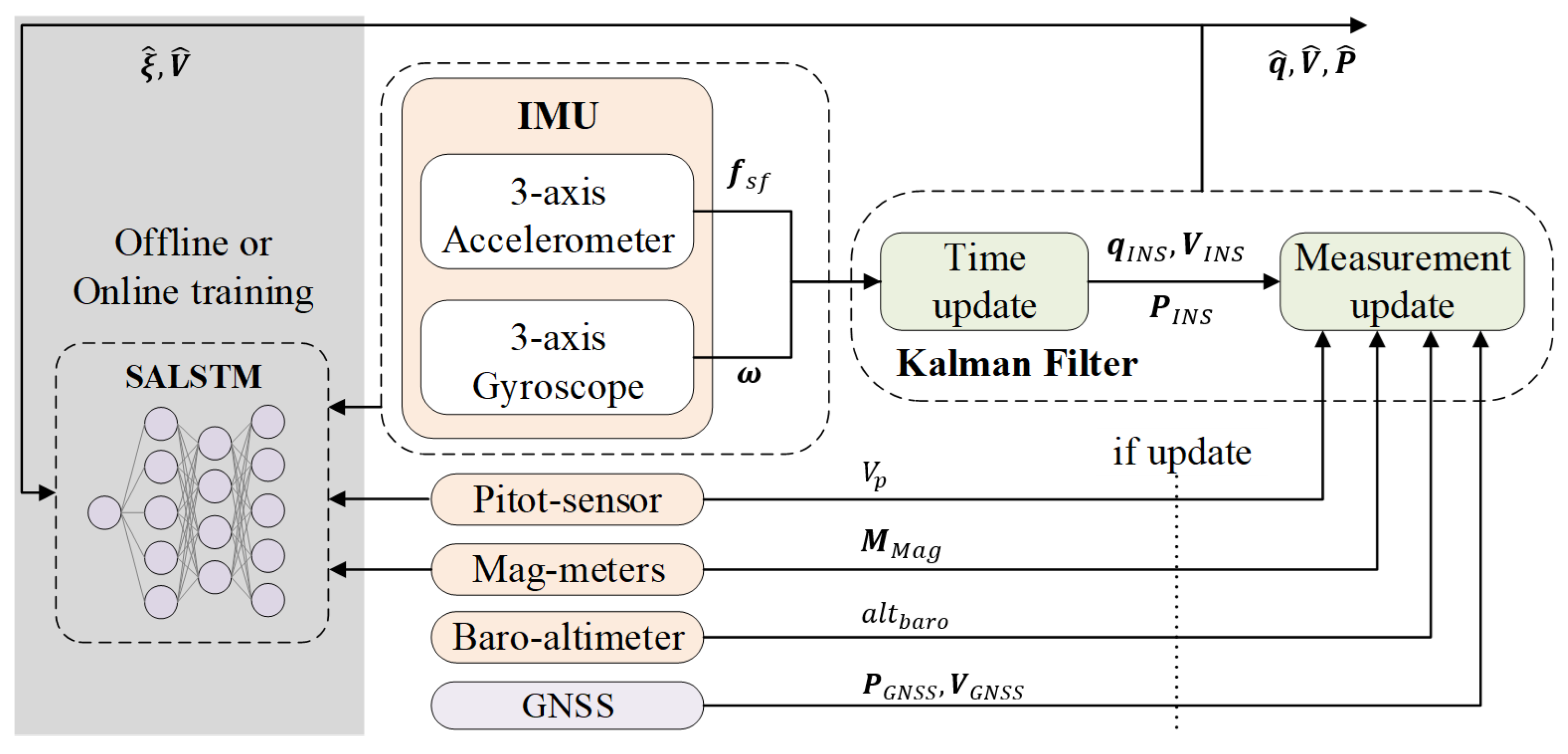
3.1. Integrated Navigation Framework

Sensor configurations for navigation in small UAVs typically include GNSS, MEMS-based Inertial Measurement Units (MIMUs), barometric altimeters, pitot airspeed sensors, and magnetometers. These sensors are largely applicable to most environmental conditions and are, therefore, widely used as a basic sensor suite. The integrated navigation system based on the above sensors provides position, attitude, and velocity estimation using a Kalman filter for information fusion (as shown in Figure 3).

When GNSS is available, the MIMU’s ${\mathit{f}}_{sf}$ and $\mathit{\omega }$, pitot airspeed ($V_p$), barometer altitude ($al{t}_{baro}$), magnetic field intensity measured by the magnetometer (${\mathit{M}}_{mag}$), GNSS velocity (${\mathit{V}}_{GNSS}$), and ${\mathit{P}}_{GNSS}$ are fused for navigation. Then, the ${\mathit{f}}_{sf}$, $\mathit{\omega }$, $V_p$, ${\mathit{M}}_{mag}$, and estimated Euler attitude ($\widehat{\mathit{\xi }}$) and ground velocity ($\widehat{\mathit{V}}$) are captured and used to train the designed neural network.

The selection of these training data is based on the estimation model described in Section 2, where ${\mathit{f}}_{sf}$ and $\mathit{\omega }$ are used to construct ${\mathbf{u}}^{\mathrm{*}}$; $f^{b,y},f^{b,z}$ $V_p$, and ${\mathit{M}}_{mag}$ are used to construct ${\mathbf{z}}^{\mathrm{*}}$; and $\widehat{\mathit{\xi }}$ and $\widehat{\mathit{V}}$ serve as the optimal ${\mathbf{x}}^{\mathrm{*}}$.

As shown in Figure 4, when GNSS is denied, there is no need to solve the objective function (Equation (15)) to provide attitude and velocity measurements. The Euler attitude (${\mathit{\xi }}_{nn}$) and velocity (${\mathit{V}}_{nn}$, denoted by subscript “$nn$”) output by SALSTM are considered optimal, that is, based on the moving-horizon sequence data of ${\mathit{f}}_{sf}$, $\mathit{\omega }$, $V_p$, and ${\mathit{M}}_{mag}$, the well-trained SALSTM infers ${\mathit{\xi }}_{nn}$, and ${\mathit{V}}_{nn}$ in real time to assist with navigation.

In the Kalman filter framework, the vehicle’s attitude (${\mathit{q}}_{INS}$), velocity (${\mathit{V}}_{INS}$), and relative position (${\mathit{P}}_{INS}$) are first estimated based on the IMU’s accelerometers and gyroscope (subscripted as “INS”) [33]. Next, $V_p$, $al{t}_{baro}$, ${\mathit{\xi }}_{nn}$, and ${\mathit{V}}_{nn}$ are fused as measurements to correct the estimates. As data of magnetometers have already been used to infer ${\mathit{\xi }}_{nn}$ and ground ${\mathit{V}}_{nn}$, they are not reused for the measurement update. Conversely, pitot airspeed is fused due to considerations of wind field estimation.

This fusion estimation process is described in detail in Section 3.2. The network architecture of the designed SALSTM is detailed in Section 3.3.

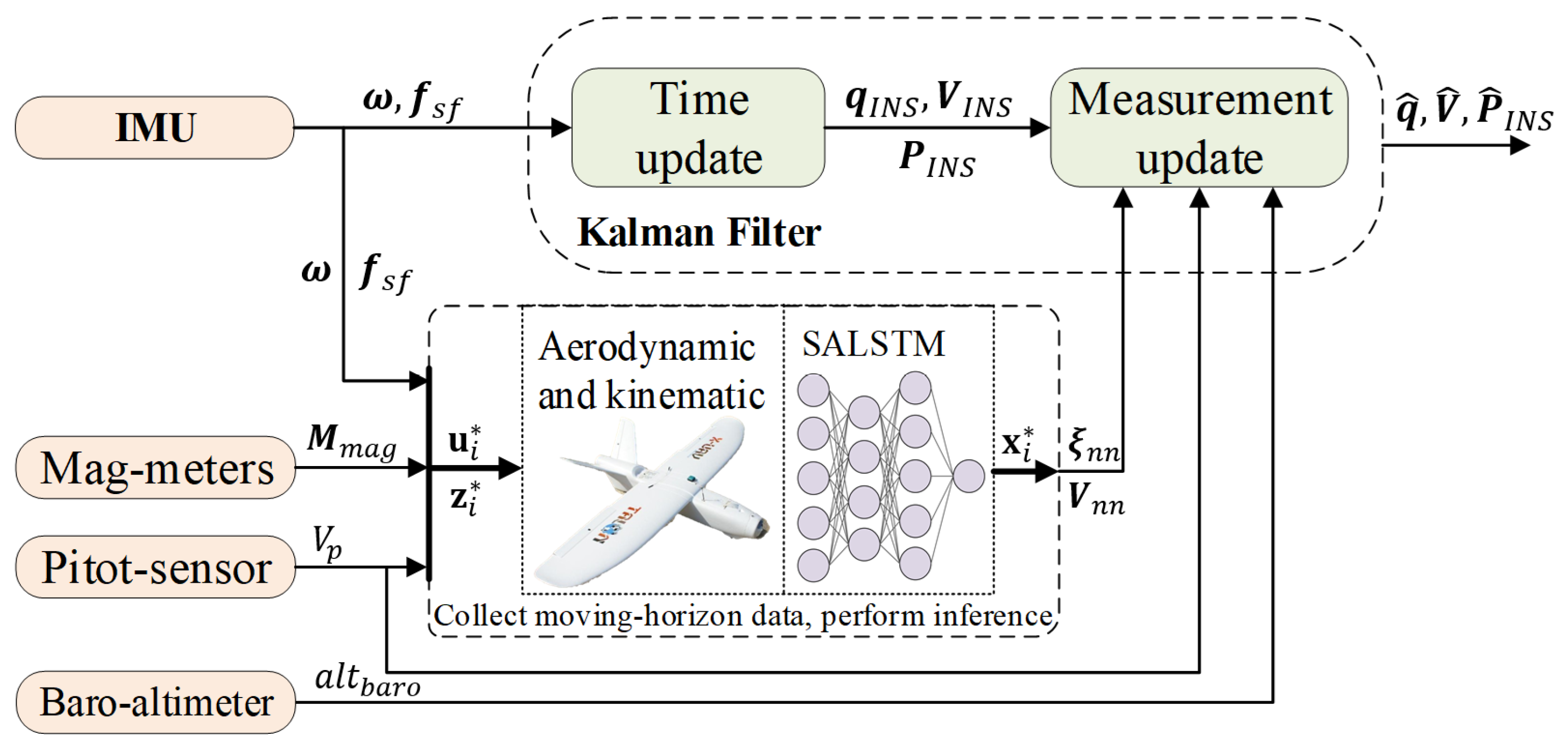
3.2. Data Fusing Methodology

The system model of UAVs is vital in capturing the dynamic of UAV maneuvers in integrated navigation. Considering the nonlinearity of kinematics in the flight environment, a nonlinear system model is used, which is assumed to satisfy the Gaussian process as follows:

$$\left\{\begin{array}{c}\begin{array}{l}{\mathbf{x}}_k=\mathbf{f}\left({\mathbf{x}}_{k-1},{\mathbf{u}}_{k-1}\right)+{\mathsf{\nu }}_{k-1}\\ {\mathbf{z}}_k^{\left(i\right)}={\mathbf{h}}^{\left(i\right)}\left({\mathbf{x}}_k,{\mathbf{u}}_k,\right)+{\mathsf{\eta }}_k^{\left(i\right)}\end{array}\end{array}\right.$$

(17)

where ${\mathbf{x}}_k$ is the system state; ${\mathbf{z}}_k^{\left(i\right)}$ is the measurement vector; $\mathbf{f}\left(·\right)$ and $\mathbf{h}\left(·\right)$ are the nonlinear system dynamic and measurement equation, respectively; ${\mathit{\nu }}_k$ and ${\mathsf{\eta }}_k^{\left(i\right)}$ are Gaussian observation white noise; and $i$ is the number of measurement equations of the system model.

The navigation strategies are carried out in the navigation frame. The state vector includes the unit quaternion, ground velocity, position, angular rate bias (${\mathit{b}}_{\omega }$), acceleration bias (${\mathit{b}}_f$), and two-dimensional horizontal wind speed. The unit quaternion is often used for the fast attitude solution and rigid-body transformation. The Euler attitude can be derived using a unit quaternion. The $\mathbf{x}$ vector is designed with a 19-dimensional state denoted by Equation (18).

$$\mathit{x}={\left[\begin{array}{c}\mathit{q},\mathit{V},\mathit{P},{\mathit{b}}_{\omega },{\mathit{b}}_f,{\mathit{V}}_w\end{array}\right]}^T$$

(18)

The input ($\mathbf{u}$) includes the angular velocity and specific force measured by the IMU as follows:

$$\mathbf{u}={\left[\mathit{\omega },{\mathit{f}}_{sf}\right]}^T$$

(19)

Measurements (${\mathbf{z}}^{\left(i\right)}$) of different sensors include the following:

(1) Altitude by barometer: ${\mathbf{z}}^{\left(1\right)}={alt}_{bora}$.

(2) Pitot airspeed: ${\mathbf{z}}^{\left(2\right)}=V_p$.

(3) Neural network inference of attitude and velocity: ${\mathbf{z}}^{\left(3\right)}=\left[\begin{array}{c}{\mathit{\xi }}_{nn}\\ {\mathit{V}}_{nn}\end{array}\right]$.

3.2.1. System Dynamic

The quaternion ($\mathit{q}$) consists of four elements, and $\mathit{q}=q_0+q_{1}i+q_{2}j+q_{3}k$, $\mathit{q}$ is updated as follows:

$${\mathit{q}}_k={\mathit{q}}_{k-1}\otimes \mathsf{\Delta }\mathit{q}$$

(20)

where ${\mathit{q}}_k$ and ${\mathit{q}}_{k-1}$ are unit quaternions at times $t_k$ and $t_{k-1}$, respectively. The $\otimes$ symbol denotes the multiplication rule for quaternions, and $\mathsf{\Delta }\mathit{q}$ is calculated as follows:

$$\mathsf{\Delta }\mathit{q}\approx \left[\begin{array}{c}1\\ \mathit{\omega }/2\end{array}\right]$$

(21)

$\mathit{\omega }$ is modeled by the following equation:

$$\mathit{\omega }=\tilde{\mathit{\omega }}-{\mathit{n}}_{\omega }-{\mathit{b}}_{\omega }$$

(22)

where $\tilde{\mathit{\omega }}$ is the measured angular rate and ${\mathit{n}}_{\omega }$ is gyroscope noise. ${\mathit{b}}_{\omega }$ is the gyroscope zero bias and is generally modeled as a first-order Markov process with zero-mean Gaussian noise as follows:

$${\mathit{b}}_{\omega ,k}={\mathit{b}}_{\omega ,k-1}exp{\displaystyle \frac{-T_s}{T_{\omega }}}+{\mathit{n}}_{{\mathit{b}}_{\omega ,k-1}}$$

(23)

where $T_{\omega }$ is the gyroscope correction time, and ${\mathit{n}}_{{\mathit{b}}_{\omega ,k-1}}$ denotes zero-mean Gaussian noise.

The velocity and position can be derived in the navigation frame by Equations (24) and (25), respectively.

$${\mathit{V}}_k={\mathit{V}}_{k-1}+{\displaystyle \frac{1}{2}}{C}_{b,k-1}^n{\mathit{f}}_{sf,k-1}{T}_s+\mathit{g}{T}_s$$

(24)

$${\mathit{P}}_k={\mathit{P}}_{k-1}+{\displaystyle \frac{1}{2}}\left({\mathit{V}}_k+{\mathit{V}}_{k-1}\right)T_s$$

(25)

where ${\mathit{V}}_k$ and ${\mathit{P}}_k$ are the velocity and position at time $t_k$, respectively; $C_{b,k-1}^n$ is the rotation matrix at time $t_{k-1}$; and ${\mathit{f}}_{sf,k}$ is the specific force at time $t_k$, obtained by the following equation:

$${\mathit{f}}_{sf,k}={\tilde{\mathit{f}}}_{sf,k}-{\mathit{n}}_f-{\mathit{b}}_{f,k-1}$$

(26)

where ${\tilde{\mathit{f}}}_{sf,k}$ is the three-axis measured specific force and ${\mathit{n}}_f$ is accelerometer noise. ${\mathit{b}}_{f,k-1}$ is the accelerometer zero bias and is assumed to be a first-order Markov process with zero-mean Gaussian noise as follows:

$${\mathit{b}}_{f_k}={\mathit{b}}_{f_{k-1}}exp{\displaystyle \frac{-T_s}{T_f}}+{\mathit{n}}_{{\mathit{b}}_{f,k-1}}$$

(27)

where $T_f$ is the accelerometer correction time and ${\mathit{n}}_{{\mathit{b}}_{f,k-1}}$ is zero-mean Gaussian noise.

The 3D wind speed (${\mathit{V}}_{w,k}$) is updated according to the Dryden wind model [34] as follows:

$${\mathit{V}}_{w,k}={\mathit{V}}_{w,k-1}-T_s{V}_{a,k-1}\left({\mathit{V}}_{w,k-1}\circ {\displaystyle \frac{1}{{\mathit{L}}_{k-1}}}\right)+{\mathit{n}}_{V_{w,k}}$$

(28)

where ${\mathit{L}}_{k-1}$ is the spatial wavelength, “$\circ$” denotes the Hadamard product, and ${\mathit{n}}_{V_{w,k}}$ is the process noise:

$${\mathit{n}}_{V_{w,k}}={\mathit{\sigma }}_{{\mathit{V}}_w}\circ \sqrt{2T_s{V}_a/{\mathit{L}}_{k-1}}\circ {\mathit{\nu }}_{V_w}$$

(29)

where ${\mathit{\sigma }}_{V_w}$ is the noise amplitude and ${\mathit{\nu }}_{V_w}$ represents Gaussian white noise.

3.2.2. Measurement Model

The frequencies of the measurements are different, and if all measurements are processed uniformly, the solution will diverge from the sparsity of the measurement matrix [35]. Thus, this paper employs a distributed fusion correction according to the sampling frequency of measurements. In this study, the measurements (${\tilde{\mathbf{z}}}_k^{\left(i\right)}$) for integrated navigation include the barometric altitude (${alt}_{baro}$), pitot airspeed ($V_p$), and the real-time outputs inferred by the neural network (${\mathit{\xi }}_{nn}$ and ${\mathit{V}}_{nn}$). The measurement equations for different measurements are listed as follows:

$${\tilde{\mathbf{z}}}_k^{\left(1\right)}={alt}_{baro}={\mathbf{h}}^{\left(1\right)}\left({\mathbf{x}}_k,{\mathbf{u}}_k\right)+{\mathsf{\eta }}_k^{\left(1\right)}$$

(30)

$${\tilde{\mathbf{z}}}_k^{\left(2\right)}=V_p={\mathbf{h}}^{\left(2\right)}\left({\mathbf{x}}_k,{\mathbf{u}}_k\right)+{\mathsf{\eta }}_k^{\left(2\right)}$$

(31)

$${\tilde{\mathbf{z}}}_k^{\left(3\right)}=\left[\begin{array}{c}{\mathit{\xi }}_{nn}\\ {\mathit{V}}_{nn}\end{array}\right]={\mathbf{h}}^{\left(3\right)}\left({\mathbf{x}}_k,{\mathbf{u}}_k\right)+{\mathsf{\eta }}_k^{\left(3\right)}$$

(32)

where ${\mathbf{h}}^{\left(i\right)}\left(·\right)$ represents the measurement equation of ${\tilde{\mathbf{z}}}_k^{\left(i\right)}$.

3.2.3. Implementation for EKF

In order to reduce the computational burden on the airborne navigation module while dealing with nonlinear dynamics, the EKF framework is used for fusion processing. For the navigation system using EKF, the process consists of time updates and measurement updates.

(1) Time update

The predicted state vector (${\widehat{\mathbf{x}}}_{k|k-1}$) is calculated using Equation (33), which is calculated based on the dynamic equations (Equations (20)–(29)).

$${\widehat{\mathbf{x}}}_{k|k-1}=F_{k|k-1}{\widehat{\mathbf{x}}}_{k-1|k-1}$$

(33)

where $F_{k|k-1}$ is the state transition matrix.

The predicted corresponding state covariance matrix (${\widehat{P}}_{k|k-1}$) can be obtained as follows:

$${\widehat{P}}_{k|k-1}=F_{k|k-1}{\widehat{P}}_{k-1|k-1}{F}_{k|k-1}^{\mathrm{T}}+Q_{k-1|k-1}$$

(34)

where $Q_{k-1|k-1}$ is the process covariance matrix.

(2) Measurement update

The sample frequencies of the mounted sensor of small fixed-wing UAVs are shown in Section 4.1. When either measurement is updated, the filter operates according to Equations (35)–(37).

The filtering gain is calculated as follows:

$$K_{k|k-1}^{\left(i\right)}={\widehat{P}}_{k|k-1}{H}_{k|k-1}^{\left(i\right),\mathrm{T}}/\left(H_{k|k-1}^{\left(i\right)}{\widehat{P}}_{k|k-1}{H}_{k|k-1}^{\left(i\right),\mathrm{T}}+R^{\left(i\right)}\right)$$

(35)

where $H_{k|k-1}^{\left(i\right)}$ is the Jacobian matrix derived from the sensor’s measurement equations, $R^{\left(i\right)}$ is the sensor noise covariance matrix, and $i$ is the number of sensors.

The corrected state vector (${\widehat{\mathbf{x}}}_{k|k}^{\left(i\right)}$) and corrected covariance matrix (${\widehat{P}}_{k|k}^{\left(i\right)}$) are estimated as follows:

$${\widehat{\mathbf{x}}}_{k|k}^{\left(i\right)}={\widehat{\mathbf{x}}}_{k|k-1}+K_{k|k-1}^{\left(i\right)}({\mathbf{z}}_k^{\left(i\right)}-{\mathit{h}}^{\left(i\right)}({\mathbf{x}}_k\left)\right)$$

(36)

$${\widehat{P}}_{k|k}^{\left(i\right)}=(I-K_{k|k-1}^{\left(i\right)}{H}_{k|k-1}^{\left(i\right)}){\widehat{P}}_{k|k-1}$$

(37)

where $I$ represents the identity matrix.

In order to utilize the pseudo-measurements of SALSTM and other sensor information within the EKF framework, it is necessary to derive the Jacobian matrix for measurement update. For different measurements, ${\mathit{H}}_{k|k-1}^{\left(i\right)}$ is derived by the following equations.

The correlation between ${alt}_{baro}$ and ${\mathbf{x}}_k$ is explicitly evident, with its measurement matrix expressed as follows:

$$H_{k|k-1}^{\left(1\right)}=\mathsf{\partial }{\mathbf{h}}^{\left(1\right)}\left({\mathbf{x}}_k,{\mathbf{u}}_k\right)/\mathsf{\partial }{\mathbf{x}}_k=\left[\begin{array}{ccc}{\mathbf{0}}_{1\times 7}& \left[\begin{array}{ccc}0& 0& 1\end{array}\right]& {\mathbf{0}}_{1\times 9}\end{array}\right]$$

(38)

The pitot airspeed sensor measures the UAV’s velocity relative to the surrounding air. That is, the pitot airspeed ($V_p$) is related to both the ground velocity and wind field as follow:

$$H_{k|k-1}^{\left(2\right)}=\mathsf{\partial }{\mathbf{h}}^{\left(2\right)}\left({\mathbf{x}}_k,{\mathbf{u}}_k\right)/\mathsf{\partial }{\mathbf{x}}_k=\left[\begin{array}{cccc}{\mathbf{0}}_{1\times 4}& {\mathit{H}}_{\mathit{V},1\times 3}^{V_p}& {\mathbf{0}}_{1\times 9}& {\mathit{H}}_{{\mathit{V}}_w,1\times 3}^{V_p}\end{array}\right]$$

(39)

The pitot airspeed is generally insensitive to small flow angles. It is approximately equal to the magnitude of the relative velocity vector between the UAV and the surrounding air. According to the “wind triangle”, the observation equation for the pitot airspeed is expressed as follows:

$$V_p=‖{\mathit{V}}^n-{\mathit{V}}_w^n‖$$

(40)

Therefore,

$${\mathit{H}}_{\mathit{V}}^{V_p}=\mathsf{\partial }{V}_p/\mathsf{\partial }{\mathit{V}}^n=\left[\begin{array}{ccc}{\displaystyle \frac{V^N-V_w^N}{‖{\mathit{V}}^n-{\mathit{V}}_w^n‖}}& {\displaystyle \frac{V^E-V_w^E}{‖{\mathit{V}}^n-{\mathit{V}}_w^n‖}}& {\displaystyle \frac{V^D}{‖{\mathit{V}}^n-{\mathit{V}}_w^n‖}}\end{array}\right]$$

(41)

$${\mathit{H}}_{{\mathit{V}}_w}^{V_p}=\mathsf{\partial }{V}_p/\mathsf{\partial }{\mathit{V}}_w^n=-\left[\begin{array}{cc}{\displaystyle \frac{V^N-V_w^N}{‖{\mathit{V}}^n-{\mathit{V}}_w^n‖}}& {\displaystyle \frac{V^E-V_w^E}{‖{\mathit{V}}^n-{\mathit{V}}_w^n‖}}\end{array}\right]$$

(42)

where superscripts $N$, $E$, and $D$ represent the components of the variables in the NED navigation frame.

For attitude and velocity inferred by the neural network, The Jacobian matrix derived from measurement equations is expressed as follows:

$$H_{k|k-1}^{\left(3\right)}=\mathsf{\partial }{\mathbf{h}}^{\left(3\right)}\left({\mathbf{x}}_k,{\mathbf{u}}_k\right)/\mathsf{\partial }{\mathbf{x}}_k=\left[\begin{array}{c}\begin{array}{ccc}{\mathit{H}}_{\mathit{q},1\times 4}^{\varphi }& {\mathbf{0}}_{1\times 3}& {\mathbf{0}}_{1\times 11}\\ {\mathit{H}}_{\mathit{q},1\times 4}^{\theta }& {\mathbf{0}}_{1\times 3}& {\mathbf{0}}_{1\times 11}\\ {\mathit{H}}_{\mathit{q},1\times 4}^{\psi }& {\mathbf{0}}_{1\times 3}& {\mathbf{0}}_{1\times 11}\\ {\mathbf{0}}_{3\times 4}& {\mathit{I}}_{3\times 3}& {\mathbf{0}}_{3\times 11}\end{array}\end{array}\right]$$

(43)

where ${\mathit{H}}_{\mathit{q}}^{\varphi }$, ${\mathit{H}}_{\mathit{q}}^{\theta }$, and ${\mathit{H}}_{\mathit{q}}^{\psi }$ are derived in detail in Appendix A.

3.3. SALSTM Network Design

In this study, the neural network is used to map sequences ${\mathbf{z}}_i^{\mathbf{*}}$ and ${\mathbf{u}}_i^{*}$ to optimal ${\mathbf{x}}_i^{*}$ based on the collected data, thereby avoiding the need for online optimization and solving the objective function. Referring to the estimation model in Section 2, the values of ${\mathbf{z}}_i^{\mathbf{*}}$ and ${\mathbf{u}}_i^{*}$ are treated as the neural network’s input ($u_i$), which is used to infer the system state (${\mathbf{x}}_i^{*}$) as follows:

$$u_i=\left[\begin{array}{c}{\left[V_{p,i},M_i^x,M_i^y,M_i^z\right]}^T\\ {\mathit{\omega }}_i\\ {\mathit{f}}_{\mathit{s}\mathit{f},i}\end{array}\right]$$

(44)

$${\mathbf{x}}_i^{*}=\left[\begin{array}{c}{\mathit{\xi }}_i\\ {\mathit{V}}_i^n\end{array}\right]$$

(45)

The role of the neural network is to establish an optimal mapping during training, then use this mapping during deployment to infer the system state, approximating the optimal value.

3.3.1. SALSTM Architecture

We consider the attitude and velocity estimation problem described in Section 2 as a time-series regression task and design the SALSTM network architecture. The SALSTM architecture leverages LSTM units for their ability to capture temporal dependencies and self-attention for its strength in modeling contextual relationships.

Given that temporal continuity of motion states is a critical constraint in dynamic models of UAVs, LSTM components are incorporated into SALSTM instead of using a pure self-attention structure (transformer). By leveraging the recurrent structure of LSTM in both the input and output layers, we effectively capture and maintain strict temporal continuity. The primary reason for not adopting a more computationally efficient GRU network is to leverage LSTM’s cell state to propagate time-continuous states such as wind and magnetic fields.

As shown in Figure 5, SALSTM consists of four layers. Its objective is to learn a function that maps the input sequence $\left[{u_{k-n},\cdots u_{k-1},u}_k\right]$ to its corresponding output sequence $\left[{\mathbf{x}}_{k-m}^{*},\cdots {\mathbf{x}}_{k-1}^{*},{\mathbf{x}}_k^{*}\right]$ from the training set, where $n$ is the length of the input sequence and $m$ is the length of the output sequence. The input vector ($u_k\in \mathbb{R}10$), consisting of $\mathit{f}$, $\mathit{\omega }$, $V_p$, and ${\mathit{M}}_{mag}$, and the output (${\mathbf{x}}_k^{*}\in \mathbb{R}6$) include the collected ground-truth values ($\widehat{\mathit{\xi }}$ and $\widehat{\mathit{V}}$).

3.3.2. LSTM Component

LSTM units are RNNs capable of selectively recognizing long sequences, proposed to solve the vanishing gradient problem presented in older variants. A LSTM unit is based on three main gates—an input gate, forget gate, and output gate—in addition to a cell state [36]. A detailed illustration of an LSTM unit is presented in Figure 6. The input gate is charged with collecting information, the forget gate decides on the information to forget and store, and the output gate updates the unit value. These gates allow for the control of information flow in the unit. The LSTM unit can be computed by calculating the different gates. At instance $k$, the input gate is $i_k$, the forget gate is $l_k$, and the output gate is $o_k$. The presented gates can be computed as follows:

$$\left\{\begin{array}{c}{i}_k={\sigma }_g\left(w_i{x}_k+u_i{h}_{k-1}+b_i\right)\\ l_k={\sigma }_g\left(w_f{x}_k+u_f{h}_{k-1}+b_f\right)\\ o_k={\sigma }_g\left(w_o{x}_k+u_o{h}_{k-1}+b_o\right)\end{array}\right.$$

(46)

where $h_k$ is the hidden state; $c_k$ is the cell state $; w_{*}$, $u_{*}$, and $b_{*}$ are the network parameter matrices to be learned.

The LSTM units are applied in the first, second, and fourth layers. The first and second LSTM layers are used to extract the autocorrelation features within the input sequences. More importantly, the LSTM layers can determine the complex temporal dynamics of the UAV’s movement through the hidden state ($h_k$) and cell state ($c_k$). The recursive nature of the LSTM layer effectively models the dynamic properties (Equation (8)). Cells within a single LSTM layer share the same structure and parameters, which are thought to reflect the time-invariant dynamic parameters (${\mathbf{p}}^{*}$) of the UAV. The use of a two-layer stacked LSTM structure enables better capture of the underlying features and complex dependencies.

The fourth LSTM layer serves as the output layer. Its primary function is to recover the recursive relationship within the output sequence $\left[{\mathbf{x}}_{k-m}^{*},\cdots {\mathbf{x}}_{k-1}^{*},{\mathbf{x}}_k^{*}\right]$ based on the weight connections within the self-attention layer. According to the state estimation model described in Section 2.4, the recursive poverty within outputs is modeled as time-continuous constraints. Therefore, we set the number of timesteps in the output layer to be $m$, where $m$ is selectable between 2 and $n$, that is, the output of the neural network during both training and inference is a sequence of length $m$, although only the final output (${\mathbf{x}}_k^{*}$) is fused in the EKF framework. In contrast, if the output is specified for a single timestep, learning the continuity constraints within the outputs becomes challenging.

3.3.3. Self-Attention Component

The self-attention layer is inserted as the third layer, with the primary objective of mitigating the vanishing gradient problem and extracting information from subtle dynamic changes of the UAV. Due to the recursive nature of the LSTM layer, the final output of an LSTM cell is more reliant on recent data. By introducing the self-attention mechanism, a shortcut connection is established between the output layer and all hidden states of the second LSTM layer. The weights of these shortcut connections can be adaptively adjusted for each hidden state, effectively preventing the inference from producing anomalous values.

In the SALSTM architecture, the data input to the third layer comprise the complete set of hidden states output from all units in the second LSTM layer, which fundamentally necessitates the incorporation of the self-attention mechanism. The self-attention mechanism processes three fundamental components—query (${\mathit{Q}}^{\mathit{*}}$), key (${\mathit{K}}^{\mathit{*}}$), and value ${\mathit{V}}^{\mathit{*}}$—ultimately producing a new sequence enriched with interactive information [37]. Given that ${\mathit{Q}}^{\mathit{*}}$ and ${\mathit{K}}^{\mathit{*}}$ share identical sequence lengths in SALSTM, the scaled dot-product attention mechanism is implemented to enhance computational efficiency, numerical stability, and representational capacity. The computational procedure of self-attention comprises four sequential operations: (1) computing the dot product between query and key matrices, (2) scaling the result by the square root of the dimension of keys ($d_k$), (3) applying the softmax function to generate the weight matrix, and (4) computing the final output through the dot product between the weight matrix and value matrix. The output is mathematically expressed as follows:

$$\mathit{i}\left({\mathit{Q}}^{\mathit{*}},{\mathit{K}}^{\mathit{*}},{\mathit{V}}^{\mathit{*}}\right)=\mathrm{S}\mathrm{o}\mathrm{f}\mathrm{t}\mathrm{m}\mathrm{a}\mathrm{x}\left({\displaystyle \frac{{\mathit{Q}}^{\mathit{*}}{{\mathit{K}}^{\mathit{*}}}^T}{\sqrt{d_k}}}\right)·{\mathit{V}}^{\mathit{*}}$$

(47)

where $\mathrm{S}\mathrm{o}\mathrm{f}\mathrm{t}\mathrm{m}\mathrm{a}\mathrm{x}\left({\mathit{A}}_i\right)={\mathrm{e}}^{{\mathit{A}}_i}/{\sum }_{j=k-n}^k{\mathrm{e}}^{{\mathit{A}}_j}$ and ${\mathit{A}}_i$ represents the i-th element of the input sequence.

4. Experimental Section

This section presents an evaluation of SALSTM-enhanced integrated navigation during an artificially induced GNSS outage. The evaluation is handled using two datasets, which were collected during field flight tests.

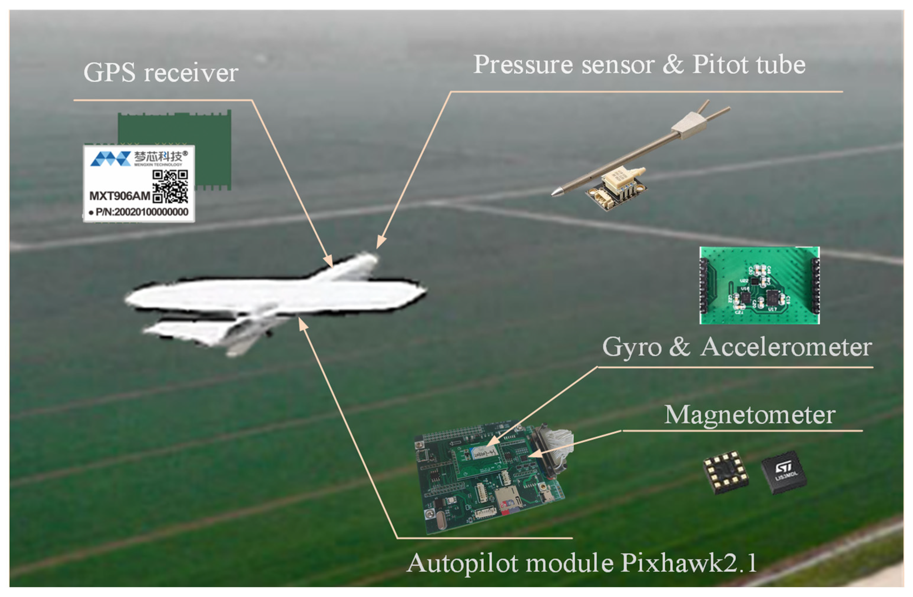
4.1. Hardware Configuration

The datasets used in this study were collected by Talon, a fixed-wing small UAV, as illustrated in Figure 7. Talon is equipped with a high-end BMI160 six-axis inertial measurement unit, an MXT906AM GPS receiver, a magnetometer, a barometer, and a pitot tube. The detailed parameters of these sensors are listed in

Table 1. Sensor performance parameters.

Sensor	Type	Noise/Error	Frequency
BMI160	Gyro Accelerometer	0.014°/S/√Hz	250 Hz
		150 µg/√Hz
MXT906AM	GPS receiver	pos: 2.5 m vel: 0.1 m/s	5 Hz
LIS3MDL	Magnetometer	3.2 mG	/
MS5611	Barometer	0.027 mbar	1024 Hz
MS5525	Pressure sensor & Pitot tube	0.84 Pa	100 Hz

. The raw data from these sensors are read and stored by a Pixhawk 2.1 hardware module within the PX 4 1.8.0 software framework.

In the PX4 software framework, the data of inertial sensors are fused with data from the GPS module, achieving a final accuracy of $0.8°$ in attitude, $0.1 \mathrm{m}/\mathrm{s}$ in velocity, and $2.5 \mathrm{m}$ in position [35,38]. These navigation states with GPS data fusion are also stored for SALSTM training or as reference for test.

4.2. Field Test Setup

In this study, two field flights were conducted using the Talon platform with the integrated navigation system under test. Complete sensor data were collected and stored for both flights. One of the flights provided 12 min of valid data, consisting of approximately 180,153 IMU data points, which were used to train and validate the SALSTM model. Talon performed various dynamically rich maneuvers during flight to ensure that collected data covered a broad spectrum of possible flight patterns, which is crucial for learning [1]. The data from the other flight contained 162,835 IMU data points over 11 min, which were used for an independent test of the method’s performance. These two field flight tests were conducted in Anhui Province, China, in a standard airplane flight field within legal airspace.

The steps were the same for both flight tests. Firstly, the structure and electrical components of Talon were checked. The UAV navigation states were initialized using the three-axis onboard accelerometer, gyroscope, and magnetometer, as well as the px4 autopilot initialization algorithm. Then, Talon took off remotely in “stabilized” mode and subsequently switched to “mission” mode to fly autonomously along the preset routes (shown in Figure 8). After switching to “mission” mode, flight data started to be recorded to ensure stable acquisition conditions and to guarantee the validity of the measurement data.

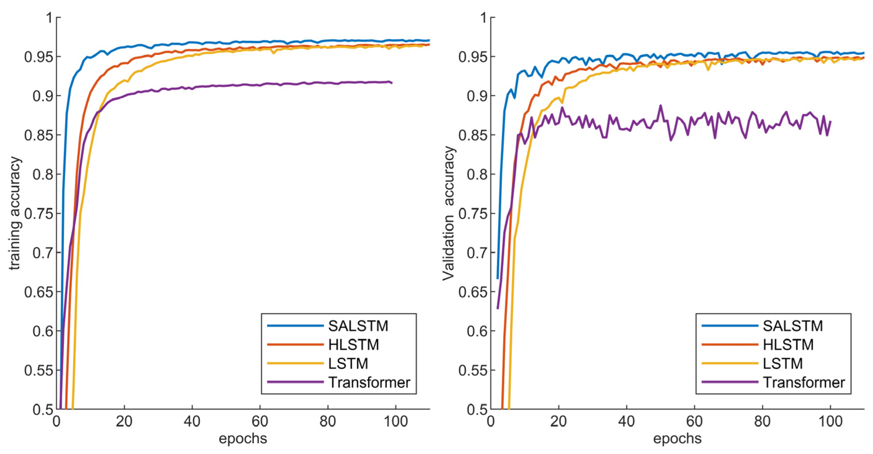
4.3. Model Pre-Training

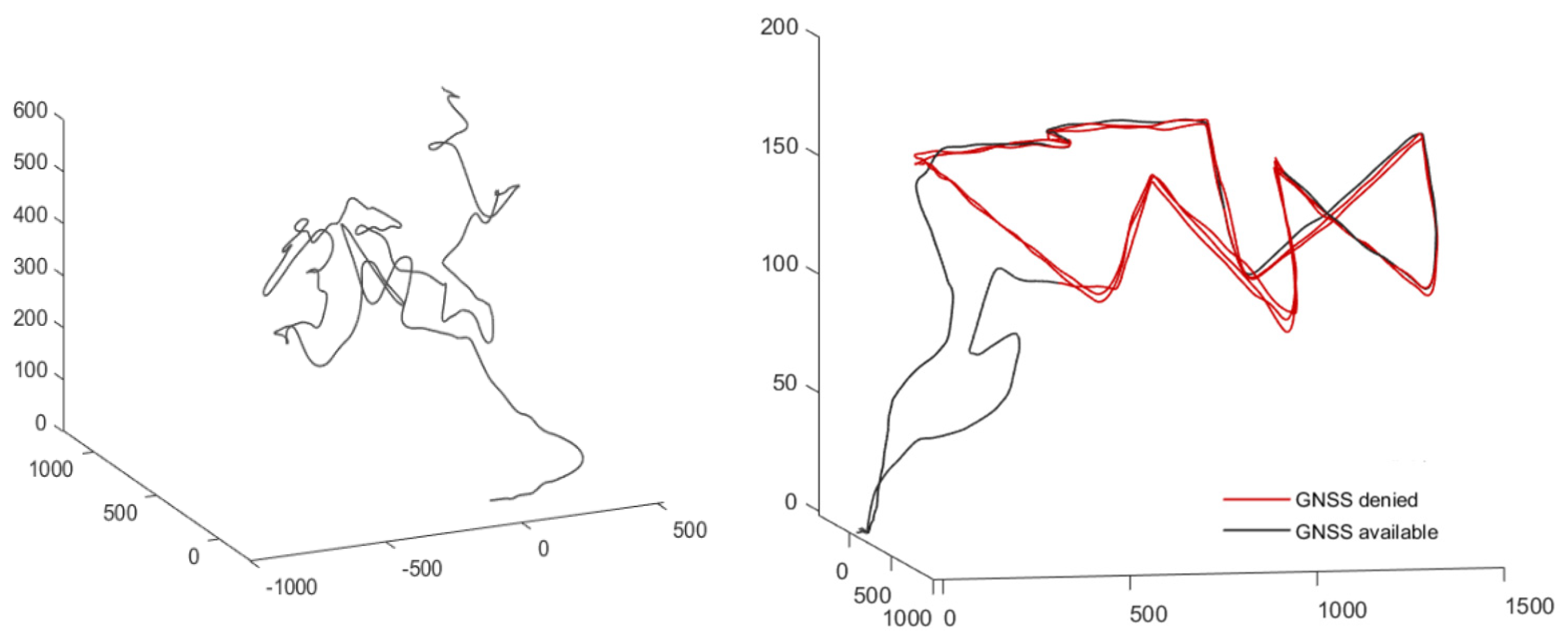
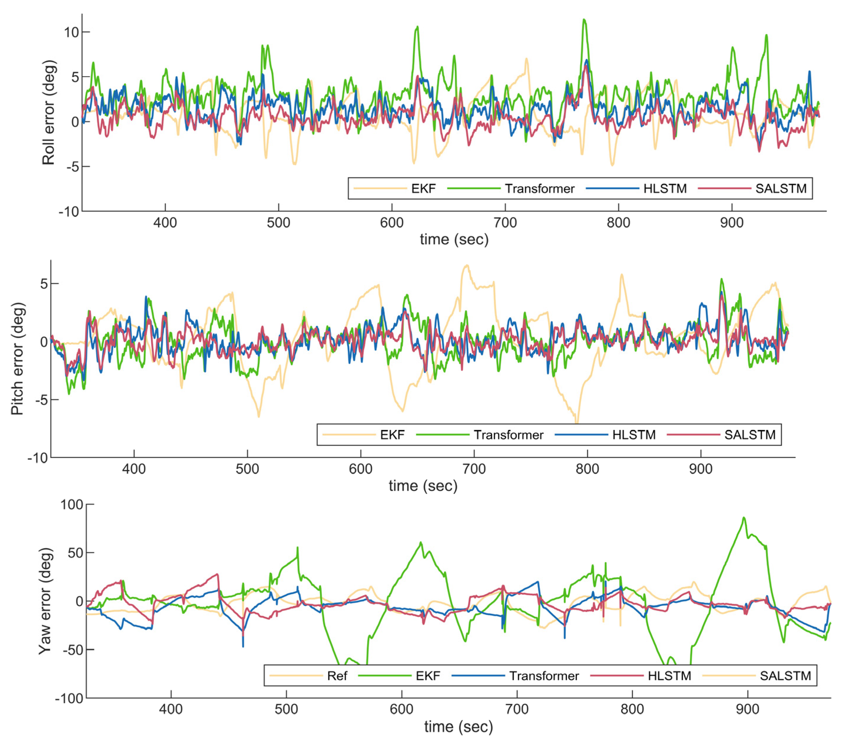
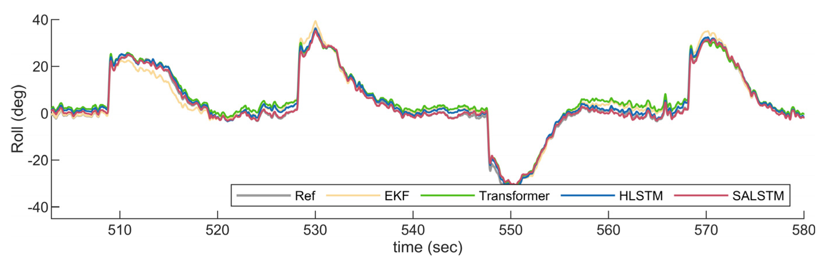
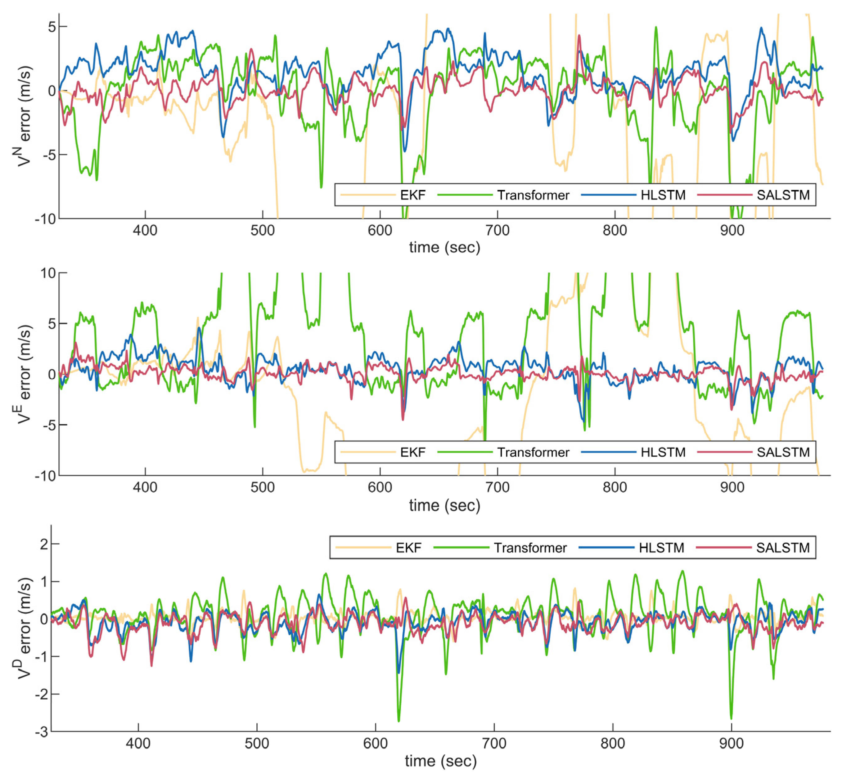
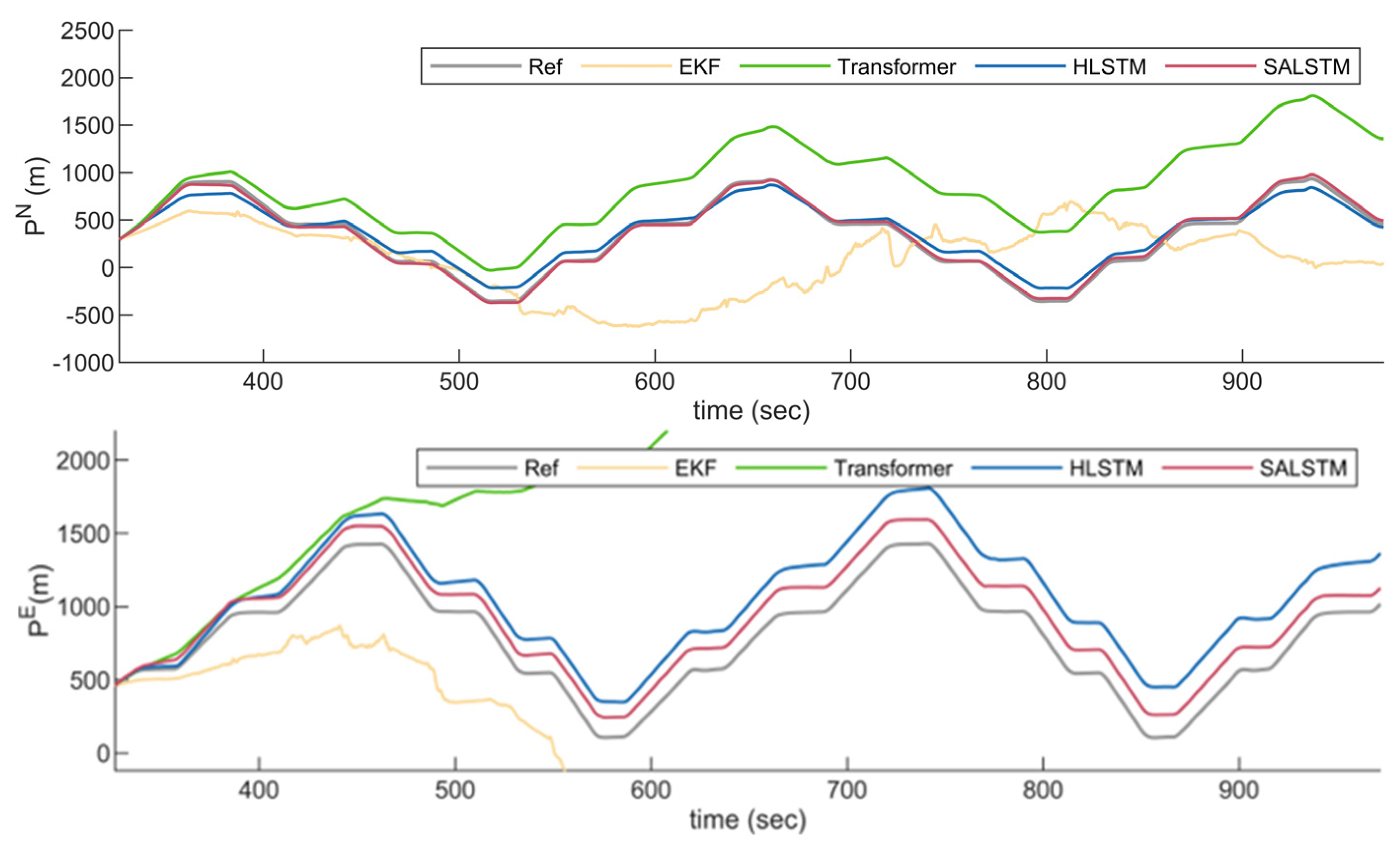
After the completion of the two flights, we performed the pre-training of the SALSTM model based on data of the first flight. To evaluate the performance of the proposed algorithm in GNSS-denied environments, we first compare SALSTM with the following methods: LSTM, hierarchical LSTM (HLSTM), and Transformer. These three comparison networks share the same input and output as SALSTM.

The collected data were interpolated based on time stamps to ensure temporal continuity, then downsampled to 50 Hz for efficient utilization. Min–max normalization was applied to both the input and output data of SALSTM across all dimensions. A 6:4 split ratio was applied to divide dataset 1 into training and validation sets with sizes of 19,557 and 13,039 samples, respectively. It should be noted that after deployment, the outputs of SALSTM were rescaled using the normalization parameters to revert to their original scales.

As indicated in

Table 2. Parameters of various models.

Model	Cost Function	Batch Size	Dropout	Learning Rate	Activation Function	Optimizer
Transformer	MSE	300	0.2	0.01	GELU, Softmax	Adam
LSTM, HLSTM	MSE	300	0.2	0.01	tanh, sigmoid	Adam
SALSTM	MSE	300	0.2	0.01	Softmax, tanh, sigmoid	Adam

, the mean square error (MSE) cost function, given by Equation (48), was chosen for learning. We utilized a regularization approach known as dropout to prevent the SALSTM model from overfitting. The initial learning rate was set to 0.01, with a decay factor of 0.7 and a minimum learning rate of ${10}^{-5}$. Each method’s training process was set to a maximum of 500 epochs, while early stopping was triggered if the loss function did not decrease significantly. The model parameters were empirically tuned to achieve the best feasible accuracy within the designed SALSTM architecture.

$$\mathrm{M}\mathrm{S}\mathrm{E}={\displaystyle \frac{1}{o}}\sum _{i=1}^o \sum _{j=k-m}^k |{\mathbf{x}}_j^{*}-y_j{|}^2$$

(48)

where ${\mathbf{x}}_j^{*}$ and $y_j$ denote the estimated and observed outputs and $o$ is the batch size when training is carried out.

Figure 9 depicts the accuracy achieved during the training procedure. The criterion evaluating the learning accuracy is defined as [1] $Accuracy=1-{\tan }^{-1}\mathrm{M}\mathrm{S}\mathrm{E}$. Compared with other networks, Figure 9 indicates that the SALSTM model adapts better to training data. In both training and validation data sets, SALSTM not only shows the highest learning efficiency but also achieves the highest accuracy. Compared to the Transformer model [30,31], SALSTM guarantees the time-continuous feature of the navigation state in both the input and output layers, while compared to the technique of simply stacking LSTM layers [19] and HLSTM [39], the self-attention layer inserted in the middle of SALSTM allows for the establishment of cross-time and cross-space connections of the measurement values, thereby avoiding gradient vanishing caused by measurement noise and long sequence learning.

Real-time performance is critical for navigation systems. The inference times of the four models are presented in

Table 3. Average inference times of various models (based on 10 trials).

Model	Transformer	LSTM	HLSTM	SALSTM
Total params	187,229	177,600	190,290	166,243
Inference time (s)	0.042	0.044	0.047	0.044

. These times are considered acceptable for two reasons. First, the navigation software incorporates a caching mechanism to handle measurement delays and ensure temporal alignment. Second, the SALSTM inference results are fused within the EKF framework, enabling the final navigation-state output to exceed 200 Hz.

The measurement errors are assumed to be independently distributed. The covariance of ${\mathit{\xi }}_{nn}$ and ${\mathit{V}}_{nn}$ is constructed based on the MSE of the SALSTM inference results obtained during training. The covariance of measurement vector (${\mathbf{z}}^{\left(3\right)}$) is set as follows:

$$R^{\left(3\right)}=\mathbf{d}\mathbf{i}\mathbf{a}\mathbf{g}\left({0.04}^2,{0.02}^2,{0.09}^2,{0.25}^2,{1.26}^2,{0.47}^2\right)$$

(49)

where the “$\mathbf{d}\mathbf{i}\mathbf{a}\mathbf{g}\left(a\right)$” stands for a diagonal matrix with $a$ on the main diagonal.

4.4. Test Results

To validate the proposed method, the model trained on dataset 1 in Section 4.3 was integrated into the integrated navigation framework described in Section 3.1. For comparison with three other methods, this study utilized the PX4 open-source offline navigation replay module (“PX4 replay”). This module employs the same navigation algorithm as the Talon airborne navigation module, except for the neural network inference fusion component. To avoid errors caused by overfitting, the sensor data used for replay were collected during the second flight (dataset 2). As for the reference true values, velocity and position were obtained from GNSS measurements, while attitude was derived from INS/GNSS fusion estimation results.

We selected HLSTM to represent the best performance of RNN-based networks and chose Transformer to represent the optimal performance of pure attention-based mechanisms. During the replay, at 326 s, GNSS signals were intentionally blocked by preconfiguring the PX4 replay’s parameters, while the pitot tube, INS, and barometer continued to operate normally. During this outage, the navigation system was aided by SALSTM, which provided $\left[{\varphi }_{nn},{\theta }_{nn},{\psi }_{nn},V_{nn}^N,V_{nn}^E,V_{nn}^D\right]$ as pseudo-measurements.

(1) Attitude and heading

In dataset 2, the Talon UAV executed multiple turns and pitch maneuvers. Throughout the 640 s GNSS outage, the roll angle exhibited fluctuations within the range of −30° to 30°, while the pitch angle varied between −10° and 20°. As shown in Figure 10, the three neural network-enhanced integrated navigation strategies demonstrated exceptional robustness, with no discernible cumulative errors in attitude estimation. Conversely, the EKF approach, devoid of neural network support, manifested pronounced cumulative errors in attitude estimation. Both the SALSTM and HLSTM methodologies achieved accurate heading estimation, in contrast to the Transformer method, which yielded suboptimal results. Notably, the standalone EKF was still capable of heading estimation due to the availability of the magnetometer.

Table 4. RMSE of attitude estimates of various methods during GNSS denial.

State	EKF	Transformer	HLSTM	SALSTM
Roll $\left(°\right)$	2.16	3.52	1.72	1.36
Pitch $\left(°\right)$	2.79	1.52	1.17	0.98
Yaw $\left(°\right)$	9.55	32.50	11.97	9.39

presents the statistical characteristics of the estimation performance for the three neural networks and the EKF framework.

Figure 11 illustrates the detailed performance of the roll-angle estimates. Compared to HLSTM and Transformer, the proposed SALSTM network achieved superior performance, particularly in roll-angle estimation. As shown in the figure, this advantage is primarily evident when the roll angle remains relatively small—a condition under which the dynamic characteristics of the UAV are less pronounced and more challenging to capture. The recursive nature of LSTM makes it prone to gradient vanishing, whereas the self-attention mechanism effectively captures these subtle dynamic changes. On the other hand, the Transformer model, which relies solely on the self-attention mechanism as its core component, also underperformed. Due to the absence of explicit recurrent architectures, Transformers face inherent limitations in preserving the temporal continuity required for dynamic systems modeling.

(2) Velocity

During the test, the Talon’s flight speed fluctuated between 15.9 and 23.3 m/s. Figure 12 depicts the velocity estimation results of various methods. The navigation system based on SALSTM continues to perform more accurately than other methods in long-term velocity estimation, followed by the LSTM and HALSTM networks, while the transformer model exhibits the poorest performance.

Table 5. RMSE of ground velocity estimates of various methods during GNSS denial.

State	EKF	Transformer	HLSTM	SALSTM
$V^N \left(\mathrm{m}/\mathrm{s}\right)$	20.05	3.04	2.14	1.02
$V^E \left(\mathrm{m}/\mathrm{s}\right)$	30.16	9.00	1.33	1.06
$V^D \left(\mathrm{m}/\mathrm{s}\right)$	0.17	0.53	0.28	0.27

presents the statistical characteristics of the velocity estimation performance for the three neural networks and the EKF.

Specifically, the diverging velocity estimates of the conventional EKF are attributed to the stand-alone INS calculations, which result in error accumulation. The Transformer model performs significantly better in estimating northward velocity than eastward velocity, a phenomenon that warrants further analysis. Nevertheless, the Transformer’s results remain unacceptable, with a root mean square error (RMSE) as high as 9 m/s. In contrast, the velocity estimations of HLSTM and SALSTM are considerably more accurate.

Compared to HLSTM, SALSTM achieves more precise estimation under conditions of slow speed variations (as shown in Figure 13). This is because in such scenarios, the dynamic characteristics of the UAV are difficult to excite. The self-attention layers integrated into the LSTM architecture effectively capture the subtle dynamic changes of the UAV.

(3) Position

Although the neural networks investigated in this study do not provide an inference value of position directly, the integrated navigation system can still achieve position estimation through velocity integration. The test data segment corresponds to a quadrilateral flight path, including multiple climbs and descents within a 1000 × 2000 × 100 m space.

As shown in Figure 14 and Figure 15, the position estimation results of the HLSTM and SALSTM methods remain stable, whereas the EKF and Transformer methods exhibit anomalous position estimates. Similarly, the SALSTM-enhanced integrated navigation system demonstrates the highest accuracy, with a horizontal position error of approximately 141 m. Considering the total flight duration of 640 s and a flight distance of 11,520 m, the achieved accuracy is remarkable, reaching 0.013. This is attributed to the measurements provided by SALSTM, which significantly reduce the NED velocity errors in the integrated navigation system, thereby substantially decreasing the cumulative position errors. Finally, due to the integration of barometer data, all methods achieve high-precision altitude estimation.

Table 6. RMSE of position estimates of various methods during GNSS denial.

State	EKF	Transformer	HLSTM	SALSTM
$P^N \left(\mathrm{m}\right)$	461.37	574.44	84.75	26.84
$P^E \left(\mathrm{m}\right)$	1477.98	2164.73	279.39	138.51
$P^{D }\left(\mathrm{m}\right)$	6.83	6.54	7.10	7.16

presents the statistical characteristics of the position estimation performance for the three neural networks and EKF.

Since there is no direct measurement available to correct the position in integrated navigation, the position error accumulates indefinitely over time. Therefore, the maximum accumulated position error after a continuous flight of 11 min is presented in

Table 7. Maximum position estimation error of various methods during GNSS denial.

State	EKF	Transformer	HLSTM	SALSTM
$P^{N }\left(\mathrm{m}\right)$	991.58	897.83	139.60	35.27
$P^E \left(\mathrm{m}\right)$	2525.42	3614.90	357.24	158.67

.

5. Conclusions and Discussion

Small fixed-wing UAVs equipped with MEMS-based inertial measurement units are prone to error accumulation during navigation in GNSS-denied environments. To address this issue, this study proposes a hybrid neural network, SALSTM, which combines self-attention mechanisms with LSTM to enhance integrated navigation performance. We first model the estimation task based on UAV aerodynamics and kinematics, which enables us to precisely define the inputs and outputs for SALSTM mapping. To improve performance when the UAV’s dynamics are not well-excited, a self-attention mechanism is incorporated into SALSTM to capture long-range dependencies in subtle dynamic changes. The self-attention layers are embedded within multiple LSTM layers, and the output layer is designed to generate state sequences, leveraging the recursive nature of LSTM to enforce state continuity constraints.

The real-time inference of attitude and velocity from SALSTM is fused into the EKF framework for integrated navigation. A distributed fusion framework is adopted to integrate multi-source measurements. To facilitate deployment on low-performance onboard hardware, we derive the Jacobian matrix of Euler attitude measurements.

The SALSTM-enhanced integrated navigation method is validated using data from two flight tests. Dataset 1 is used for training and validation, while dataset 2 serves for an independent test. The results demonstrate that the SALSTM-enhanced integrated navigation system achieves superior long-term stability, delivering consistent attitude and velocity estimation over extended periods while significantly improving position estimation accuracy. Over a 640 s duration, the root mean square errors for attitude and velocity are 1.36° and 1.06 m/s, respectively, with a total cumulative position error of approximately 162 m, representing 0.013 of the total flight distances. This represents a 50% improvement over the best existing methods.

Currently, the modeling approach treats wind field parameters as unknown constants due to the lack of real-time wind field measurements in this study. If future studies incorporate measurement tools to collect real-time wind field data, the trained model could also be applied to wind field estimation. Nevertheless, when wind field and geomagnetic parameters change, SALSTM requires online training using local flight data to adjust network parameters. Based on the modeling and analysis performed in this study, the SALSTM-enhanced navigation method is applicable to various fixed-wing UAVs. However, the current approach is not suitable for rotorcraft UAVs due to their distinct flight dynamics models. Additionally, further research is needed to investigate SALSTM’s noise modeling and the accuracy of its outputs under different sensor configurations. Moreover, the method’s generalization capability in scenarios not covered by the training data requires validation, particularly in high-maneuverability and near-stall flight conditions. We recommend collecting targeted flight data for training in these specific scenarios.

References

1. Taghizadeh, S.; Safabakhsh, R. An Integrated INS/GNSS System with an Attention-Based Hierarchical LSTM during GNSS Outage. GPS Solut. 2023, 27, 71. [Google Scholar] [CrossRef]
2. Daneshmand, S.; Lachapelle, G. Integration of GNSS and INS with a Phased Array Antenna. GPS Solut. 2018, 22, 3. [Google Scholar] [CrossRef]
3. Li, M.; Hu, T. Deep Learning Enabled Localization for UAV Autolanding. Chin. J. Aeronaut. 2021, 34, 585–600. [Google Scholar] [CrossRef]
4. Pasqualetto Cassinis, L.; Fonod, R.; Gill, E.; Ahrns, I.; Gil-Fernández, J. Evaluation of Tightly- and Loosely-Coupled Approaches in CNN-Based Pose Estimation Systems for Uncooperative Spacecraft. Acta Astronaut. 2021, 182, 189–202. [Google Scholar] [CrossRef]
5. Huang, H.; Yang, Y.; Wang, H.; Ding, Z.; Sari, H.; Adachi, F. Deep Reinforcement Learning for UAV Navigation Through Massive MIMO Technique. IEEE Trans. Veh. Technol. 2020, 69, 1117–1121. [Google Scholar] [CrossRef]
6. Lin, H.-Y.; Zhan, J.-R. GNSS-Denied UAV Indoor Navigation with UWB Incorporated Visual Inertial Odometry. Measurement 2023, 206, 112256. [Google Scholar] [CrossRef]
7. Liu, H.; Pan, S.; Wu, P.; Yu, K.; Gao, W.; Yu, B. Uncertainty-Aware UWB/LiDAR/INS Tightly Coupled Fusion Pose Estimation via Filtering Approach. IEEE Sens. J. 2024, 24, 11113–11126. [Google Scholar] [CrossRef]
8. He, G.; Yuan, X.; Zhuang, Y.; Hu, H. An Integrated GNSS/LiDAR-SLAM Pose Estimation Framework for Large-Scale Map Building in Partially GNSS-Denied Environments. IEEE Trans. Instrum. Meas. 2021, 70, 1–9. [Google Scholar] [CrossRef]
9. Guangcai, W.; Xu, X.; Zhang, T. M-M Estimation-Based Robust Cubature Kalman Filter for INS/GPS Integrated Navigation System. IEEE Trans. Instrum. Meas. 2021, 70, 1–11. [Google Scholar] [CrossRef]
10. Sabatini, R.; Roy, A.; Blasch, E.; Kramer, K.A.; Fasano, G.; Majid, I.; Crespillo, O.G.; Brown, D.A.; Ogan Major, R. Avionics Systems Panel Research and Innovation Perspectives. IEEE Aerosp. Electron. Syst. Mag. 2020, 35, 58–72. [Google Scholar] [CrossRef]
11. Sharaf, R.; Noureldin, A.; Osman, A.; El-Sheimy, N. Online INS/GPS Integration with a Radial Basis Function Neural Network. IEEE Aerosp. Electron. Syst. Mag. 2005, 20, 8–14. [Google Scholar]
12. Chen, L.; Fang, J. A Hybrid Prediction Method for Bridging GPS Outages in High-Precision POS Application. IEEE Trans. Instrum. Meas. 2014, 63, 1656–1665. [Google Scholar] [CrossRef]
13. Yao, Y.; Xu, X.; Zhu, C.; Chan, C.-Y. A Hybrid Fusion Algorithm for GPS/INS Integration during GPS Outages. Measurement 2017, 103, 42–51. [Google Scholar]
14. Taghizadeh, S.; Safabakhsh, R. An Integrated INS/GNSS System With an Attention-Based Deep Network for Drones in GNSS Denied Environments. IEEE Aerosp. Electron. Syst. Mag. 2023, 38, 14–25. [Google Scholar]
15. Malleswaran, M.; Vaidehi, V.; Sivasankari, N. A Novel Approach to the Integration of GPS and INS Using Recurrent Neural Networks with Evolutionary Optimization Techniques. Aerosp. Sci. Technol. 2014, 32, 169–179. [Google Scholar] [CrossRef]
16. Dai, H.; Bian, H.; Wang, R.; Ma, H. An INS/GNSS Integrated Navigation in GNSS Denied Environment Using Recurrent Neural Network. Def. Technol. 2020, 16, 334–340. [Google Scholar] [CrossRef]
17. Doostdar, P.; Keighobadi, J.; Hamed, M.A. INS/GNSS Integration Using Recurrent Fuzzy Wavelet Neural Networks. GPS Solut. 2020, 24, 29. [Google Scholar] [CrossRef]
18. Bijjahalli, S.; Sabatini, R.; Gardi, A. Advances in Intelligent and Autonomous Navigation Systems for Small UAS. Prog. Aerosp. Sci. 2020, 115, 100617. [Google Scholar]
19. Fang, W.; Jiang, J.; Lu, S.; Gong, Y.; Tao, Y.; Tang, Y.; Yan, P.; Luo, H.; Liu, J. A LSTM Algorithm Estimating Pseudo Measurements for Aiding INS during GNSS Signal Outages. Remote Sens. 2020, 12, 256. [Google Scholar] [CrossRef]
20. Zhang, Z.; Li, Y.; Liu, Z.; Wang, S.; Xing, H.; Zhu, W. Enhancing the Reliability of Shipborne INS/GNSS Integrated Navigation System during Abnormal Sampling Periods Using Bi-LSTM and Robust CKF. Ocean Eng. 2023, 288, 115934. [Google Scholar] [CrossRef]
21. Chen, S.; Xin, M.; Yang, F.; Zhang, X.; Liu, J.; Ren, G.; Kong, S. Error Compensation Method of GNSS/INS Integrated Navigation System Based on AT-LSTM during GNSS Outages. IEEE Sens. J. 2024, 24, 20188–20199. [Google Scholar]
22. Lv, P.-F.; Lv, J.-Y.; Hong, Z.-C.; Xu, L.-X. Integration of Deep Sequence Learning-Based Virtual GPS Model and EKF for AUV Navigation. Drones 2024, 8, 441. [Google Scholar] [CrossRef]
23. Chung, J.; Gulcehre, C.; Cho, K.; Bengio, Y. Empirical Evaluation of Gated Recurrent Neural Networks on Sequence Modeling 2014. arXiv 2014, arXiv:1412.3555. [Google Scholar]
24. Tang, Y.; Jiang, J.; Liu, J.; Yan, P.; Tao, Y.; Liu, J. A GRU and AKF-Based Hybrid Algorithm for Improving INS/GNSS Navigation Accuracy during GNSS Outage. Remote Sensing 2022, 14, 752. [Google Scholar]
25. Zhao, S.; Zhou, Y.; Huang, T. A Novel Method for AI-Assisted INS/GNSS Navigation System Based on CNN-GRU and CKF during GNSS Outage. Remote Sensing 2022, 14, 4494. [Google Scholar]
26. Meng, X.; Tan, H.; Yan, P.; Zheng, Q.; Chen, G.; Jiang, J. A GNSS/INS Integrated Navigation Compensation Method Based on CNN–GRU + IRAKF Hybrid Model During GNSS Outages. IEEE Trans. Instrum. Meas. 2024, 73, 1–15. [Google Scholar]
27. Guo, T.; Jiang, N.; Li, B.; Zhu, X.; Wang, Y.; Du, W. UAV Navigation in High Dynamic Environments: A Deep Reinforcement Learning Approach. Chin. J. Aeronaut. 2021, 34, 479–489. [Google Scholar]
28. Wu, Z.; Yao, Z.; Lu, M. Deep-Reinforcement-Learning-Based Autonomous Establishment of Local Positioning Systems in Unknown Indoor Environments. IEEE Internet Things J. 2022, 9, 13626–13637. [Google Scholar]
29. Xue, Y.; Chen, W. Multi-Agent Deep Reinforcement Learning for UAVs Navigation in Unknown Complex Environment. IEEE Trans. Intell. Veh. 2023, 9, 2290–2303. [Google Scholar]
30. Cheng, J.; Dong, L.; Lapata, M. Long Short-Term Memory-Networks for Machine Reading. arXiv 2016, arXiv:1601.06733. [Google Scholar]
31. Vaswani, A.; Shazeer, N.; Parmar, N.; Uszkoreit, J.; Jones, L.; Gomez, A.N.; Kaiser, Ł.; Polosukhin, I. Attention Is All You Need. In Proceedings of the 31st Conference on Neural Information Processing Systems (NIPS 2017), Long Beach, CA, USA, 4–9 December 2017. [Google Scholar]
32. Wang, Z.; Li, J.; Liu, C.; Yang, Y.; Li, J.; Wu, X.; Yang, Y.; Ye, B. Optimization-Assisted Filter for Flow Angle Estimation of SUAV Without Adequate Measurement. Drones 2024, 8, 758. [Google Scholar] [CrossRef]
33. Hu, G.; Wang, W.; Zhong, Y.; Gao, B.; Gu, C. A New Direct Filtering Approach to INS/GNSS Integration. Aerosp. Sci. Technol. 2018, 77, 755–764. [Google Scholar]
34. Cho, A.; Kim, J.; Lee, S.; Kee, C. Wind Estimation and Airspeed Calibration Using a UAV with a Single-Antenna GPS Receiver and Pitot Tube. IEEE Trans. Aerosp. Electron. Syst. 2011, 47, 109–117. [Google Scholar]
35. Yang, Y.; Liu, X.; Liu, X.; Guo, Y.; Zhang, W. Model-Free Integrated Navigation of Small Fixed-Wing UAVs Full State Estimation in Wind Disturbance. IEEE Sens. J. 2022, 22, 2771–2781. [Google Scholar]
36. Hochreiter, S.; Schmidhuber, J. Long Short-Term Memory. Neural Comput. 1997, 9, 1735–1780. [Google Scholar]
37. Jiang, W.; Cai, T.; Xu, G.; Wang, Y. Autonomous Obstacle Avoidance and Target Tracking of UAV: Transformer for Observation Sequence in Reinforcement Learning. Knowl.-Based Syst. 2024, 290, 111604. [Google Scholar]
38. Zhuang, Y.; Sun, X.; Li, Y.; Huai, J.; Hua, L.; Yang, X.; Cao, X.; Zhang, P.; Cao, Y.; Qi, L.; et al. Multi-Sensor Integrated Navigation/Positioning Systems Using Data Fusion: From Analytics-Based to Learning-Based Approaches. Inf. Fusion 2023, 95, 62–90. [Google Scholar]
39. Gandhi, A.; Sharma, A.; Biswas, A.; Deshmukh, O. GeThR-Net: A Generalized Temporally Hybrid Recurrent Neural Network for Multimodal Information Fusion. In Computer Vision–ECCV 2016 Workshops: Amsterdam, The Netherlands, October 8-10 and 15-16, 2016, Proceedings, Part II 14; Hua, G., Jégou, H., Eds.; Lecture Notes in Computer Science; Springer International Publishing: Cham, Switzerland, 2016; Volume 9914, pp. 883–899. ISBN 978-3-319-48880-6. [Google Scholar]
Figure 1. Research workflow for GNSS-denied navigation.
Drones 09 00279 g001
Figure 2. The involved coordinate system: wind frame, body frame, and navigation frame. The body frame is denoted as “ x b y b z b ” (front–right–down), and the navigation frame is denoted as “NED” (north–east–down). D , Y , and L are the drag, lateral, and lift forces.
Drones 09 00279 g002
Figure 3. Integrated navigation method (no background) and neural network training framework (gray background). The outputs of the integrated navigation system include position ( P ^ ), velocity ( V ^ ), and quaternion ( q ^ ). The ξ ^ values used for training are converted from q ^ .
Drones 09 00279 g003
Figure 4. SALSTM-enhanced integrated navigation framework in a GNSS-denied environment.
Drones 09 00279 g004
Figure 5. SALSTM architecture, which consists of four layers with a self-attention layer inserted in three LSTM layers. In this study, the parameter n is set to 72, and m is set to 10.
Drones 09 00279 g005
Figure 6. LSTM component.
Drones 09 00279 g006
Figure 7. Fixed-wing UAV Talon used for field tests. (Mass of Talon: 5.6 kg; cruise speed: 18 m/s).
Drones 09 00279 g007
Figure 8. The flight path for data collection. Dataset 1 was used for training (left), and dataset 2 was used for an independent test (right). The red-marked segment represents the valid data used for testing.
Drones 09 00279 g008
Figure 9. Accuracy performance of SALSTM. Training set (left) and validation set (right).
Drones 09 00279 g009
Figure 10. The Euler attitude error of the estimates. EKF (yellow), Transformer (green), HLSTM (blue), and SALSTM (red).
Drones 09 00279 g010
Figure 11. Details of the estimated roll attitude results for different schemes.
Drones 09 00279 g011
Figure 12. The velocity error of the estimates. EKF (yellow), Transformer (green), HLSTM (blue), and SALSTM (red).
Drones 09 00279 g012
Figure 13. NED velocity estimation performance. Ref (gray), Transformer (green), HLSTM (blue), and SALSTM (red).
Drones 09 00279 g013
Figure 14. The position error of the estimates. EKF (yellow), Transformer (green), HLSTM (blue), and SALSTM (red).
Drones 09 00279 g014
Figure 15. Position estimation performance. Ref (gray), EKF (yellow), Transformer (green), HLSTM (blue), and SALSTM (red).
Drones 09 00279 g015