Research on the Inversion Method of Dust Content on Mining Area Plant Canopies Based on UAV-Borne VNIR Hyperspectral Data

Abstract

Monitoring dust on plant canopies around open-pit coal mines is crucial to assessing environmental pollution and developing effective dust suppression strategies. This research focuses on the Ha’erwusu open-pit coal mine in Inner Mongolia, China, using measured dust content on plant canopies and UAV-borne VNIR hyperspectral data as the data sources. The study employed five spectral transformation forms—first derivative (FD), second derivative (SD), logarithm transformation (LT), reciprocal transformation (RT), and square root (SR)—alongside the competitive adaptive reweighted sampling (CARS) method to extract characteristic bands associated with canopy dust. Various regression models, including extreme learning machine (ELM), random forest (RF), partial least squares regression (PLSR), and support vector machine (SVM), were utilized to establish dust inversion models. The spatial distribution of canopy dust was then analyzed. The results demonstrate that the geometric and radiometric correction of the UAV-borne VNIR hyperspectral images successfully restored the true spatial information and spectral features. The spectral transformations significantly enhance the feature information for canopy dust. The CARS algorithm extracted characteristic bands representing 20 to 30% of the total spectral bands, evenly spread across the entire range, thereby reducing the estimation model’s computational complexity. Both feature extraction and model selection influence the inversion accuracy, with the LT-CARS and RF combination offering the best predictive performance. Canopy dust content decreases with increasing distance from the dust source. These findings offer valuable insights for canopy dust retention monitoring and offer a solid foundation for dust pollution management and the development of suppression strategies.

1. Introduction

Coal mining, as an essential energy industry component, has significantly contributed to economic development. The extraction of coal not only provides abundant energy resources but also directly promotes the infrastructure development, employment opportunities, and economic growth of mining areas and their surrounding regions [1,2]. However, during the coal mining process, especially in the extraction and transportation stages, the emission of large amounts of coal dust and delicate particulate matter has become a serious environmental issue [3,4]. The dispersion and deposition of dust are key factors affecting the ecological environment, as they damage the physicochemical properties of soil [5,6], inhibit plant photosynthesis and respiration [7,8,9], and pose potential threats to human health [10,11]. Plants, especially trees and shrubs, have a natural dust retention capacity, enabling them to absorb airborne particles [12]. This process is primarily facilitated by the leaf surface, stomata, and canopy structure. The rough surface and waxy coating of the leaves effectively capture dust, while the epidermal structure aids in particle adhesion. Stomata not only absorb carbon dioxide but also capture dust particles, directing them to the leaf surface through transpiration. Additionally, the dense foliage of the canopy obstructs airflow, promoting the deposition of dust particles onto the leaves. Plant dust retention is strongly influenced by factors like leaf area, leaf morphology, canopy structure, as well as environmental conditions and climate change [13]. Therefore, monitoring the canopy dust content not only helps assess the extent of dust pollution caused by coal mining and other industrial activities but also provides scientific support for ecological protection and pollution control.

To estimate canopy dust content with high accuracy, hyperspectral remote sensing has been increasingly used in recent years, offering both time- and labor-efficiency [14,15,16,17]. Currently, research on using spectral technology to monitor plant dust content mainly focuses on two aspects: analyzing the spectral response characteristics of dust retention and constructing quantitative inversion models [18,19,20]. Zhu et al. [21] utilized an ASD FieldSpec 3 spectrometer to collect hyperspectral data and investigate how dust retention affects leaf spectral properties. They developed a model for estimating dust content on leaf surfaces using hyperspectral data. Su et al. [22] studied the spectral response of leaf surfaces at varying levels of dust accumulation and used an inversion model with Sentinel-2 images to map the dust content distribution in evergreen vegetation. Jing et al. [23] used three common plant species from southern China as research objects, measured leaf spectra using the ASD FieldSpec 3, and constructed dust content inversion models based on three machine learning methods. Yan et al. [24] examined the spectral variations between dusty and clean leaves, investigated the relationship between dust accumulation and reflectance, and utilized MODIS images to derive dustfall distribution maps for Beijing. Wang et al. [25] investigated the correlation between the reflectance ratio (Dust/Clean) and dustfall weight, developing a regression model for dustfall weight using satellite band reflectance and NDVI. Wang et al. [26] examined the influence of dust on spectral reflectance and identified spectral bands most sensitive to dust, establishing a regression model for vegetation index ratio and dust content in satellite bands. Luo et al. [16] studied the effect of dust on leaf-scale plant spectral characteristics based on the spectral reflectance curves and partial least squares regression. Peng et al. [27] analyzed how foliar dustfall content (FDC) affects pear leaf hyperspectral properties and developed a quantitative model to invert FDC based on reflectance data.

Although the dust content inversion methods constructed using the ASD spectrometer (ASD Inc., Boulder, CO, USA) and satellite hyperspectral images have achieved good results, the coefficient of determination (R²) of the prediction model developed by Zhu et al. [28] exceeded 0.8, while Peng et al.’s [17] model achieved an impressive R² of 0.92. The ASD spectrometer can only capture point-source data, which limits its application in large-scale dust monitoring. Due to satellite images’ relatively low resolution, they are prone to the influence of mixed pixels, thereby limiting the accuracy of plant dust content monitoring. In contrast, UAV-borne VNIR hyperspectral data, with their high spatial resolution and short revisit cycle, offer a new solution that can efficiently and accurately monitor plant dust content in medium to small areas. Although the potential of UAV-borne VNIR hyperspectral data for plant dust content monitoring is gradually being recognized, research that combines characteristic band selection and machine learning algorithms for canopy dust content monitoring in mining areas is still relatively scarce.

This study focused on the Ha’erwusu open-pit coal mine in Inner Mongolia, China. Utilizing UAV-borne VNIR hyperspectral data and measured canopy dust content, various spectral transformations—including first derivative (FD), second derivative (SD), logarithmic transformation (LT), reciprocal transformation (RT), and square root transformation (SR)—were applied. Additionally, the competitive adaptive reweighted sampling (CARS) methods was used to extract characteristic bands. Inversion models for canopy dust content were developed by combining extreme learning machine (ELM), random forest (RF), partial least squares regression (PLSR), and support vector machine (SVM) algorithms. Based on the optimal model, spatial distribution maps of canopy dust content were derived, allowing for an analysis of the distribution characteristics. The results provide an essential reference for formulating effective dust control measures.

2. Materials and Methods

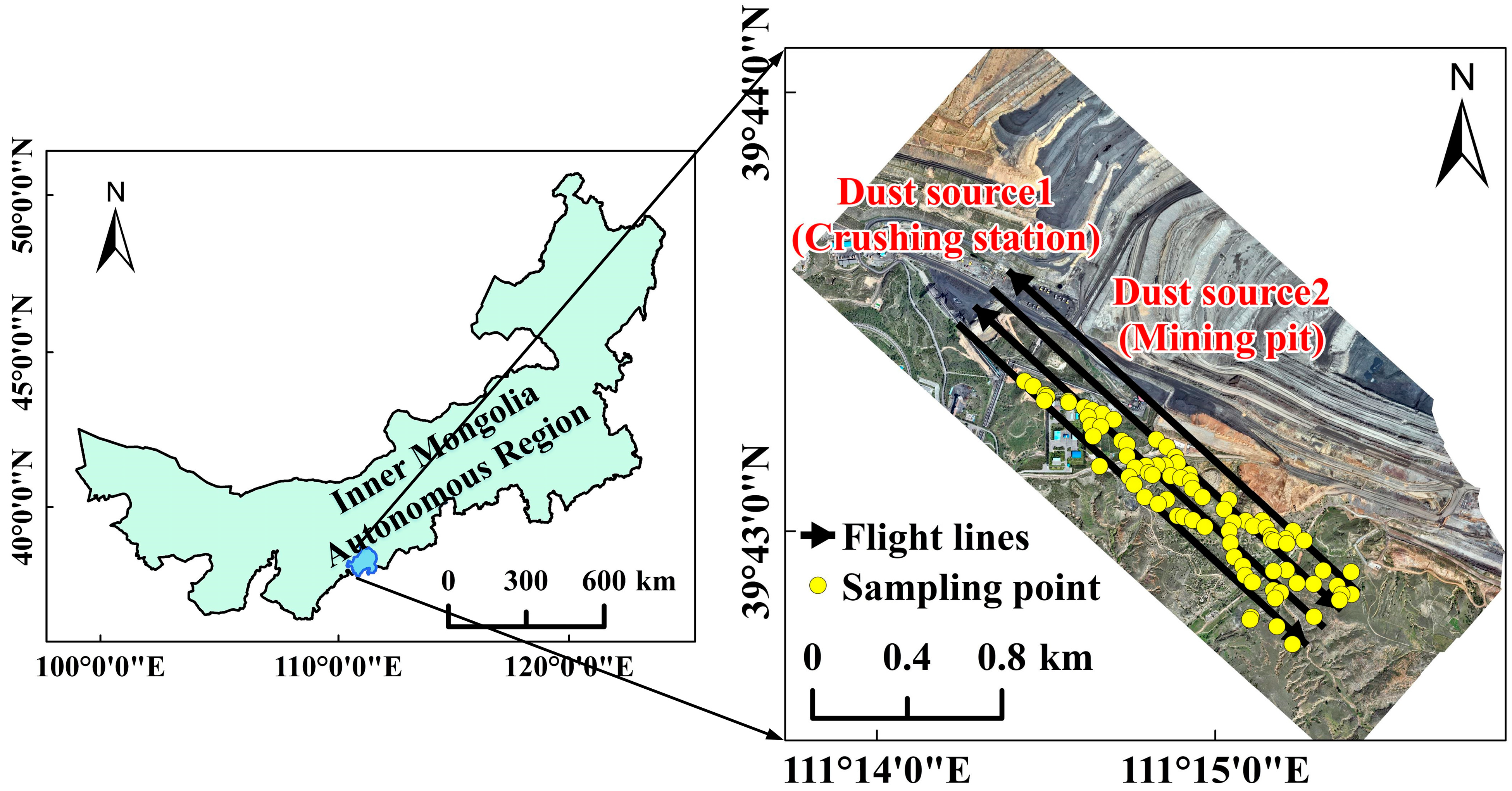
2.1. Study Area

The study site (111°14′50″ E, 39°43′13″ N) is situated in the southeastern part of Jungar Banner, Inner Mongolia, China (Figure 1). The central region has a higher elevation, while the northwest and southeast are relatively lower, with an altitude ranging from 1054 to 1192 m. It has a temperate continental monsoon climate, featuring abundant sunlight and clear seasonal variations. Winters are cold and prolonged, while summers are short and hot. Spring and autumn see considerable temperature changes, and the region receives limited precipitation, averaging 408 mm annually, compared to a much higher evapotranspiration rate of 2100 mm [29]. The primary soil types are yellow clay and sandy soil, both of which are poor in fertility, making the ecological environment quite fragile.

2.2. Canopy Dust Content Measurement

The experiment involved the simultaneous collection of 83 canopy dust samples during the acquisition of UAV-borne VNIR hyperspectral data. Five healthy leaves from the top of the plant were selected at each sampling point. After collection, the leaves were sealed in centrifuge tubes. Simultaneously, the samples’ coordinates were measured using a CHCNAV i70 GNSS receiver (CHCNAV, Shanghai, China), and relevant information, such as plant type and the surrounding environment, was recorded. After the samples were brought back to the laboratory, the initial weight of each sample point was measured using a balance with an accuracy of 1/10,000 g, denoted as $W_1$. Then, using a soft brush, the dust on the front surface of the leaves was carefully removed, and a second weighing was performed, recorded as $W_2$. Next, we used the leaf area meter (CID Bio-Science, New York, NY, USA) to measure the leaf area (cm²), denoted as S. The process of calculating the leaf dust content (LDC) was illustrated in Equation (1), and the mean value of dust content of all leaves within each sampling point was taken as the canopy dust content.

$$LDC\left(\mathrm{g}/{\mathrm{c}\mathrm{m}}^2\right)=\left(W_1-W_2\right)÷S\times 10000$$

(1)

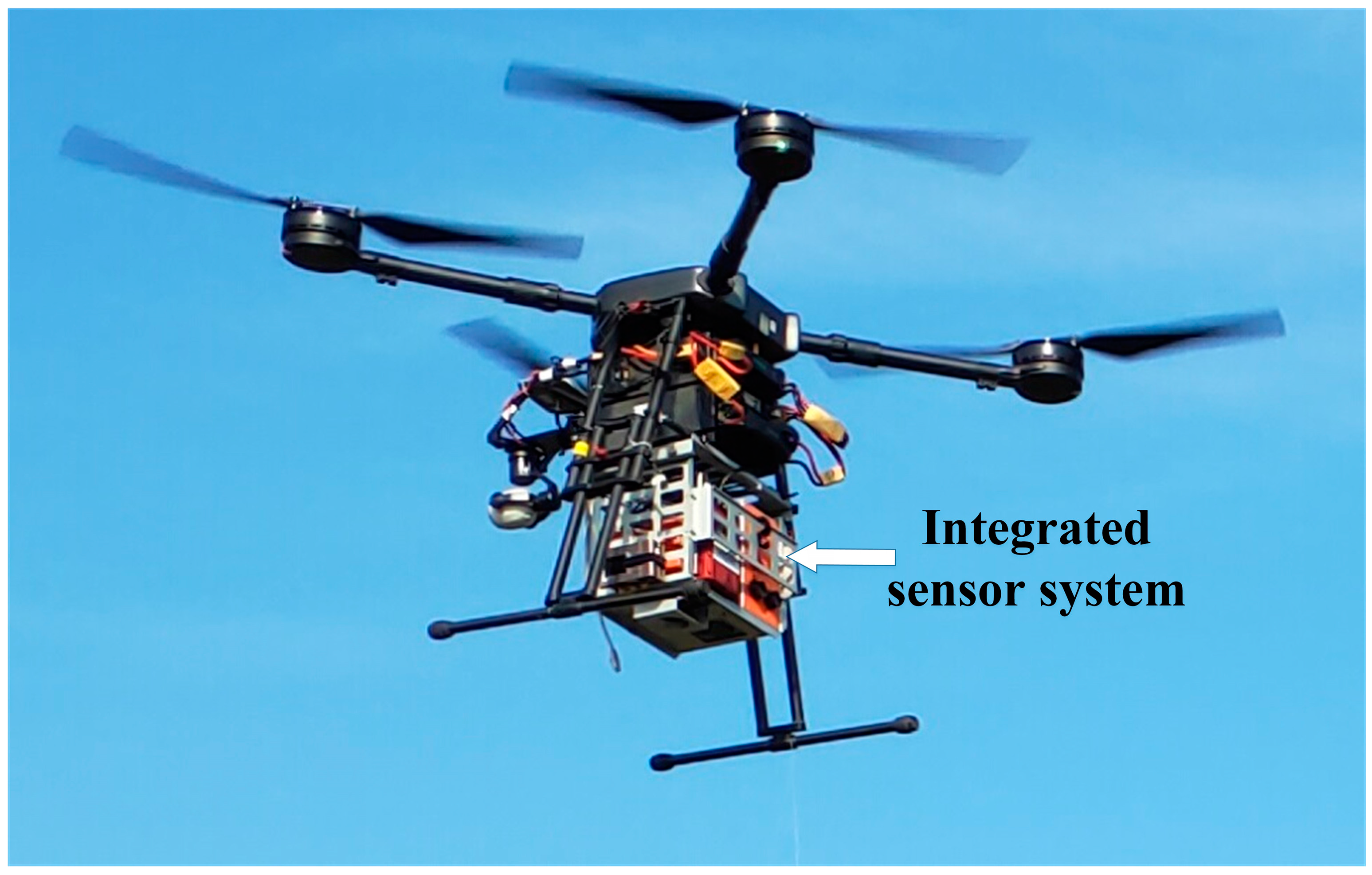
2.3. UAV-Borne VNIR Hyperspectral Image Collection and Processing

In this study, hyperspectral data were collected on 19 July 2024, between 11:00 AM and 12:00 AM using a Wind4 (DJI Technology, Shenzhen, China) equipped with an integrated sensor system. The Wind 4 is a quadrotor UAV with a total weight of 7.3 kg and a maximum take-off weight of 24.5 kg. A magnesium alloy bracket is installed beneath the UAV’s battery compartment to secure the integrated sensor system. The UAV and the integrated sensor system operate independently, with the UAV’s battery providing power to the integrated sensor system. The integrated sensor system consisted of an imaging spectrometer SPECIM FX10 (SPECIM, Oulu, Finland), a control system (DPU), as well as a global navigation satellite system (GNSS) and inertial measurement unit (IMU). Before the UAV takes off, the DPU is used to set parameters such as the flight lines, acquisition frequency, and exposure time. The GNSS and IMU can record the position and attitude of the imaging spectrometer. The SPECIM FX10 is a pushbroom imaging spectrometer capable of acquiring VNIR hyperspectral data with a high signal-to-noise ratio (SNR). It offers a spectral range of 400–1000 nm, a full-width half maximum (FWHM) of 5.5 nm, and a field of view (FOV) of 38°. The peak SNR can reach up to 600:1. The instrument weighs 1.4 kg and consumes less than 5 W of power. Since the GNSS and IMU can record the real-time position of the imaging spectrometer, the data collection task is automatically triggered when the UAV reaches the starting point of the flight lines. The collected hyperspectral data, along with the corresponding position and attitude data, are then saved to the hard disk mounted on the DPU. The installation of the UAV and the integrated sensor system is shown in Figure 2. The spectrometer’s binning mode was set to 4 × 2, and the flight altitude was set to 220 m above the ground; the parameters of the hyperspectral images are shown in

Table 1. Parameters of hyperspectral images.

Main Technical Details	Data
Spectral range (nm)	400–1000
Bands	112
Spectral sampling (nm)	3.4
Spatial sampling	512
Spatial resolution (m)	0.3
Size (GB)	14.2

. The flight area covers approximately 1.07 square kilometers and consists of 4 strips, with a 30% overlap between adjacent strips. Before utilizing UAV-borne VNIR hyperspectral data for canopy dust content inversion, data preprocessing is required. This process primarily consists of two steps, geometric correction and radiometric correction, with all operations carried out on a computer equipped with 64 GB of RAM and an Intel i9-13900K CPU.

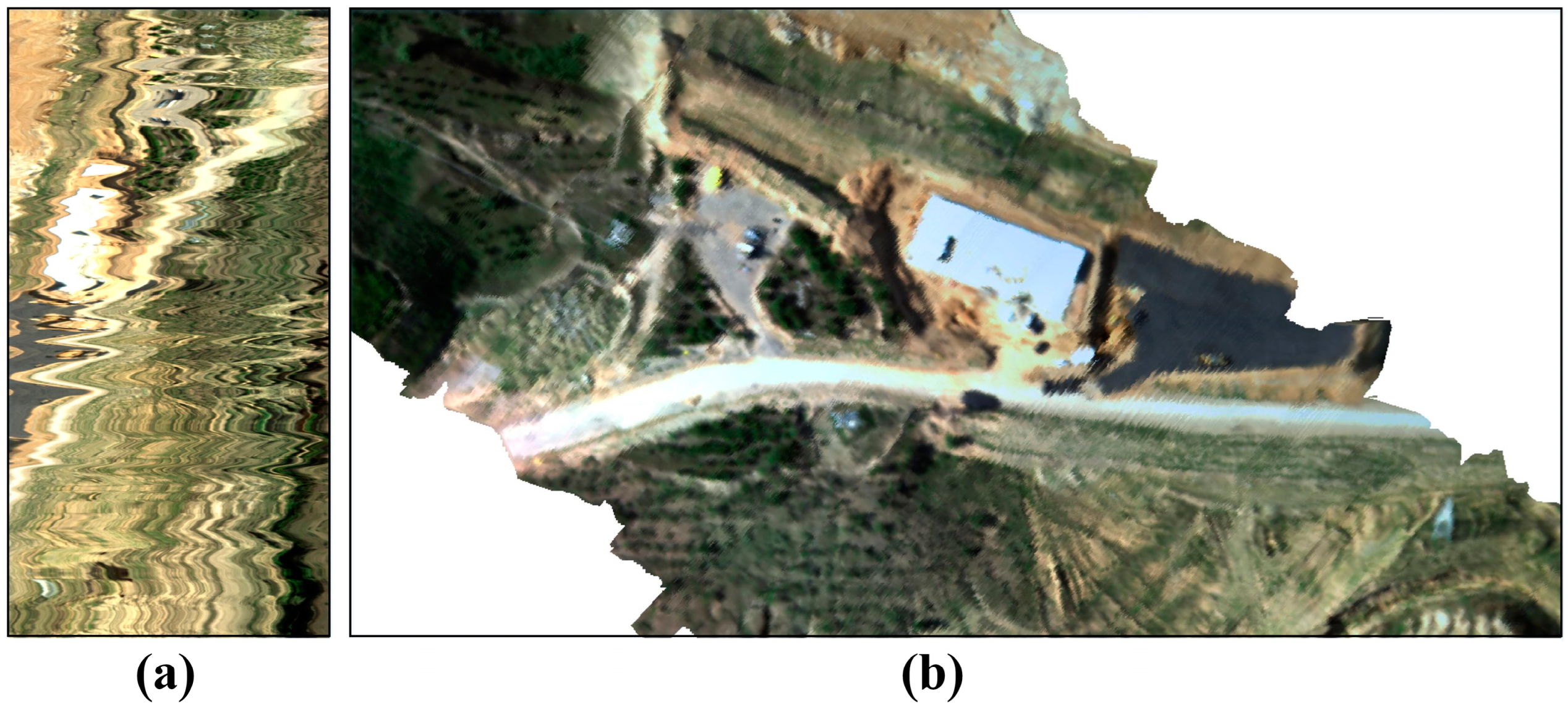
2.3.1. Geometric Correction

Factors such as UAV attitude changes and terrain variations often cause geometric distortions in hyperspectral data. The objective of geometric correction is to remove these distortions and restore the true spatial information. In this study, geometric correction is performed based on the collinearity equation, integrating position and attitude data from the inertial navigation system (INS) with the digital surface model (DSM). The DSM is generated using a Phantom 4 RTK (DJI Technology, Shenzhen, China) equipped with a high-resolution camera to capture overlapping images. These images are then processed with structure from motion (SFM) and multi-view stereo (MVS) techniques to reconstruct a 3D point cloud, which is subsequently interpolated to produce the final DSM. The detailed process is illustrated in Equation (2).

$$\left.\begin{array}{c}{X}_P=X_S+\left(Z_P-Z_S\right){\displaystyle \frac{a_{1}x+a_{2}y-a_{3}f}{c_{1}x+c_{2}y-c_{3}f}}\\ Y_P=Y_S+(Z_P-Z_S){\displaystyle \frac{b_{1}x+b_{2}y-b_{3}f}{c_{1}x+c_{2}y-c_{3}f}}\end{array}\right\}$$

(2)

where ($x$, $y$, $-f$) are the image space coordinates, ($X_P$, $Y_P$, $Z_P$) are the object space coordinates of the corresponding ground point, ($X_S$, $Y_S$, $Z_S$) are the object space coordinates of the sensor center, that is, the exterior orientation line elements, and $a_i$, $b_i$, $c_i$ (i = 1,2,3) are the rotation matrix elements, that is, the exterior orientation angle elements.

The geographic coordinates can be calculated once the exterior orientation elements are known. However, the position ($X_{IMU}$, $Y_{IMU}$, $Z_{IMU}$) obtained from the INS represents the location of the IMU center in the WGS84 coordinate system, while the attitude angles (${\theta }_r$, ${\theta }_p$, ${\theta }_h$) describe the attitude of the IMU coordinate system relative to the navigation system. To obtain the exterior orientation elements needed for geometric correction, a coordinate transformation is necessary. This transformation involves five coordinate systems: the geographic coordinate system (m), navigation coordinate system (g), IMU coordinate system (b), sensor coordinate system (c), and image space coordinate system (i).

The image space coordinate system takes the sensor’s perspective center as the origin, with the X-axis pointing in the UAV’s flight direction, the Y-axis pointing to the left side of the hyperspectral image, and the Z-axis pointing upwards along the sensor’s main optical axis. The Z-axis of the sensor coordinate system aligns with that of the image space coordinate system, but its Y-axis direction corresponds to the X-axis of the image space coordinate system, while the X-axis is opposite to the Y-axis direction of the image space coordinate system. The IMU coordinate system is a custom system with its origin defined according to the IMU manufacturer’s specifications. The X-axis points along the UAV’s flight direction, the Y-axis is perpendicular to the X-axis and points towards the UAV’s right wing, and the Z-axis, along with the X and Y axes, forms a right-handed coordinate system. The navigation coordinate system adopts the North-East-Down (NED) coordinate system, with the origin located at the phase center of the antenna. The X-axis points towards true north, the Y-axis points towards the Earth’s east, and the Z-axis points towards the Earth’s center along the ellipsoid’s normal vector. The geographic coordinate system adopts the WGS-84 coordinate system, with its origin at the Earth’s center of mass, including oceans and the atmosphere. The X-axis points to the intersection of the protocol meridian plane defined by BIH1984.0 and the CTP equator, the Z-axis points to the protocol Earth Pole (CTP) direction defined by the International Time Bureau BIH1984.0, and the Y-axis is determined according to the right-hand rule. The formula for calculating the exterior orientation angle elements is given in Equation (3), while the formula for the exterior orientation line elements is provided in Equation (4). The methods for calculating the variables in these equations can be found in references [30,31].

$$C_i^m\left(\phi ,\omega ,\kappa \right)=C_g^m{C}_b^g{C}_c^b{C}_i^c$$

(3)

$$\left[\begin{array}{c}\begin{array}{c}{X}_S\\ Y_S\end{array}\\ Z_S\end{array}\right]=C_g^m\left(\left[\begin{array}{c}\begin{array}{c}{X}_{IMU}\\ Y_{IMU}\end{array}\\ Z_{IMU}\end{array}\right]+C_b^g\left[\begin{array}{c}\begin{array}{c}{X}_l\\ Y_l\end{array}\\ Z_l\end{array}\right]\right)$$

(4)

where $C_i^m$ is the rotation matrix from the geographic coordinate system to the image space coordinate system, $C_g^m$ is the rotation matrix from the geographic coordinate system to the navigation coordinate system, $C_b^g$ is the rotation matrix from the navigation coordinate system to the IMU coordinate system, $C_c^b$ is the rotation matrix from the IMU coordinate system to the sensor coordinate system, and $C_i^c$ is the rotation matrix from the sensor coordinate system to the image space coordinate system. ($X_l$, $Y_l$, $Z_l$) is the eccentric vector of the sensor center in the IMU coordinate system, calculated by the GNSS and IMU.

To further improve the accuracy of the spatial coordinates in hyperspectral images, this study used a high-resolution orthophoto as the reference to register the hyperspectral images after geometric correction.

2.3.2. Radiometric Correction

The signal detected by UAV-borne VNIR hyperspectral sensors contains information from both the Earth’s surface and the atmosphere. Radiometric correction can remove the radiation distortions caused by the sensor, imaging environment, and atmosphere in hyperspectral images, thereby restoring the true radiative characteristics of ground objects. This process primarily involves three steps: radiometric calibration, atmospheric correction, and BRDF correction.

(1)

Radiometric calibration

Radiometric calibration converts the digital number (DN) recorded by the sensor into radiance, with the calculation process outlined in Equation (5) [32].

$$L={\displaystyle \frac{Gain\times [{DN}_o-Mean\left({DN}_d\right)-{DN}_s]}{Time}}$$

(5)

where $L$ is the radiance, measured in $\mathrm{m}\mathrm{W}{/(\mathrm{c}\mathrm{m}}^2·\mathrm{s}\mathrm{t}\mathrm{r}·\mathsf{\mu }\mathrm{m})$, Gain is the radiometric correction coefficient, ${DN}_o$ is the DN value of the original data, ${DN}_d$ is the DN value of the dark current, ${DN}_s$ is the DN value of the scattered light, and $Time$ is the integration time.

(2)

Atmospheric correction

Atmospheric correction can eliminate the effects of atmospheric absorption and scattering, converting radiance into reflectance [33,34]. According to the four-stream surface-atmosphere radiative transfer theory [35,36], reflectance for a Lambertian surface with homogeneous and flat land covers can be calculated using Equation (6). The parameters in the equation can be simulated using MODerate spectral resolution atmospheric TRANsmittance (MODTRAN) [37].

$$R={\displaystyle \frac{L-L_{path}}{G_t+G_b+S(L-L_{path})}}$$

(6)

where $R$ is the reflectance, $L$ is the radiance, $L_{path}$ is the path contribution, $G_t$ and $G_b$ are the gain factors for target and background, $S$ is the spherical albedo of the atmosphere.

(3)

BRDF correction

The reflectance of the Earth’s surface is influenced by sensor observation angle and solar illumination angle, with different angles potentially leading to varying reflectance values. BRDF correction can mitigate the radiometric differences caused by these angles, thus improving the radiometric consistency of hyperspectral images. In this study, the kernel-driven BRDF model is employed to describe the complex scattering mechanisms of the Earth’s surface, as shown in Equation (7) [38,39]. The BRDF parameters vary across different land cover types, necessitating their separate calculation for each type. To achieve this, this study utilizes atmospherically corrected hyperspectral data to classify the study area and generate a land cover map, which serves as the foundation for fitting BRDF parameters.

$$R\left({\theta }_o,{\theta }_s,{\phi }_o,{\phi }_s,c,\lambda \right)=f_{iso}\left(c,\lambda \right)+f_{vol}\left(c,\lambda \right)k_{vol}\left({\theta }_o,{\theta }_s,{\phi }_o,{\phi }_s\right)+f_{geo}\left(c,\lambda \right)k_{geo}\left({\theta }_o,{\theta }_s,{\phi }_o,{\phi }_s\right)$$

(7)

where $R\left({\theta }_o,{\theta }_s,{\phi }_o,{\phi }_s,c,\lambda \right)$ is the simulated reflectance at the observed geometry, $f_{iso}$ is the isotropic scattering coefficient, $k_{vol}$ and $f_{vol}$ are the volumetric scattering kernel and coefficient, $k_{geo}$ and $f_{geo}$ are the geometric-optical kernel and coefficient, ${\theta }_o$ is the observe zenith angle, ${\theta }_s$ is the solar zenith angle, ${\phi }_o$ is the observe azimuth angle, ${\phi }_s$ is the solar azimuth angle, $c$ is the land-cover type, and $\lambda$ is the wavelength.

Using the Li–Transit–Reciprocal (LTR) kernel [40,41] as the geometric-optical kernel and the hotspot-revised Ross–Thick–Maignan (RTM) kernel [38,42] as the volumetric scattering kernel, the reflectance ratio between the observation direction and reference direction, i.e., the anisotropy factor (ANIF), is calculated using Equation (8). The BRDF-corrected reflectance is then obtained through Equation (9).

$$ANIF={\displaystyle \frac{R\left({\theta }_o,{\theta }_s,{\phi }_o,{\phi }_s,c,\lambda \right)}{R\left({\theta }_o=0°,{\theta }_s={\theta }_{s\_mean},{\phi }_o=0°,{\phi }_s={\phi }_{s\_mean},c,\lambda \right)}}$$

(8)

$$R_c={\displaystyle \frac{R}{ANIF}}$$

(9)

where $R\left({\theta }_o,{\theta }_s,{\phi }_o,{\phi }_s,c,\lambda \right)$ is the simulated reflectance at the observed geometry, $R\left({\theta }_o=0°,{\theta }_s={\theta }_{s\_mean},{\phi }_o=0°,{\phi }_s={\phi }_{s\_mean},c,\lambda \right)$ is the simulated reflectance at the reference geometry, ${\theta }_{s\_mean}$ is the mean solar zenith angle for all strips, and ${\phi }_{s\_mean}$ is the mean solar azimuth angle for all strips; $R$ is the image’s original reflectance, and $R_c$ is the BRDF-corrected reflectance.

Finally, using a georeferenced mosaicking method, all the flight strips were mosaicked together to create an orthophoto covering the entire study area. Extract the spectral curves of the pixels corresponding to the sampling points from the hyperspectral data using the field-measured coordinates.

2.4. Spectral Transformation and Characteristic Bands Selection

To reduce noise interference and effectively highlight spectral features, the raw hyperspectral data underwent five transformations: FD, SD, LT, RT, and SR. The CARS method was used to extract characteristic bands for canopy dust content from both the original spectra and those after five transformations. CARS is a band selection algorithm that iteratively adjusts weights through competitive and adaptive sampling. In each iteration, it retains the points with larger absolute regression coefficient weights in the PLSR model as the new feature subset, while discarding poorly performing subsets [43,44]. Although CARS requires extensive resampling and multiple iterations, leading to high computational costs and sensitivity to parameter selection, and does not consider the correlation between bands, it efficiently selects key features by removing redundant and irrelevant variables, while dynamically adjusting feature band weights. This enhances the stability and reliability of the selection process, making CARS a widely adopted method in feature selection [45,46]. Canopy dust content was considered the dependent variable in this research, while characteristic bands from various transformations were used as independent variables to develop the hyperspectral inversion models.

2.5. Model Construction and Evaluation

The canopy dust content inversion models were constructed using four methods: PLSR, ELM, SVM, and RF.

PLSR maximizes the covariance between the independent variables and the dependent variable by projecting the independent variables onto a set of new latent variables. Unlike conventional regression methods, PLSR can handle highly correlated independent variables and multicollinearity issues [47,48]. Although PLSR is hindered by poor interpretability, high computational costs, and the need for expert knowledge in parameter selection, it excels in efficiently modeling with a limited number of samples. It effectively addresses multicollinearity, reduces the dimensionality of the feature space, and enhances model stability. Additionally, PLSR’s ability to handle multiple response variables simultaneously has contributed to its widespread use in surface parameter estimation [49,50].

The ELM is an improved algorithm based on the theory of single-layer feedforward neural networks [51,52]. Although the ELM faces challenges such as limited interpretability of its model structure, sensitivity to noise, and a lack of a clear parameter optimization mechanism, it offers notable advantages for handling large-scale data. The ELM can be trained quickly, with relatively low requirements for sample size and feature count, enabling good predictive performance even with limited samples. Additionally, the ELM is computationally efficient and less prone to overfitting, making it especially suitable for big data and real-time prediction tasks. Its efficient training process and strong generalization capability have led to its widespread application in classification [53], regression [54], and pattern recognition [55] tasks.

The SVM maps the vectors to a high-dimensional feature space through nonlinear transformation and uses cross-validation and grid search methods to optimize parameters. It seeks the optimal hyperplane in the feature space to achieve regression prediction for the dependent variable [56,57]. Although the SVM has some limitations, such as relatively high computational costs, sensitivity to the choice of kernel, and challenges in handling large datasets with many features, it is particularly effective in high-dimensional spaces and well suited for cases where the number of features exceeds the number of samples. Its ability to find the optimal hyperplane that maximizes the margin between classes makes it highly accurate and robust against overfitting, especially with proper regularization. As a result, the SVM offers significant advantages in both classification [58,59] and regression [60,61] tasks.

RF is a regression method based on the ensemble learning principle. Its core idea is to build multiple decision trees and combine their prediction results to improve the model’s accuracy and stability. The training data for each tree are randomly sampled from the original dataset using the bootstrap method. The final prediction value is obtained by averaging the predictions or taking the mode of the multiple decision trees’ results [62,63]. Despite its limitations, such as high computational cost and challenges in model interpretability, RF excels at handling high-dimensional data and capturing complex relationships between features without the need for extensive data preprocessing. By integrating multiple decision trees, RF improves model accuracy and robustness while minimizing the risk of overfitting. Its outstanding performance in classification and regression tasks has led to its widespread adoption in areas such as peatland ecosystem mapping [64] and quantitative inversion [65,66], making it the preferred method in many application scenarios.

This study used the coefficient of determination ($R^2$), root mean square error (RMSE), and relative prediction deviation (RPD) to evaluate the model’s prediction results [67].

3. Results

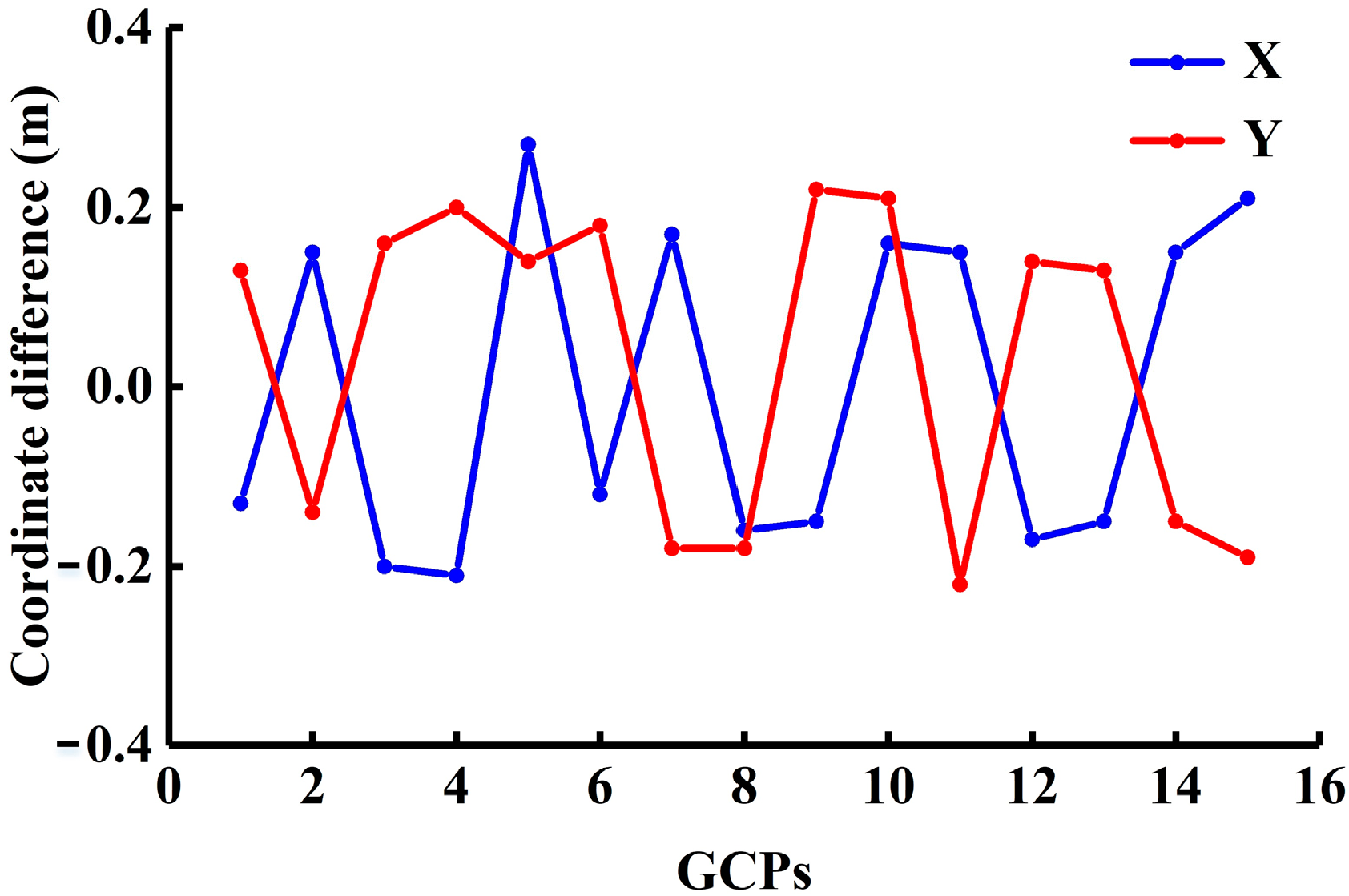
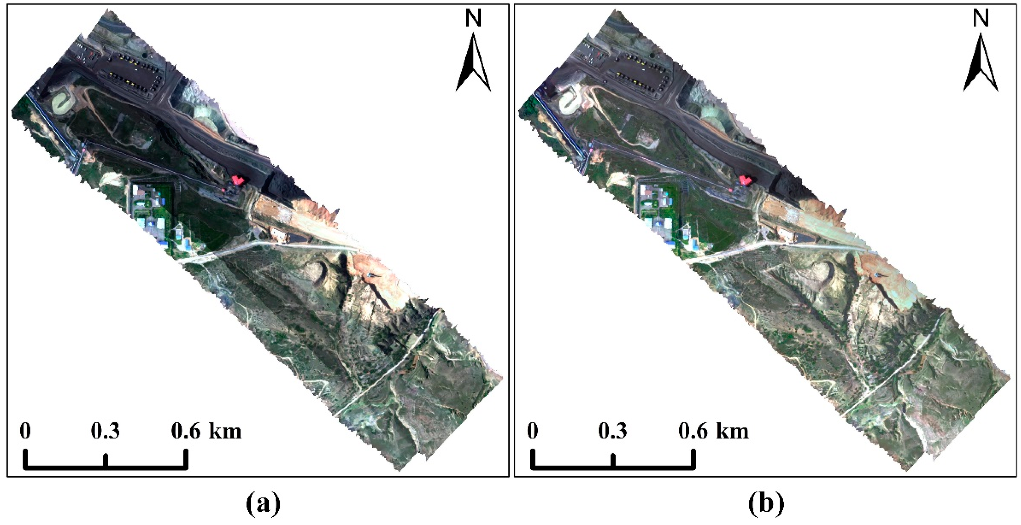
3.1. Evaluation of Geometric Correction for UAV-Borne VNIR Hyperspectral Data

Figure 3 shows a comparison of partial hyperspectral data before and after geometric correction. Due to frequent changes in sensor attitude caused by UAV vibrations and airflow, the pre-corrected images exhibit severe distortion and stretching, leading to confusion in the relative positions of ground objects. Furthermore, the pre-corrected image lacks spatial coordinate information, making it difficult to accurately extract relevant features based on geographic coordinates. After geometric correction, the image restores the correct relative position relationships and incorporates geographic coordinate information, making texture features more prominent and significantly enhancing the image’s usability and analytical accuracy. Figure 4 illustrates the differences between the image coordinates and the measured coordinates for 15 Ground Control Points (GCPs). The absolute coordinate differences in both the X and Y directions are less than 0.27 m, and the RMSE for all GCPs is 0.25 m, which is smaller than the width of a pixel. This indicates that the geometric correction is highly accurate, ensuring the precise extraction of feature information.

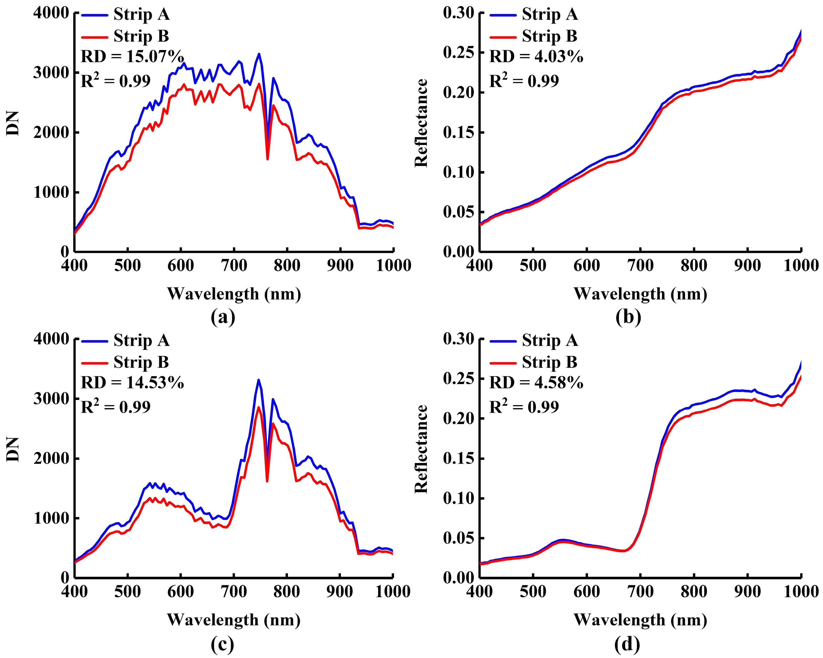
3.2. Evaluation of Radiometric Correction for UAV-Borne VNIR Hyperspectral Data

Figure 5 presents the UAV-borne VNIR hyperspectral images before and after radiometric correction. Due to differences in illumination–observation geometry, atmospheric conditions, and other factors, there are significant radiometric discrepancies between adjacent strips in the uncorrected data. Moreover, the overall brightness of the uncorrected images is lower due to the influence of shadow occlusion, which partially obscures the true reflective characteristics of ground objects and complicates subsequent data interpretation. After radiometric correction, not only are the radiometric differences between adjacent strips eliminated, but the overall brightness of the image is also significantly enhanced, allowing for the clear restoration of surface object reflectance characteristics and improving the image’s usability and accuracy.

Figure 6 shows an example of the reflectance curves for co-located points in adjacent strips. Before radiometric correction, the spectral values of strip A were consistently higher than those of strip B. Although the reflectance curves for co-located points were similar and the R² value exceeded 0.99, significant discrepancies in absolute values were observed. Specifically, the relative deviation (RD) for bare soil reached 15.07%, while for plant it was 14.53%. After radiometric correction, the reflectance differences between co-located points were significantly reduced. These results indicate that radiometric correction not only eliminates the effects of atmospheric absorption and scattering but also effectively mitigates reflectance heterogeneity caused by differences in illumination and observation angles.

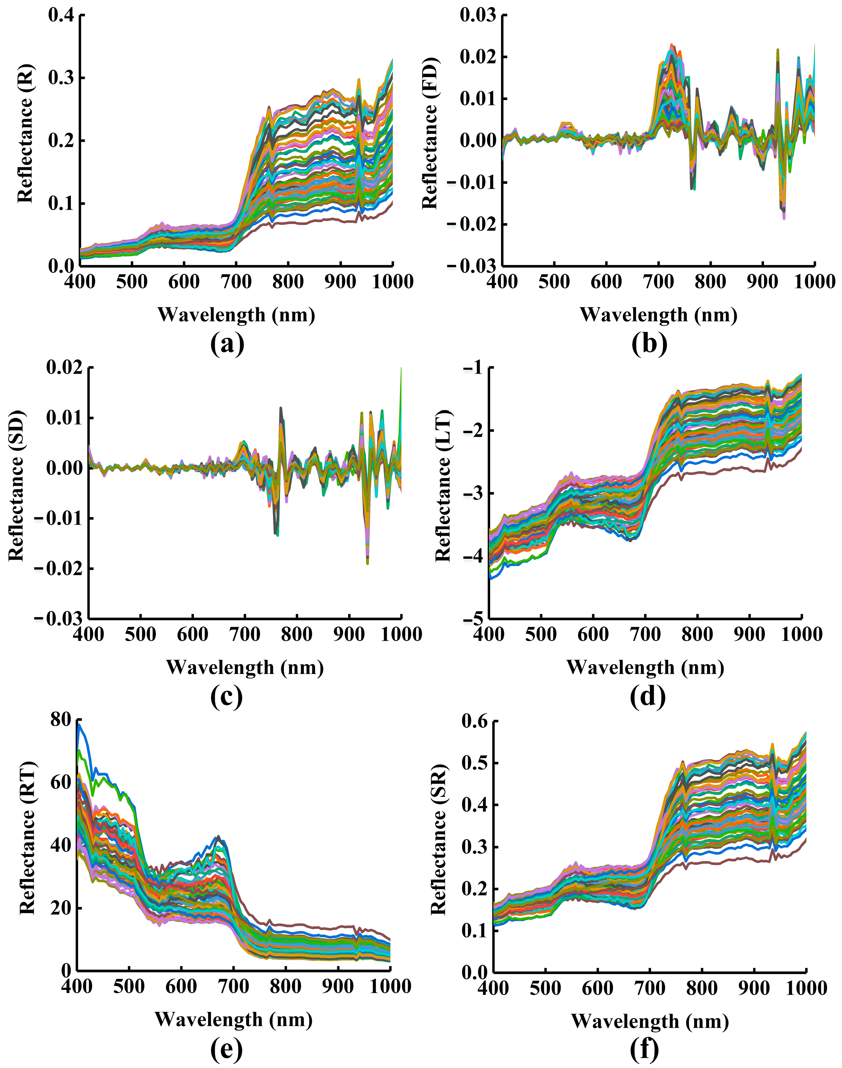
3.3. Feature Analysis Before and After Spectral Transformation

Figure 7 shows the original spectrum and its transformed versions. The original spectral curve is smooth, with chlorophyll strongly absorbing blue and red light, while reflecting green light more significantly. This results in a small reflection peak around 550 nm and absorption peaks at 450 and 680 nm. Near-infrared light is scattered multiple times within the leaf’s internal cellular structure, leading to increased reflectance in the near-infrared wavelength. However, around 970 nm, water absorption causes a slight decrease in reflectance. The band between red light and near-infrared wavelength (680–750 nm) shows a steep rise, known as the “red-edge”. The spectra after logarithm and square root transformations resemble the original spectra in shape. These two transformations highlight the mixed spectral features by compressing high reflectance values or balancing the reflectance distribution. However, after these transformations, the differences in the visible range increase, while those in the near-infrared range decrease. The spectrum after reciprocal transformation reveals significantly higher values in the visible range compared to the near-infrared range. The first derivative calculates the rate of change between adjacent bands, and the second derivative calculates the rate of change in the curvature of the spectral curve. Therefore, the curve exhibits more pronounced fluctuations, with a noticeable increase in peaks and valleys [68].

The average absolute values of the correlation coefficients between the original spectra and those after FD, SD, LT, RT, and SR transformations, and canopy dust content, are 0.09, 0.12, 0.13, 0.13, 0.19, and 0.11, respectively. This indicates that spectral transformations significantly enhance the correlation between the spectrum and canopy dust content, thereby improving the accuracy of dust monitoring.

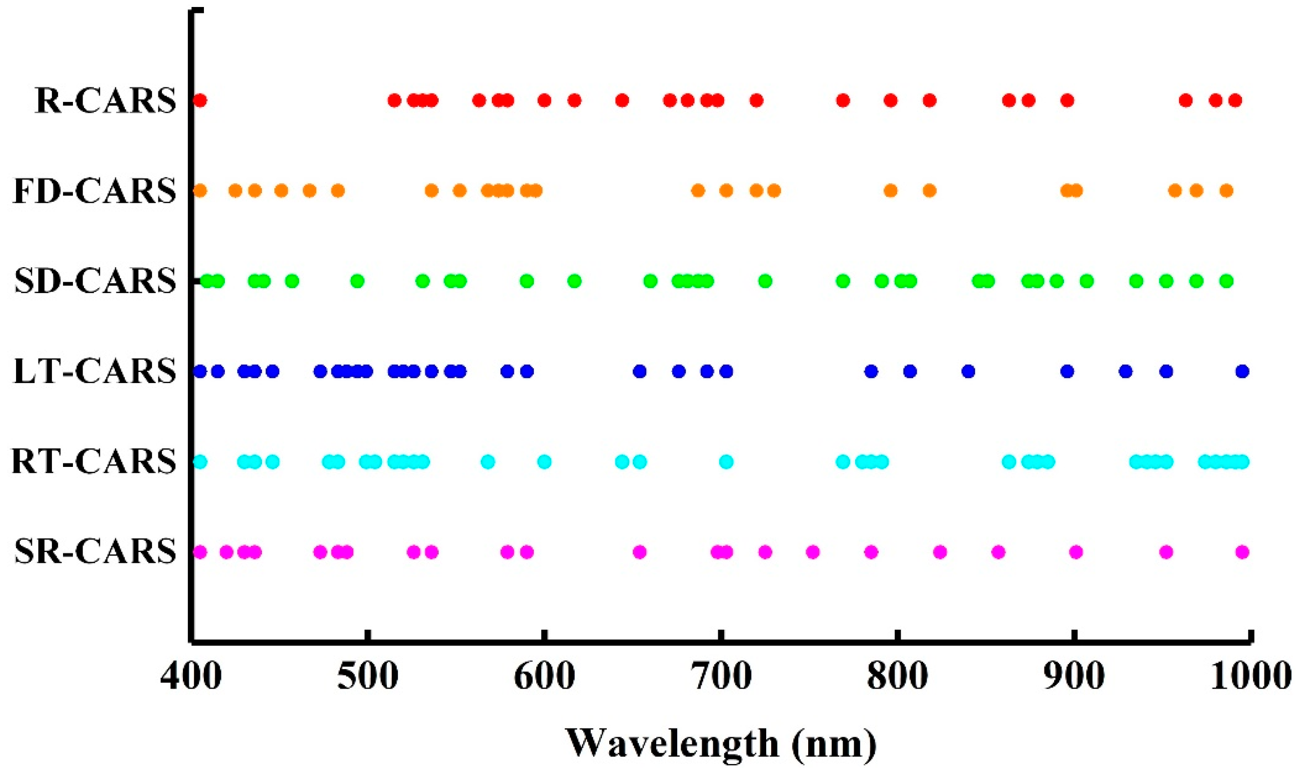
3.4. Characteristic Band Selection

CARS follows the “survival of the fittest” principle, selecting the most representative feature variables [69]. In this study, the number of Monte Carlo sampling iterations was set to 50, with 10-fold cross-validation and 1000 iterations. The number of characteristic bands chosen from both the original and transformed spectra ranged from 22 to 34, with the specific distribution shown in Figure 8. The results show that the characteristic bands selected by the CARS algorithm account for 20 to 30% of the total 112 bands and are evenly spread across the entire spectral range, effectively reducing the computational complexity of the inversion model.

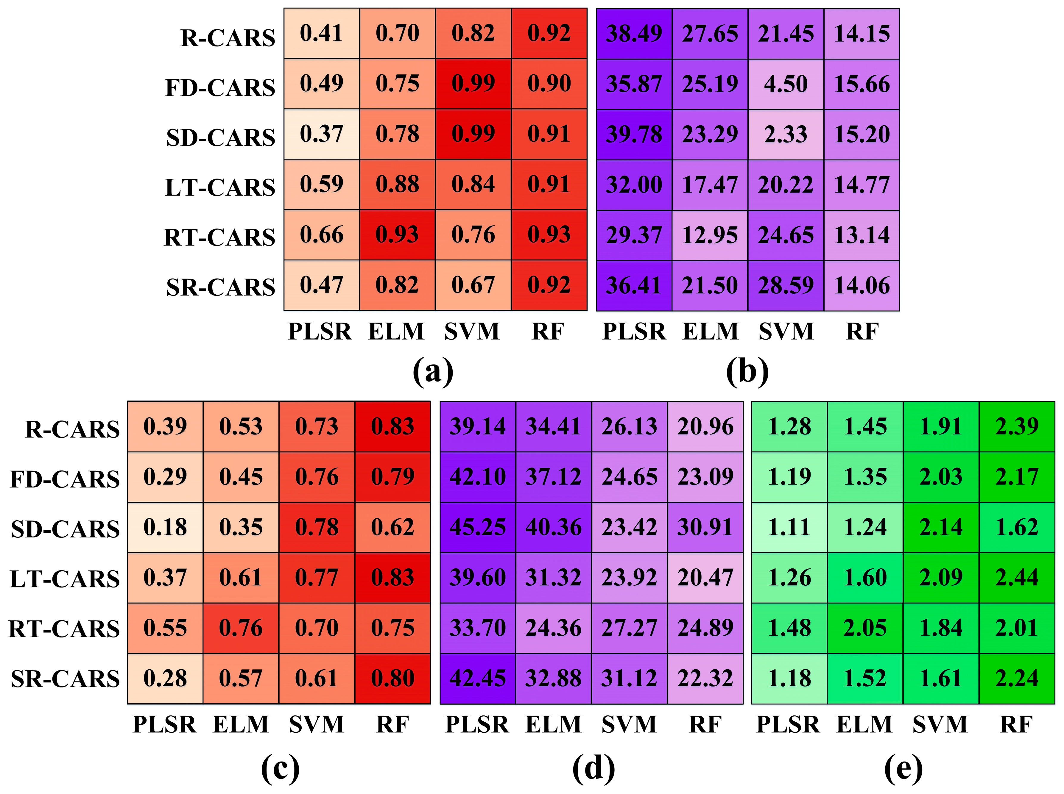
3.5. Construction of the Canopy Dust Content Inversion Model

The accuracy of the canopy dust content inversion models constructed using the characteristic bands combined with PLSR, ELM, SVM, and RF methods, is shown in Figure 9. Both feature extraction and modeling methods influence the inversion accuracy. For the calibration set, the model built using the reciprocal-transformed spectra exhibited the highest inversion accuracy, while the model built using the original spectra performed the worst. This indicates that the transformed spectra effectively enhanced the canopy dust feature, improving inversion accuracy. The model built using logarithm-transformed spectra best-predicted canopy dust content for the validation set, while the second derivative spectra performed the worst. Among the four modeling methods, the overall inversion performance, from best to worst, is RF, SVM, ELM, and PLSR. The optimal inversion results were achieved using the LT-CARS and RF combination, with R² and RMSE values of 0.91 and 14.77 for the calibration set, respectively. For the validation set, the R² and RMSE were 0.83 and 20.47, with an RPD of 2.44. These results indicate that the model possesses robust predictive power and can effectively estimate canopy dust content.

4. Discussion

4.1. Experimental Accuracy Analysis

Hyperspectral data offer rich spectral information but are often characterized by a large number of bands and high dimensionality. This study applies the CARS method to select characteristic bands from hyperspectral data and constructs a canopy dust content inversion model. Compared to using all available bands, the feature band selection approach effectively reduces redundancy and noise, lowers data dimensionality, and mitigates the computational burden and information redundancy associated with high-dimensional data. However, the feature selection process may lead to the loss of some bands, which could cause the model to perform suboptimally in certain specific scenarios. Therefore, future research should carefully balance the trade-off between hyperspectral data dimensionality, computational efficiency, and accuracy in order to develop more effective canopy dust content inversion models.

In the study of hyperspectral remote sensing inversion of plant canopy dust content, the ranking of spectral transformation and modeling methods is influenced by factors such as data characteristics, SNR, background interference, model adaptability, and overfitting risk. In the calibration set, RT outperforms SD, FD, LT, SR, and the original spectral, as it enhances information in low-reflectance regions and improves the model’s generalization ability [70,71]. In contrast, the original spectrum is most susceptible to noise. In the validation set, both the RT and LT perform best, while SD ranks last due to overfitting [72,73]. Regarding modeling methods, the rankings of RF, SVM, ELM, and PLSR. RF performs the best due to its strong feature selection capability and robustness to high-dimensional data [62,63], while SVMs, although effective for nonlinear fitting, have higher computational complexity [74]. ELMs are less stable, and PLSR, as a linear model [75,76], struggles with nonlinear hyperspectral data. The differences in spectral transformation rankings between the calibration and validation sets are mainly due to overfitting and model adaptability. The RT proves to be the best method in both sets. Overall, spectral transformation impacts the model’s learning and generalization ability, while the modeling method determines the fitting accuracy. Together, these factors influence the overall performance of the model.

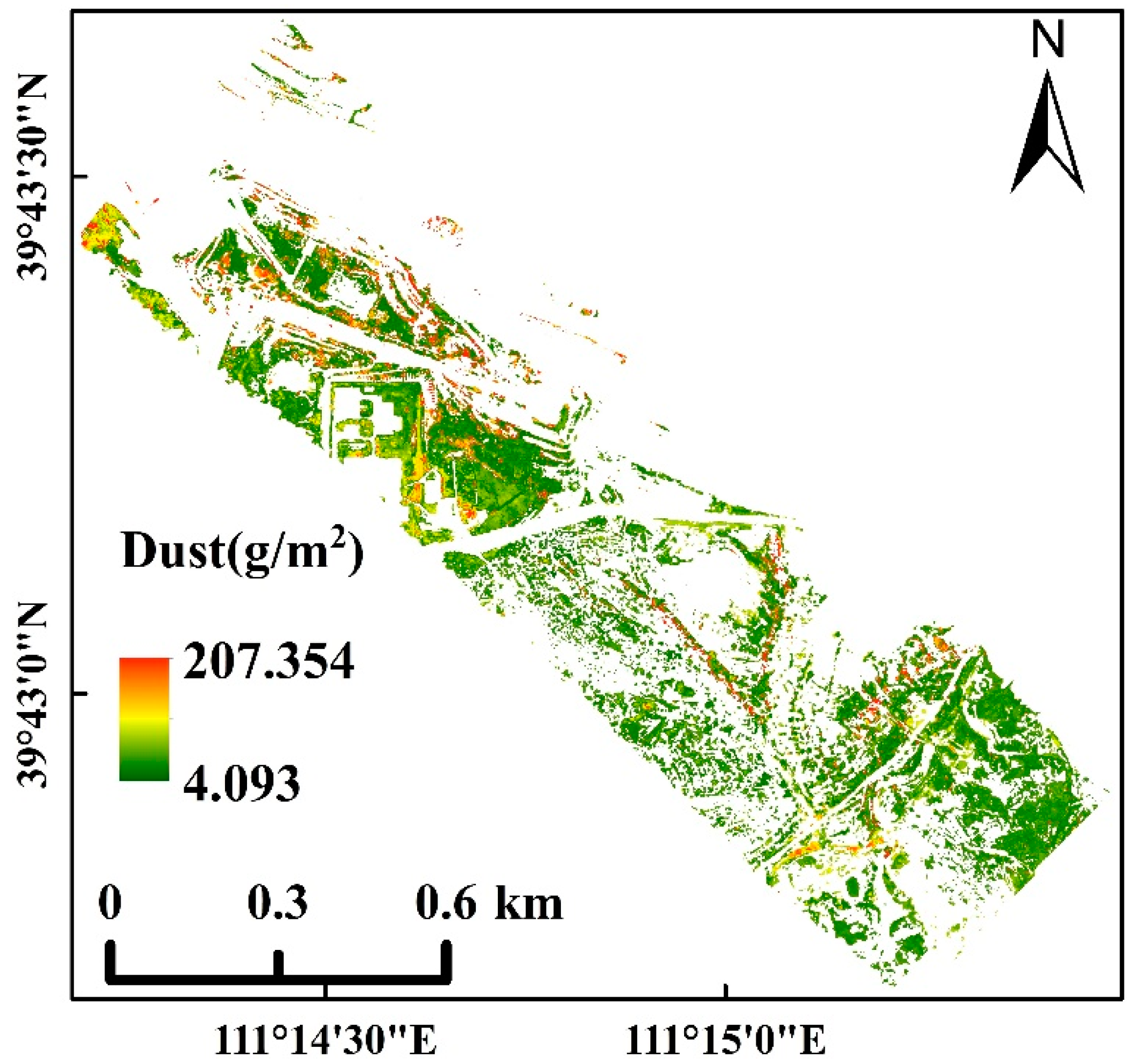
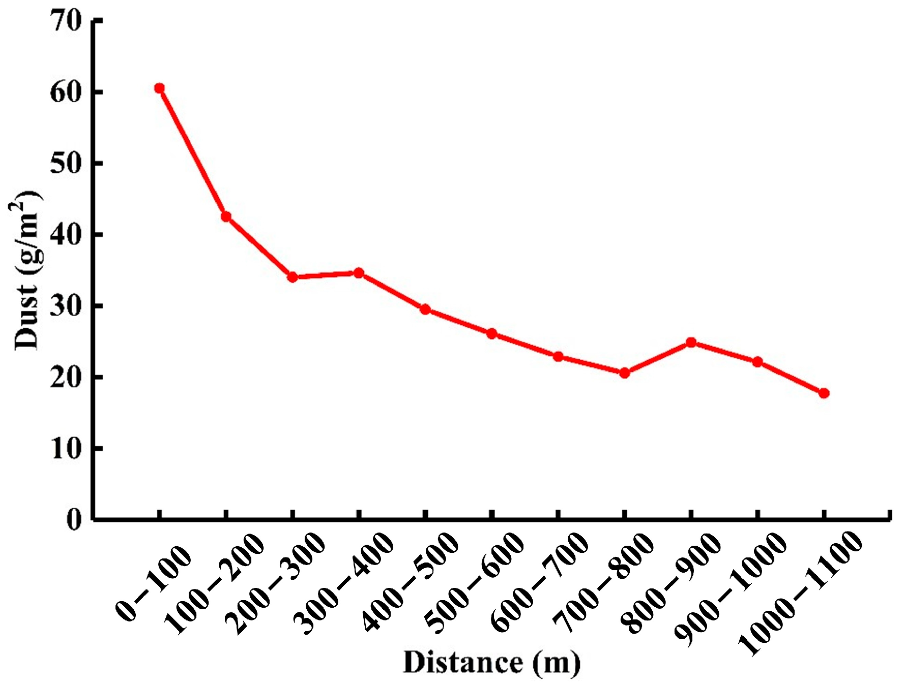
4.2. Spatial Distribution Characteristics of Canopy Dust Content

In this study, a supervised classification approach was employed to categorize the hyperspectral image into 15 classes, and the classification accuracy is shown in

Table 2. Classification accuracy of the UAV-borne VNIR hyperspectral image.

Class Names	Value	Class Names	Value	Class Names	Value
Building	99.28	Gravel	78.13	Elm	91.67
Pavement	83.72	Apple tree	75.00	Feather grass	100.00
Artemisia	80.72	Apricot tree	86.67	False indigo	83.33
Elymus grass	93.94	Bare soil	97.44	AA	87.71
Willow	75.00	Peach tree	80.00	OA	91.26
Mine	90.70	Poplar	100.00	Kappa	0.90

. The average accuracy, overall accuracy, and kappa coefficient were 87.71%, 91.26%, and 0.90, respectively, indicating that the different land cover types in the image were accurately distinguished. This provides an effective foundation for subsequent canopy dust content inversion and spatial distribution analysis. The optimal canopy dust content inversion model was applied to the plant area, deriving the corresponding spatial distribution map of canopy dust content, as shown in Figure 10. The canopy dust content range obtained by hyperspectral image inversion is 4.09–207.35 g/m², with the windward slope exhibiting significantly higher dust content than the leeward slope. This result suggests that under the influence of wind, more dust accumulates on the windward slope, while the leeward slope experiences less dust content due to weakened wind.

To further investigate the connection between canopy dust content and distance from dust sources, this study used the mining pit and crushing station as the centers of buffer zones. A 100 m interval was used to determine the mean value of dust content in each buffer zone (Figure 11), with values ranging from 17.75 to 60.50 g/m². Canopy dust content typically decreased as the distance from the dust source increased. This trend aligns with the dust dispersion process: under wind influence, dust spreads, with larger particles settling first due to gravity, while smaller particles continue to disperse and gradually settle. Therefore, dust content diminishes with distance from the source. In summary, the dust content’s distribution is influenced by various factors, such as terrain, wind direction, dust source location, and particle size. By integrating hyperspectral imaging with dust content inversion models, the spatial distribution of dust content can be effectively mapped, offering valuable insights for environmental monitoring and pollution control.

4.3. Limitation and Future Work

The CARS algorithm is effective for feature band selection but may not fully consider the correlation between bands, as it evaluates them individually based on their importance, typically measured by regression coefficients. This can lead to suboptimal feature selection, particularly when multiple correlated bands offer complementary information. To address this limitation, we plan to integrate CARS with decorrelation algorithms in the future to account for band correlations, reduce redundancy, and enhance feature selection.

We have only used VNIR hyperspectral data to invert plant canopy dust content. In the future, we plan to incorporate SWIR hyperspectral data. The SWIR bands can significantly enhance spectral feature extraction, particularly in distinguishing the reflectance characteristics between plant leaves and dust, thus reducing background interference. Furthermore, SWIR bands’ light strongly reflects dust and other non-biological substances, which can improve the model’s robustness and enhance its ability to generalize in complex environments.

In this study, the relationship between canopy dust content and the distance from the dust source was analyzed without taking into account meteorological data and other influencing factors. In the future, we plan to collect hyperspectral images over multiple periods and from larger areas, and perform an in-depth analysis of how the canopy dust content correlates with the distance from the dust source under varying meteorological conditions.

5. Conclusions

This research presents an approach for inverting canopy dust content in mining areas using UAV-borne VNIR hyperspectral images. The study involves performing precise geometric and radiometric corrections on the hyperspectral data to ensure accuracy. Characteristic bands are extracted through spectral transformations and the CARS method, followed by the construction of inversion models using regression techniques. The spatial distribution of canopy dust content is then analyzed. This approach provides valuable insights into dust management in mining regions and highlights the potential of hyperspectral imagery in environmental monitoring and land reclamation efforts. The main conclusions are as follows:

(1)

The geometric correction of the UAV-borne VNIR hyperspectral images accurately restored the true spatial information, revealing more distinct texture features. The absolute differences between the image coordinates of the GCPs and their measured coordinates are less than 0.270 m, with an RMSE of 0.246 m for all GCPs, demonstrating high positional accuracy.

(2)

Following radiometric correction, the UAV-borne VNIR hyperspectral image effectively mitigates the effects of sensor, atmospheric, and illumination–observation angle distortions. This correction restores the true reflectance information, enhances the overall brightness of the image, and improves consistency between adjacent strips.

(3)

Spectral transformation effectively enhances canopy dust feature information. The characteristic bands extracts by the CARS algorithm account for 20 to 30% of the total bands and are evenly distributed across the full spectral range, significantly reducing the computational complexity of the inversion model.

(4)

The accuracy of canopy dust content inversion is influenced by both feature extraction methods and modeling approaches. The optimal inversion model is obtained by combining LT-CARS and RF. This model exhibits strong predictive capability and can accurately invert canopy dust content. Canopy dust content decreases as the distance from the dust source increases.

As a suggestion, the mining area should prioritize controlling dust emissions at the source and minimizing dust discharge. Spray dust suppression should be implemented in key areas, while greening and covering measures can effectively mitigate dust release. Regular removal of accumulated dust can be achieved through mechanical sweeping equipment. Additionally, a real-time monitoring system should be established to dynamically adjust dust control measures based on data feedback. Efforts should also be made to strengthen public environmental awareness and enhance employee training on environmental practices.

References

1. Edenhofer, O. King Coal and the queen of subsidies. Science 2015, 349, 1286–1287. [Google Scholar]
2. Li, Q. Progress of ecological restoration and comprehensive remediation technology in large-scale coal-fired power base in the eastern grassland area of China. J. China Coal Soc. 2019, 44, 3625–3635. [Google Scholar]
3. Zhu, J.; Liang, C.; Zhu, G.; Wang, C.; Xu, H.; Wang, L. Preparation and long-term filtration performance of PLA-based nanofibrous membrane filters for ultra low-resistance respir-atory protection. J. China Coal Soc. 2024, 49, 1952–1963. [Google Scholar]
4. Lu, J.; Lei, S. Research Overview of Effect of Dust on Environment and Its Diffusion Laws in Open-Pit Coal Mine. Saf. Coal Mines 2017, 48, 231–234. [Google Scholar]
5. Ahrens, M.J.; Morrisey, D.J. Biological effects of unburnt coal in the marine environment. In Oceanography and Marine Biology; CRC Press: Boca Raton, FL, USA, 2005; pp. 79–132. [Google Scholar]
6. Fan, Q.; Li, S.; Guan, T.; Wu, X.; Wang, R.; Ren, L. The ecological effect on plant and soil around opencast coal mine from the mineral dust. Environ. Dev. 2013, 25, 104–108. [Google Scholar]
7. Li, Y.; Zhao, N.; Cao, Y.; Yang, J. Effects of coal dust deposition on the physiological properties of plants in an open-pit coal mine. Acta Ecol. Sin. 2018, 38, 8129–8138. [Google Scholar]
8. Tezara, W.; Habash, D.; Paul, M.J.; Lawlor, D.W. Effects of water stress on the biochemistry and physiology of photosynthesis in sunflower. Photosynth. Res. 1995, 205, 625–628. [Google Scholar]
9. Yang, H.; Wei, L.; Ye, X.; Liu, G.; Yang, X.; Huang, Z. Effects of coal dust deposition on seedling growth of Hedysarum laeve Maxim., a dominant plant species on Ordos Plateau. Acta Ecol. Sin. 2016, 36, 2858–2865. [Google Scholar]
10. Li, D.; Zhao, Z.; Guo, S.; Zheng, L.; Zhang, X.; Sui, J. “13th Five-Year Plan” coal mine dust occupational hazard prevention and control technology and development direction. Min. Saf. Environ. Prot. 2022, 49, 51–58. [Google Scholar]
11. Guo, H.; Cheng, Y.; Ren, T.; Wang, L.; Yuan, L.; Jiang, H.; Liu, H. Pulverization characteristics of coal from a strong outburst-prone coal seam and their impact on gas desorption and diffusion properties. J. Nat. Gas Sci. Eng. 2016, 33, 867–878. [Google Scholar]
12. Yun, A.; Jinqing, Z.; Haijuan, Z.; Ruizhen, D. Research progress on the influencing factors and response mechanisms of plant adsorption of atmospheric particulate matter. Yingyong Shengtai Xuebao 2024, 35, 2013. [Google Scholar]
13. Xiao, H.; Chen, X.; Ling, Q.; Zhou, Z. Analysis of dust detention capability of landscape plants and the hyperspectral remote sensing quantitative models construction of foliagedust detention. Resour. Environ. Yangtze Basin 2015, 24, 229–236. [Google Scholar]
14. Brackx, M.; Van Wittenberghe, S.; Verhelst, J.; Scheunders, P.; Samson, R. Hyperspectral leaf reflectance of Carpinus betulus L. saplings for urban air quality estimation. Environ. Pollut. 2017, 220, 159–167. [Google Scholar]
15. Yu, X.; Lin, W.; Wang, D.; Li, Y.; Sun, Y. Identification and characteristic analysis of urban vegetation spectra under different dust deposition. Environ. Sci. Pollut. Res. 2023, 30, 21299–21312. [Google Scholar] [CrossRef] [PubMed]
16. Luo, N.; Zhao, W.; Yan, X. Impact of Dust-Fall on Spectral Features of Plant Leaves. Spectrosc. Spectr. Anal. 2013, 33, 2715–2720. [Google Scholar]
17. Peng, J.; Xiang, H.Y.; Wang, J.Q.; Wen-Jun, J.I.; Zuo, T.G. Quantitative model of foliar dustfall content using hyperspectral remote sensing. J. Infrared Millim. Waves. 2013, 32, 313. [Google Scholar]
18. Kayet, N.; Pathak, K.; Singh, C.P.; Chaturvedi, R.K.; Brahmandam, A.S.; Mandal, C. Assessment and estimation of coal dust impact on vegetation using VIs difference model and PRISMA hyperspectral data in mining sites. J. Environ. Manag. 2024, 367, 121935. [Google Scholar]
19. Kayet, N.; Pathak, K.; Chakrabarty, A.; Kumar, S.; Chowdary, V.M.; Singh, C.P.; Sahoo, S.; Basumatary, S. Assessment of foliar dust using Hyperion and Landsat satellite imagery for mine environmental monitoring in an open cast iron ore mining areas. J. Clean. Prod. 2019, 218, 993–1006. [Google Scholar]
20. Saaroni, H.; Chudnovsky, A.; Ben-Dor, E. Reflectance spectroscopy is an effective tool for monitoring soot pollution in an urban suburb. Sci. Total Environ. 2010, 408, 1102–1110. [Google Scholar] [CrossRef]
21. Zhu, J.; Yu, Q.; Liu, X.; Yu, Y.; Yao, J.; Su, K.; Niu, T.; Zhu, H.; Zhu, Q. Effect of Leaf Dust Retention on Spectral Characteristics of Euonymus japonicus and Its Dust Retention Prediction. Spectrosc. Spectr. Anal. 2020, 40, 517–522. [Google Scholar]
22. Su, K.; Yu, Q.; Hu, Y.; Liu, Z.; Wang, P.; Zhang, Q.; Zhu, J.; Niu, T.; Pei, Y.; Yue, D. Inversion Research on Dust Distribution of Urban Forests in Beijing in Winter Based on Spectral Characteristics. Spectrosc. Spectr. Anal. 2020, 40, 1696–1702. [Google Scholar]
23. Jing, W.; Zhou, X.; Zhang, C.; Wang, C.; Jiang, H. Machine learning for estimating leaf dust retention based on hyperspectral measurements. J. Sens. 2018, 2018, 6026259. [Google Scholar] [CrossRef]
24. Yan, X.; Shi, W.; Zhao, W.; Luo, N. Mapping dustfall distribution in urban areas using remote sensing and ground spectral data. Ence Total Environ. 2015, 506, 604–612. [Google Scholar]
25. Wang, H.; Fang, N.; Yan, X.; Chen, F.; Xiong, Q.; Zhao, W. Retrieving Dustfall Distribution in Beijing City Based on Ground Spectral Data and Remote Sensing. Spectrosc. Spectr. Anal. 2016, 36, 2911–2918. [Google Scholar]
26. Wang, G.; Yu, Q.; Yang, D.; Niu, T.; Long, Q. Retrieval of Dust Retention Distribution in Beijing Urban Green Space Based on Spectral Characteristics. Spectrosc. Spectr. Anal. 2022, 42, 2572–2578. [Google Scholar]
27. Peng, J.; Wang, J.; Xiang, H.; Niu, J.; Chi, C.; Liu, W. Effect of Foliar Dustfall Content (FDC) on High Spectral Characteristics of Pear Leaves and Remote Sensing Quantitative Inversion of FDC. Spectrosc. Spectr. Anal. 2015, 35, 1365–1369. [Google Scholar]
28. Zhu, J.; He, W.; Wang, H.; Yao, J.; Qin, G.; Xu, C.; Huang, T. The Response of Spectral Characteristics and Leaf Functional Traits of Euonymus Japonicus to Leaf Dustfall. Spectrosc. Spectr. Anal. 2020, 40, 1620–1625. [Google Scholar]
29. Li, X.; Lei, S.; Liu, Y.; Chen, H.; Zhao, Y.; Gong, C.; Bian, Z.; Lu, X. Evaluation of ecological stability in semi-arid open-pit coal mining area based on structure and function coupling during 2002–2017. Remote Sens. 2021, 13, 5040. [Google Scholar] [CrossRef]
30. Ma, W.; Ding, J.; Tan, K. Geometric correction of airborne HySpex hyperspectral image based on POS data. Sci. Surv. Mapp. 2017, 42, 130–136. [Google Scholar]
31. Liu, J.; Zhang, Y.; Wang, D.; Xu, W. Geometric Rectification of Airborne Linear Array Pushbroom Imagery Supported by INS/DGPS System. Natl. Remote Sens. Bull. 2006, 10, 21–26. [Google Scholar]
32. Jia, W.; Pang, Y.; Yue, C.; Li, Z.; Che, T.; Ma, M. The Processing of Airborne AISA Eagle II Data in Ejina Banner Study Area. Remote Sens. Technol. Appl. 2016, 31, 504–510. [Google Scholar]
33. Zhou, Q.; Wang, S.; Liu, N.; Townsend, P.A.; Jiang, C.; Peng, B.; Verhoef, W.; Guan, K. Towards operational atmospheric correction of airborne hyperspectral imaging spectroscopy: Algorithm evaluation, key parameter analysis, and machine learning emulators. Isprs-J. Photogramm. Remote Sens. 2023, 196, 386–401. [Google Scholar]
34. Acito, N.; Diani, M. Unsupervised atmospheric compensation of airborne hyperspectral images in the VNIR spectral range. Ieee Trans. Geosci. Remote Sens. 2017, 56, 2083–2106. [Google Scholar]
35. Verhoef, W. Earth observation modeling based on layer scattering matrices. Remote Sens. Environ. 1985, 17, 165–178. [Google Scholar]
36. Verhoef, W.; Van Der Tol, C.; Middleton, E.M. Hyperspectral radiative transfer modeling to explore the combined retrieval of biophysical parameters and canopy fluorescence from FLEX–Sentinel-3 tandem mission multi-sensor data. Remote Sens. Environ. 2018, 204, 942–963. [Google Scholar]
37. Berk, A.; Conforti, P.; Kennett, R.; Perkins, T.; Hawes, F.; Van Den Bosch, J. MODTRAN® 6: A major upgrade of the MODTRAN® radiative transfer code. In Proceedings of the 2014 6th Workshop on Hyperspectral Image and Signal Processing: Evolution in Remote Sensing (WHISPERS), Lausanne, Switzerland, 24–27 June 2014; IEEE: Piscataway, NJ, USA, 2014; pp. 1–4. [Google Scholar]
38. Jia, W.; Pang, Y.; Tortini, R.; Schläpfer, D.; Li, Z.; Roujean, J. A kernel-driven BRDF approach to correct airborne hyperspectral imagery over forested areas with rugged topography. Remote Sens. 2020, 12, 432. [Google Scholar] [CrossRef]
39. Schläpfer, D.; Richter, R.; Feingersh, T. Operational BRDF effects correction for wide-field-of-view optical scanners (BREFCOR). IEEE Trans. Geosci. Remote Sens. 2014, 53, 1855–1864. [Google Scholar]
40. Li, X.; Gao, F.; Chen, L.; Strahler, A.H. Derivation and validation of a new kernel for kernel-driven BRDF models. In Remote Sensing for Earth Science, Ocean, and Sea Ice Applications; SPIE: Bellingham, WA, USA, 1999; Volume 3868, pp. 368–379. [Google Scholar]
41. Zhang, X.; Jiao, Z.; Dong, Y.; Zhang, H.; Li, Y.; He, D.; Ding, A.; Yin, S.; Cui, L.; Chang, Y. Potential Investigation of Linking PROSAIL with the Ross-Li BRDF Model for Vegetation Characterization. Remote Sens. 2018, 10, 437. [Google Scholar] [CrossRef]
42. Maignan, F.; Bréon, F.; Lacaze, R. Bidirectional reflectance of Earth targets: Evaluation of analytical models using a large set of spaceborne measurements with emphasis on the Hot Spot. Remote Sens. Environ. 2004, 90, 210–220. [Google Scholar]
43. Duan, H.W.; Zhu, R.G.; Xu, W.D.; Qiu, Y.Y.; Yao, X.D.; Xu, C.J. Hyperspectral Imaging Detection of Total Viable Count from Vacuum Packing Cooling Mutton Based on GA and CARS Algorithms. Guang Pu Xue Yu Guang Pu Fen XI = Guang Pu 2017, 37, 847–852. [Google Scholar]
44. Shi, X.; Song, J.; Wang, H.; Lv, X.; Zhu, Y.; Zhang, W.; Bu, W.; Zeng, L. Improving soil organic matter estimation accuracy by combining optimal spectral preprocessing and feature selection methods based on pXRF and vis-NIR data fusion. Geoderma 2023, 430, 116301. [Google Scholar]
45. Hong, Y.; Chen, Y.; Yu, L.; Liu, Y.; Liu, Y.; Zhang, Y.; Liu, Y.; Cheng, H. Combining fractional order derivative and spectral variable selection for organic matter estimation of homogeneous soil samples by VIS–NIR spectroscopy. Remote Sens. 2018, 10, 479. [Google Scholar] [CrossRef]
46. Zhou, W.; Xiao, J.; Li, H.; Chen, Q.; Wang, T.; Wang, Q.; Yue, T. Soil organic matter content prediction using Vis-NIRS based on different wavelength optimization algorithms and inversion models. J. Soils Sediments 2023, 23, 2506–2517. [Google Scholar]
47. Hou, L.; Li, X.; Li, F. Hyperspectral-based Inversion of Heavy Metal Content in the Soil of Coal Mining Areas. J. Environ. Qual. 2019, 48, 57–63. [Google Scholar]
48. Guan, T.; Lin, Z.; Groves, K.; Cao, J. Sparse functional partial least squares regression with a locally sparse slope function. Stat. Comput. 2022, 32, 30. [Google Scholar]
49. Tang, S.; Du, C.; Nie, T. Inversion estimation of soil organic matter in Songnen plain based on multispectral analysis. Land 2022, 11, 608. [Google Scholar] [CrossRef]
50. Lin, L.; Liu, X. Water-based measured-value fuzzification improves the estimation accuracy of soil organic matter by visible and near-infrared spectroscopy. Sci. Total Environ. 2020, 749, 141282. [Google Scholar]
51. Petković, D.; Danesh, A.S.; Dadkhah, M.; Misaghian, N.; Shamshirband, S.; Zalnezhad, E.; Pavlović, N.D. Adaptive control algorithm of flexible robotic gripper by extreme learning machine. Robot. Comput.-Integr. Manuf. 2016, 37, 170–178. [Google Scholar]
52. Wu, S.; Wang, Y.; Cheng, S. Extreme learning machine based wind speed estimation and sensorless control for wind turbine power generation system. Neurocomputing 2013, 102, 163–175. [Google Scholar]
53. Cao, J.; Hao, J.; Lai, X.; Vong, C.; Luo, M. Ensemble extreme learning machine and sparse representation classification. J. Frankl. Inst. 2016, 353, 4526–4541. [Google Scholar]
54. Hong, Y.; Chen, S.; Zhang, Y.; Chen, Y.; Yu, L.; Liu, Y.; Liu, Y.; Cheng, H.; Liu, Y. Rapid identification of soil organic matter level via visible and near-infrared spectroscopy: Effects of two-dimensional correlation coefficient and extreme learning machine. Sci. Total Environ. 2018, 644, 1232–1243. [Google Scholar]
55. Liu, S.; Feng, L.; Xiao, Y.; Wang, H. Robust activation function and its application: Semi-supervised kernel extreme learning method. Neurocomputing 2014, 144, 318–328. [Google Scholar] [CrossRef]
56. Zhang, J.; Wang, M.; Yang, K.; Zhao, H. Inversion monitoring of heavy metal pollution in corn crops based on ZY-1 02D hyperspectral imaging. Microchem. J. 2024, 208, 112305. [Google Scholar] [CrossRef]
57. Wang, H.; Wang, J.; Ma, R.; Zhou, W. Soil Nutrients Inversion in Open-Pit Coal Mine Reclamation Area of Loess Plateau, China: A Study Based on ZhuHai-1 Hyperspectral Remote Sensing. Land Degrad. Dev. 2024, 35, 5210–5223. [Google Scholar]
58. Li, J.; Sheng, H.; Xu, M.; Liu, S.; Zeng, Z. BAMS-FE: Band-by-band adaptive multiscale superpixel feature extraction for hyperspectral image classification. IEEE Trans. Geosci. Remote Sens. 2023, 61, 1–15. [Google Scholar]
59. Melgani, F.; Bruzzone, L. Classification of hyperspectral remote sensing images with support vector machines. IEEE Trans. Geosci. Remote Sens. 2004, 42, 1778–1790. [Google Scholar]
60. Ke, B.; Nguyen, H.; Bui, X.; Bui, H.; Choi, Y.; Zhou, J.; Moayedi, H.; Costache, R.; Nguyen-Trang, T. Predicting the sorption efficiency of heavy metal based on the biochar characteristics, metal sources, and environmental conditions using various novel hybrid machine learning models. Chemosphere 2021, 276, 130204. [Google Scholar]
61. Lu, H.; Li, H.; Liu, T.; Fan, Y.; Yuan, Y.; Xie, M.; Qian, X. Simulating heavy metal concentrations in an aquatic environment using artificial intelligence models and physicochemical indexes. Sci. Total Environ. 2019, 694, 133591. [Google Scholar] [CrossRef] [PubMed]
62. Liang, L.; Di, L.; Zhang, L.; Deng, M.; Qin, Z.; Zhao, S.; Lin, H. Estimation of crop LAI using hyperspectral vegetation indices and a hybrid inversion method. Remote Sens. Environ. 2015, 165, 123–134. [Google Scholar]
63. Dai, L.; Ge, J.; Wang, L.; Zhang, Q.; Liang, T.; Bolan, N.; Lischeid, G.; Rinklebe, J. Influence of soil properties, topography, and land cover on soil organic carbon and total nitrogen concentration: A case study in Qinghai-Tibet plateau based on random forest regression and structural equation modeling. Sci. Total Environ. 2022, 821, 153440. [Google Scholar]
64. Millard, K.; Richardson, M. On the importance of training data sample selection in random forest image classification: A case study in peatland ecosystem mapping. Remote Sens. 2015, 7, 8489–8515. [Google Scholar] [CrossRef]
65. Yan, Y.; Yang, J.; Li, B.; Qin, C.; Ji, W.; Xu, Y.; Huang, Y. High-resolution mapping of soil organic matter at the field scale using UAV hyperspectral images with a small calibration dataset. Remote Sens. 2023, 15, 1433. [Google Scholar] [CrossRef]
66. Jiang, Y.; Li, F.; Gong, Y.; Yang, X.; Zhang, Z. Multiple Environmental Variables as Covariates to Improve the Accuracy of Spatial Prediction Models for SOM on Karst Aera. Land Degrad. Dev. 2025, 36, 1656–1666. [Google Scholar] [CrossRef]
67. Tan, K.; Wang, H.; Zhang, Q.; Jia, X. An improved estimation model for soil heavy metal (loid) concentration retrieval in mining areas using reflectance spectroscopy. J. Soils Sediments 2018, 18, 2008–2022. [Google Scholar]
68. Guo, Y.; Wang, X.; Zhao, F.; Li, P. Hyperspectral inversion of the RF model for soil salinity in oasis tillage layer based on optimal mathematics and wavelet transform. Trans. Chin. Soc. Agric. Eng. 2025, 41, 83–93. [Google Scholar]
69. Tan, K.; Ma, W.; Chen, L.; Wang, H.; Du, Q.; Du, P.; Yan, B.; Liu, R.; Li, H. Estimating the distribution trend of soil heavy metals in mining area from HyMap airborne hyperspectral imagery based on ensemble learning. J. Hazard. Mater. 2021, 401, 123288. [Google Scholar] [CrossRef] [PubMed]
70. Ding, J.; Wu, M.; Liu, H.; Li, Z. Study on the Soil Salinization Monitoring Based on Synthetical Hyperspectral Index. Spectrosc. Spectr. Anal. 2012, 32, 1918–1922. [Google Scholar]
71. Li, Z.; Deng, F.; He, J.; Wei, W. Hyperspectral Estimation Model of Heavy Metal Arsenic in Soil. Spectrosc. Spectr. Anal. 2021, 41, 2872–2878. [Google Scholar]
72. Liang, Z.; Qian, J.; Chu, X.; Qian, Z.; Wang, M.; Li, J. Monitoring heavy metal contamination of wheat soil using hyperspectral remote sensing technology. Trans. Chin. Soc. Agric. Eng. 2023, 39, 265–270. [Google Scholar]
73. Wang, Y.; Li, X.; Li, L.; Li, N.; Jiang, Q.; Gu, X.; Yang, X.; Lin, J. Quantitative Inversion of Chlorophyll Content in Stem and Branch of Pitaya Based on Discrete Wavelet Differential Transform Algorithm. Spectrosc. Spectr. Anal. 2023, 43, 549–556. [Google Scholar]
74. Ji, X.; Zhang, M.; Wang, B.; Huang, L. Soft Sensor of Lysien Fermentation Biological Parameters Based on Relevance Vector Machine. J. Huaqiao Univ. (Nat. Sci.) 2013, 34, 22–25. [Google Scholar]
75. Chen, H.; Wang, J.; Tao, H.; Li, Z.; Wang, Y. Parameter-free nonlinear partial least squares regression model for image classification. J. Electron. Imaging 2023, 32, 63024. [Google Scholar]
76. Chen, H.; Sun, Y.; Gao, J.; Hu, Y.; Yin, B. Solving partial least squares regression via manifold optimization approaches. IEEE Trans. Neural Netw. Learn. Syst. 2018, 30, 588–600. [Google Scholar] [CrossRef] [PubMed]
Figure 1. Location of the study area.
Drones 09 00256 g001
Figure 2. The installation of the UAV and the integrated sensor system.
Drones 09 00256 g002
Figure 3. Comparison before and after geometric correction. (a) Pre-geometric correction; (b) after geometric correction.
Drones 09 00256 g003
Figure 4. Differences between the image coordinates and the measured coordinates for the GCPs.
Drones 09 00256 g004
Figure 5. Comparison before and after radiometric correction. (a) Pre-radiometric correction; (b) after radiometric correction.
Drones 09 00256 g005
Figure 6. An example of the reflectance curves of the co-located points for bare soil (a,b) and plant (c,d) in the adjacent strips. (a) Pre-radiometric correction, (b) after radiometric correction, (c) pre-radiometric correction, (d) after radiometric correction.
Drones 09 00256 g006
Figure 7. Original and transformed spectral curves. (a) Origin (R), (b) first derivative (FD), (c) second derivative (SD), (d) logarithmic transformation (LT), (e) reciprocal transformation (RT), (f) square root transformation (SR).
Drones 09 00256 g007
Figure 8. Characteristic bands distribution of canopy dust content.
Drones 09 00256 g008
Figure 9. Evaluation indices of the canopy dust content inversion models. (a) R c 2 , (b) R M S E c , (c) R p 2 , (d) R M S E p , (e) RPD.
Drones 09 00256 g009
Figure 10. Spatial pattern of dust content across the canopy.
Drones 09 00256 g010
Figure 11. Impact of distance to the dust source on canopy dust content.
Drones 09 00256 g011