Adaptive Observer-Based Neural Network Control for Multi-UAV Systems with Predefined-Time Stability

Abstract

This article proposes an observer-based predefined-time robust formation controller for uncertain multi-UAV systems with external disturbances by integrating the sliding-mode technique with neural networks. The predefined-time strategy is developed to enhance formation tracking performance, including faster convergence speed, higher accuracy, and better robustness, while the sliding-mode scheme, integrated with the neural network, is effectively utilized to handle uncertain dynamics and external disturbances, ensuring adaptivity, availability, and robustness. Furthermore, the stability of the closed-loop control system is analyzed using Lyapunov’s method applied to the formulation of the quadrotor Newton–Euler model. This analysis fully guarantees that the desired formation position tracking and attitude stabilization goals for multi-UAV (quadrotor) systems can be achieved. Finally, the effectiveness of the theoretical results is validated through comprehensive simulations.

1. Introduction

Quadrotor unmanned aerial vehicles (UAVs), as a pivotal subset within the broader spectrum of aerial vehicles, have played increasingly specialized and important roles in contemporary society. Their importance has become indispensable across a diverse range of applications in both military and civilian spheres [1], such as airspace patrols [2], disaster relief [3], agricultural surveys [4], and aerial photography [5,6]. This is because quadrotor UAVs possess several potential advantages, including ground-based hovering capabilities, and exhibit exceptional maneuverability [7], which allows for agile attitude adjustments and rapid positional transitions [8] due to their multi-rotor architecture and extensive degrees of freedom. However, with the increasing complexity of tasks assigned to UAVs and the limitations in capability and survivability for a single UAV, it is essential to plan and deploy multiple coordinated UAVs to enhance mission capability, flexibility, robustness, and adaptability [9,10]. Over the past decades, the cooperative control of multiple UAVs has attracted significant attention from scholars, and a great deal of coordinated control algorithms have been proposed and developed in the existing literature [11,12].

Generally speaking, due to the large number of UAV operation environment factors and various complex issues, such as wind, sand, gusts, different aerodynamic characteristics, thruster saturation, load changes, etc. [13], both the dynamics and kinematics of the UAV system change over time, leading to the inevitable occurrence of system model uncertainty and external disturbances. These uncertainties and disturbances tend to degrade the system’s control performance and can even lead to unpredictable responses, which bring significant challenges and difficulties for modeling and controlling UAVs, especially in cooperative multi-UAV systems. Therefore, there is a high demand for a robust yet adaptive coordinated control strategy for multi-UAV systems that can handle model uncertainty and external disturbances. In this regard, many advanced control schemes based on conventional control approaches, including the sliding-mode technique [14], backstepping approach [15], event-triggered mechanisms [16], and finite-time [17] or fixed-time schemes [18], have been proposed for the distributed cooperative control of multi-UAV systems. Additionally, several intelligent control algorithms involving neural networks [19], fuzzy automaton [20], model predictive control [21], etc., have been developed. For example, Ref. [14] proposed a full-feedback recurrent neural network-based sliding-mode control strategy for the altitude and attitude control of quadrotor UAVs. Ref. [22] introduced a cascade predefined-time control strategy to ensure that all UAVs track the reference trajectory while maintaining a preassigned configuration. Ref. [23] proposed an effective adaptive predefined-time control method by combining fuzzy logic systems with predefined-time theory for multiple UAVs.

With the great advancement of artificial intelligence and robotics technology, the distributed formation control of multi-UAV systems has become a highly active research direction in the context of the cooperative control of multiple aerial robotic systems. This is because it can accomplish large-scale, high-precision, complicated aerial missions with several potential advantages over single-UAV systems, such as high reliability, great flexibility, strong robustness, and reduced cost [24]. On the one hand, neural network-based intelligent control techniques have gained considerable popularity in many application fields, such as image recognition, speech recognition, pattern classification, computer vision, automatic driving, etc. [25]. Neural network-based control is also viewed as a powerful adaptive and robust control methodology to deal with model uncertainties and external disturbances, especially in the robot control community, due to its versatile features, including powerful learning ability, nonlinear approximation, and parallel processing [26]. On the other hand, predefined-time control, an extension of finite- and fixed-time control, has gained significant attention in the study of collective behavior in multi-agent systems (MASs). This approach addresses some limitations of finite- and fixed-time control, such as large control inputs, increased energy consumption, and input saturation issues [27]. A key advantage of predefined-time control is that the settling time can be predetermined based on the desired performance or physical constraints, taking safety and modeling uncertainties into account. This results in higher accuracy, stronger robustness, and better convergence speed [28]. Therefore, developing an effective predefined-time stability methodology that integrates neural networks for the cooperative formation control of multi-UAV systems remains a challenging problem and is worthy of further study.

Motivated by the aforementioned observations, this paper mainly focuses on the neural network-based predefined-time robust formation control problem of multi-UAV systems, considering two key factors of uncertainty and disturbance inherent in real aerial task environments. A distributed adaptive velocity observer with predefined-time stability is used to design the neural network-based predefined-time control strategy for solving robust formation control problems of multi-UAV systems in the leader–follower formulation. Compared with existing works [29,30,31,32], the main contributions can be highlighted as follows:

(1).

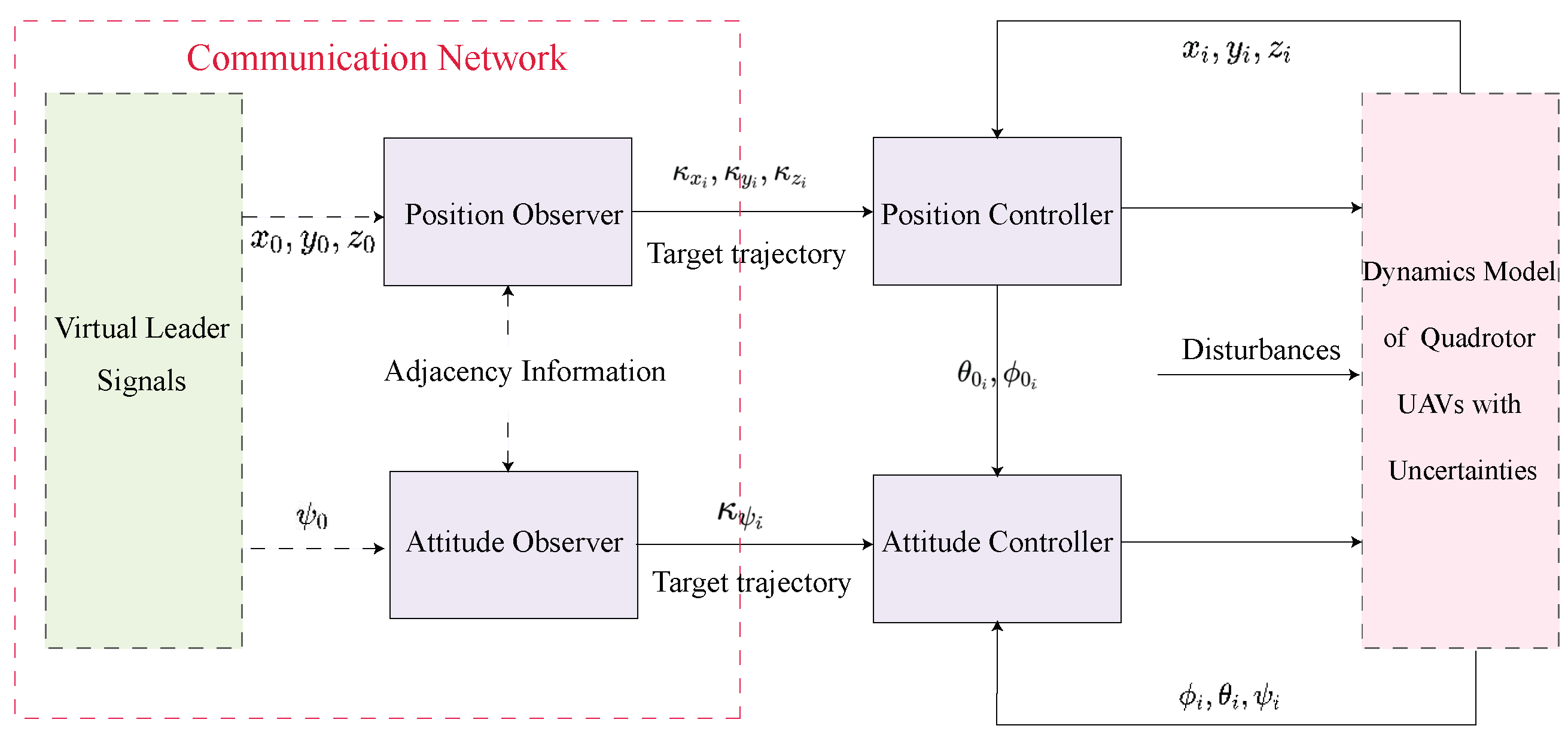
A distributed adaptive velocity observer, integrated with the predefined-time control scheme, is proposed to generate an online estimation of the leader’s information based on uncertain multi-UAV systems. Consequently, the developed neural network-based predefined-time control strategy can fully guarantee asymptotic convergence to the desired geometric position pattern while also achieving complete attitude synchronization.

(2).

A sliding-mode variable within the predefined-time framework is introduced to design the neural network-based intelligent formation algorithm for multi-UAV systems with uncertain dynamics and external disturbances. This approach results in a predefined-time formation strategy with faster convergence speed, higher accuracy, and better robustness compared to most existing schemes proposed in Refs. [29,30].

(3).

An RBF neural network technique, with universal approximation and learning capabilities, is effectively applied to implement the predefined-time formation control scheme, which consists of a translational motion controller and a rotational motion controller. This approach can effectively handle uncertain system models and external disturbances, in contrast to most existing formation control schemes reported in recent works [31,32].

The remainder of this article is organized as follows. Section 2 provides the preliminaries on communication topology, predefined-time stability, and the RBF neural network. Section 3 presents the problem formulation, including the motion model and control objectives of multi-quadrotor UAVs. In Section 4, the designed neural network-based predefined-time control strategy, consisting of the translational motion controller and rotational motion controller, along with convergence analysis, is discussed in detail. Section 5 verifies the feasibility of the developed control strategy through numerical simulations. Finally, the paper concludes in Section 6.

Notation 1.

The superscript “^⊤” indicates the transpose of a matrix or vector. Consider a vector $x={\left(x_1,x_2,\dots ,x_n\right)}^{\top }$. The expression $x^{\circ \alpha }$ denotes an element-wise exponentiation operation performed on the vector x, expressed as $x^{\circ \alpha }={\left(x_1^{\alpha },x_2^{\alpha },\dots ,x_n^{\alpha }\right)}^{\top }$. We define the vector ${\mathcal{S}}^{\wp }\left(x\right)$ as ${\mathcal{S}}^{\wp }\left(x\right)={\left(\mathrm{sgn}\left(x_1\right)|x_1{|}^{\wp },\mathrm{sgn}\left(x_2\right)|x_2{|}^{\wp },\dots ,\mathrm{sgn}\left(x_n\right){\left|x_n\right|}^{\wp }\right)}^{\top }$, where $\mathrm{sgn}(·)$ represents the signum function. For vectors $x={[x_1,x_2,\dots ,x_n]}^{\top }\in {\mathbb{R}}^n$ and $k={[k_1,k_2,\dots ,k_n]}^{\top }\in {\mathbb{R}}^n$, the notation $\left|x\right|<\left|k\right|$ implies that $|x_i|<|k_i|$, $i=(1,\dots ,n)$. Additionally, given the vector $q_i\in {\mathbb{R}}^p$, where $i=1,\dots ,n$, we define $q={(q_1^{\top },q_2^{\top },\dots ,q_n^{\top })}^{\top }\in {\mathbb{R}}^{np}$. For any symmetric matrix X, ${\lambda }_{min}\left(X\right)$ denotes the smallest eigenvalue of X. Furthermore, $I_n$ and $0_n$ denote the n-dimensional column vectors where all elements are equal to 1 and 0, respectively. The symbol ⊗ represents the Kronecker product.

2. Preliminaries

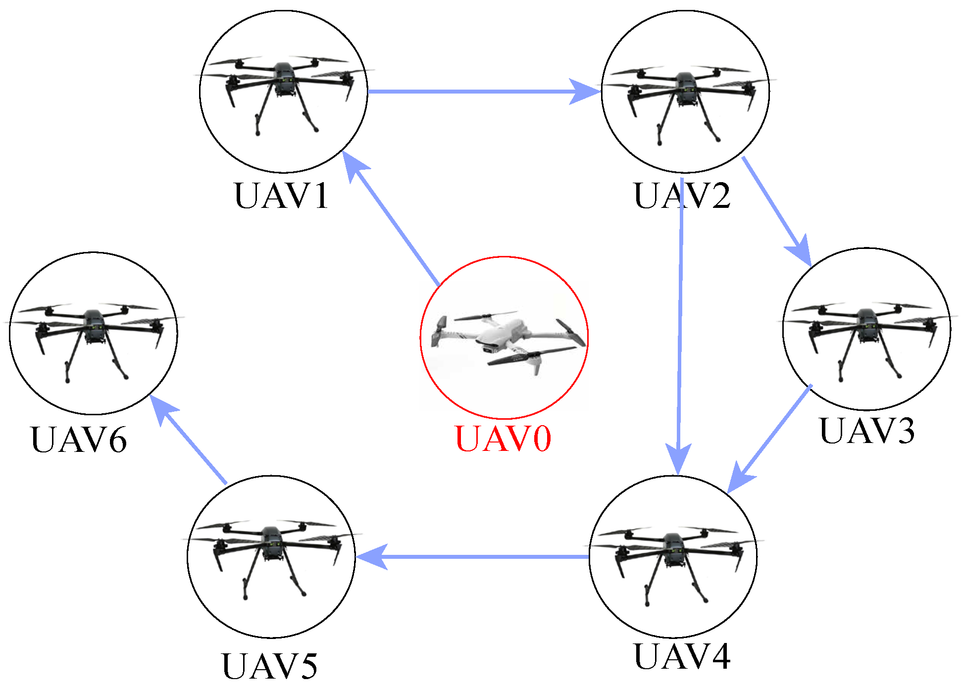
2.1. Communication Topology

The communication network of n quadrotor UAVs is represented by a topology graph $\mathcal{G}=(\mathcal{V},\mathcal{E},\mathcal{A})$, where $\mathcal{V}=\{1,2,\dots ,n\}$ denotes the set of nodes, each representing an individual UAV. The set $\mathcal{E}\subset \mathcal{V}\times \mathcal{V}$ represents the interconnections between the nodes, indicating the communication links between the UAVs. To describe the communication dynamics within the network, the Laplacian matrix $\mathcal{L}={\left[l_{ij}\right]}_{n\times n}\in {\mathbb{R}}^{n\times n}$ is introduced, which captures the overall interaction behavior among the UAVs. Additionally, the adjacency matrix $\mathcal{A}={\left[a_{ij}\right]}_{n\times n}\in {\mathbb{R}}^{n\times n}$ reflects the connectivity structure of the network, with each element $a_{ij}$ indicating whether a communication link exists between UAVs i and j.

Specifically, if $(i,j)\notin \mathcal{E}$, then the adjacency matrix can be defined as $a_{ij}=0$. Consequently, the Laplacian matrix is computed as $l_{ij}=-a_{ij}$ for $i\ne j$, while $l_{ii}={\sum }_{j=1}^n{a}_{ij}$. It is important to note that a quadrotor UAV does not communicate with itself, and thus, $a_{ii}=0$ for all $i\in \mathcal{V}$.

In the context of a leader–follower framework, we introduce a diagonal matrix $\mathcal{B}=\mathrm{diag}\left\{b_1,b_2,\dots ,b_n\right\}$ to characterize the information exchange between the leader and its followers. Here, $b_i>0$ indicates that follower i receives information from the leader, while $b_i=0$ signifies the absence of such communication.

As articulated in the literature [33], the following assumption holds:

Assumption 1.

In scenarios where a virtual dynamic leader follows an anticipated time-fluctuating flight path for quadrotor UAVs, it is crucial to maintain a connection between at least one agent and this leader. This ensures that every team’s communication graph retains a directed spanning tree structure, facilitating cohesive formation and control.

2.2. Predefined-Time Stability

Lemma 1

([34]). Consider the nonlinear system

$$\dot{x}=f\left(x\right),x\left(0\right)=x_0,$$

(1)

where $x\in {\mathbb{R}}^n$ is the system state. The function $f:{\mathbb{R}}^n\to {\mathbb{R}}^n$ is assumed to be nonlinear and continuous and satisfies $f\left(0\right)=0$. Suppose there exists a continuous function $V:{\mathbb{R}}^n\to {\mathbb{R}}_{+}\cup \left\{0\right\}$ that satisfies the following conditions: $V\left(x\right)\to +\infty$ as $\parallel x\parallel \to +\infty$; $V\left(x\right)=0$ if and only if $x=0$; and for all $x\in {\mathbb{R}}^n$, there exist constants ${\varrho }_1,{\varrho }_2>0$, $0<{\phi }_1<1$, and ${\phi }_2>1$ such that

$$\dot{V}\left(x\right)\le -\sum _{i=1}^2{\varrho }_i{V}^{{\phi }_i}\left(x\right).$$

(2)

Under these conditions, the origin $x=0$ of system (1) is fixed-time stable, and the settling time satisfies

$$T^{\ast }={\displaystyle \frac{{\left(\frac{{\varrho }_1}{{\varrho }_2}\right)}^{\frac{1-{\phi }_1}{{\phi }_2-{\phi }_1}}}{{\varrho }_1({\phi }_2-{\phi }_1)}}\prod _{i=1}^2\Gamma \left({\displaystyle \frac{|1-{\phi }_i|}{{\phi }_2-{\phi }_1}}\right),$$

(3)

where $\Gamma \left(x\right)$ is the gamma function defined as $\Gamma \left(x\right)={\int }_0^{\infty }exp(-t)t^{x-1}dt$.

Moreover, if there exist constants ${\varrho }_1,{\varrho }_2>0$, $0<{\phi }_1<1$, and ${\phi }_2>1$ such that

$$\dot{V}\left(x\right)\le -{\displaystyle \frac{T^{\ast }}{T_f}}\sum _{i=1}^2{\varrho }_i{V}^{{\phi }_i}\left(x\right),$$

(4)

then the origin of (1) is predefined-time stable, and $T_f$ is a predefined time.

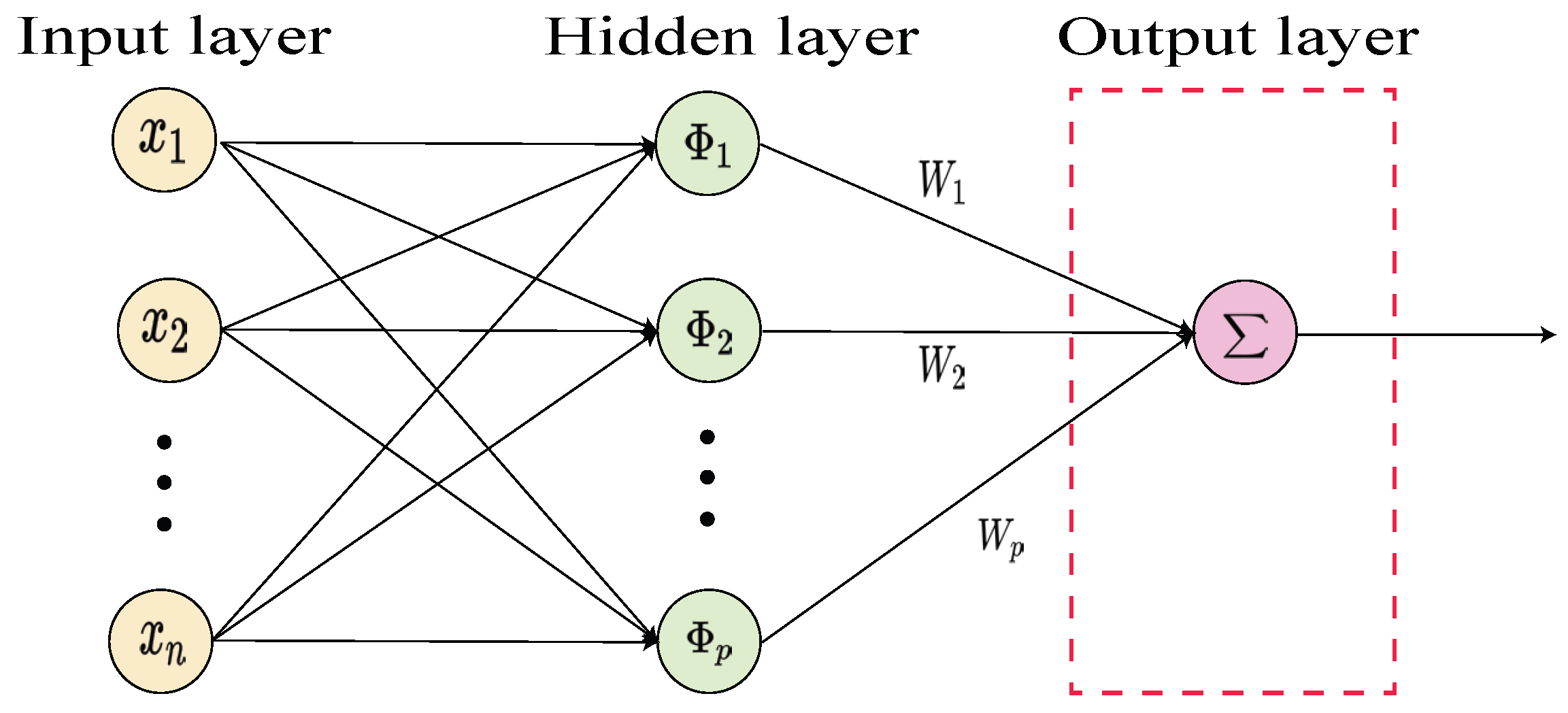
2.3. RBF Neural Network

The RBF neural network [35] serves to estimate the unidentified component of the controlled target $f\left(x\right):{\mathbb{R}}^m\to {\mathbb{R}}^n$ within a specified scope $\mathsf{\Omega }$:

$$f\left(x\right)=W^{\ast \top }\mathsf{\Phi }\left(x\right)+ϵ\left(x\right),$$

(5)

where $W^{\ast }\in {\mathbb{R}}^{p\times n}$ represents the ideal RBF neural network weighted matrix, and $ϵ\left(x\right)\in {\mathbb{R}}^n$ indicates the bounded estimation discrepancy, which satisfies $∥ϵ∥\le \delta$, with $\delta >0$ being a constant that defines the error limit. $\mathsf{\Phi }\left(x\right)={[{\mathsf{\Phi }}_1\left(x\right),\dots ,{\mathsf{\Phi }}_p\left(x\right)]}^{\top }\in {\mathbb{R}}^p$ is the RBF vector, defined as

$${\mathsf{\Phi }}_i\left(x\right)=exp\left(-{\displaystyle \frac{{(x-{\mu }_i)}^{\top }(x-{\mu }_i)}{b_i^2}}\right),i=1,\dots ,p,$$

where ${\mu }_i={[{\mu }_{i,1},\dots ,{\mu }_{i,n}]}^{\top }\in {\mathbb{R}}^n$ denotes the center of the receptive field, and $b_i={[b_{i,1},\dots ,b_{i,n}]}^{\top }\in {\mathbb{R}}^n$ is the width of the RBF. The RBF neural network structure is shown in Figure 1.

3. Problem Formulation

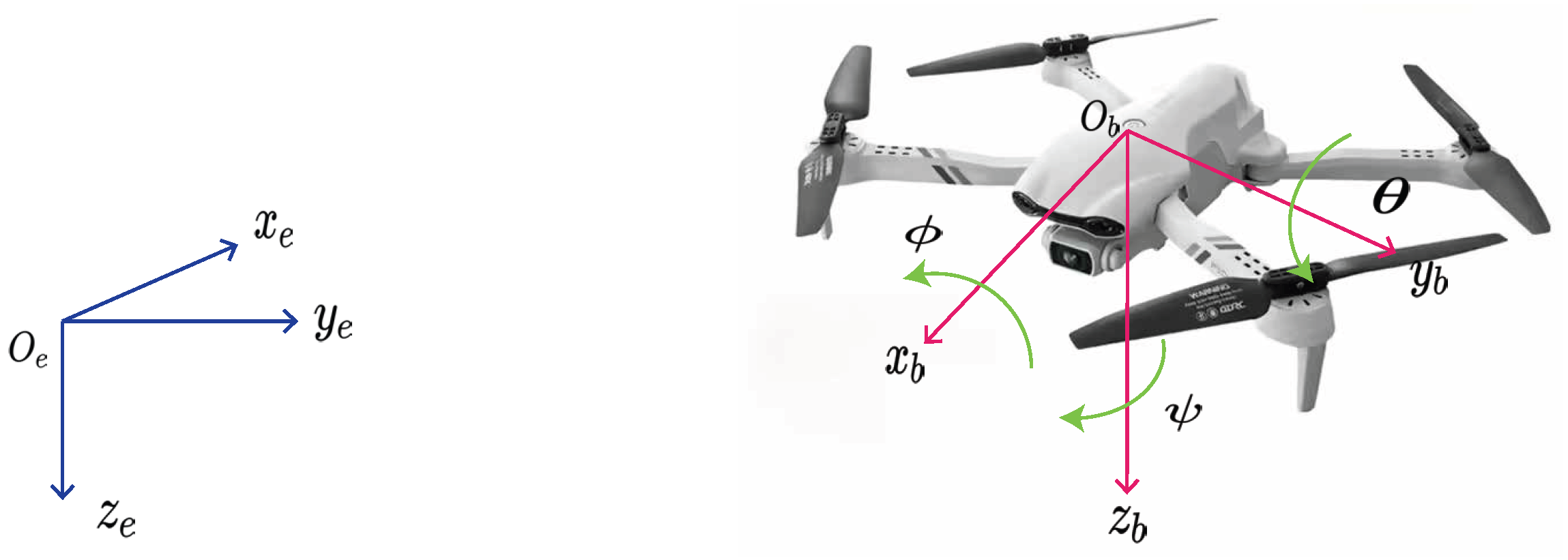
3.1. Quadrotor UAV Model

Regarding the body dynamics, the quadrotor’s mathematical model is commonly derived using two coordinate systems [36]: the airframe frame, $f_b=\left\{O_b,x_b,y_b,z_b\right\}$, and the inertial (or world) frame, $f_e=\left\{O_e,x_e,y_e,z_e\right\}$, as depicted in Figure 2.

A quadrotor UAV is a typical underactuated system. During flight operations, it experiences six types of motion: vertical motion, forward/backward motion, lateral motion, and three rotational motions—roll, yaw, and pitch. However, the system is controlled by only four inputs, as the four motors generate both lifting force and rotational torque in three directions. By adjusting the rotation of the motors, the attitude of the quadrotor UAV can be controlled.

The quadrotor UAV can be separated into two subsystems: the position subsystem and the attitude subsystem, also referred to as the linear motion and angular motion subsystems, respectively. Typically, the control loop for the position subsystem is referred to as the outer loop, while the control loop for the attitude subsystem is known as the inner loop.

To compute the second-order derivative of the Euler angles, the angular acceleration in the body coordinate system must be transformed into the inertial coordinate system using a rotation matrix. However, during this transformation, the sine and cosine terms of the Euler angles become coupled with the control inputs, introducing nonlinear effects. The following assumptions are made to facilitate the subsequent derivation:

Assumption 2.

It is assumed that the Euler angles remain sufficiently small [37]. Furthermore, it is assumed that measurements of the Euler angles and linear positions are available, and measurement noise is neglected.

Define the position state vector of each quadrotor UAV relative to the inertial frame as $q_i={[x_i,y_i,z_i]}^{\top }$ for $i=1,2,\dots ,n$. Additionally, let ${\mathbf{q}}_i={[{\varphi }_i,{\theta }_i,{\psi }_i]}^{\top }$ denote the attitude state vector of each quadrotor UAV within the same inertial coordinate frame, where ${\varphi }_i$, ${\theta }_i$, and ${\psi }_i$ correspond to the roll, pitch, and yaw angles, respectively. The dynamics model of the i-th quadrotor UAV can be described as [38]

$$\begin{array}{c}\hfill \left\{\begin{array}{cc}{\ddot{x}}_i=\hfill & U_{x_i}-{\displaystyle \frac{Q_{x_i}{\dot{x}}_i}{m_i}}+{\Delta }_{x_i}(x_i,{\dot{x}}_i)+{\delta }_{x_i},\hfill \\ {\ddot{y}}_i=\hfill & U_{y_i}-{\displaystyle \frac{Q_{y_i}{\dot{y}}_i}{m_i}}+{\Delta }_{y_i}(y_i,{\dot{y}}_i)+{\delta }_{y_i},\hfill \\ {\ddot{z}}_i=\hfill & U_{z_i}-{\displaystyle \frac{Q_{z_i}{\dot{z}}_i}{m_i}}-g+{\Delta }_{z_i}(z_i,{\dot{z}}_i)+{\delta }_{z_i},\hfill \\ {\ddot{\varphi }}_i=\hfill & U_{{\varphi }_i}-{\displaystyle \frac{Q_{{\varphi }_i}{\dot{\varphi }}_i{l}_i}{I_{x_i}}}+{\Delta }_{{\varphi }_i}({\varphi }_i,{\dot{\varphi }}_i)+{\delta }_{{\varphi }_i},\hfill \\ {\ddot{\theta }}_i=\hfill & U_{{\theta }_i}-{\displaystyle \frac{Q_{{\theta }_i}{\dot{\theta }}_i{l}_i}{I_{y_i}}}+{\Delta }_{{\theta }_i}({\theta }_i,{\dot{\theta }}_i)+{\delta }_{{\theta }_i},\hfill \\ {\ddot{\psi }}_i=\hfill & U_{{\psi }_i}-{\displaystyle \frac{Q_{{\psi }_i}{\dot{\psi }}_i{l}_i}{I_{z_i}}}+{\Delta }_{{\psi }_i}({\psi }_i,{\dot{\psi }}_i)+{\delta }_{{\psi }_i},\hfill \end{array}\right.\end{array}$$

(6)

where $U_{{.}_i}$ ($.=\varphi ,\theta ,\psi ,t$) represents the actual control inputs generated by the four rotors, with $U_{t_i}$ corresponding to $U_{{.}_i}$ ($.=x,y,z$). Additionally, $U_{{.}_i}$ ($.=\varphi ,\theta ,\psi ,t$) is defined as

$$\left[\begin{array}{c}{U}_{t_i}\\ U_{{\varphi }_i}\\ U_{{\theta }_i}\\ U_{{\psi }_i}\end{array}\right]=\left[\begin{array}{cccc}{b}_1& b_1& b_1& b_1\\ -b_1& 0& b_1& 0\\ 0& -b_1& 0& b_1\\ b_2& -b_2& b_2& -b_2\end{array}\right]\left[\begin{array}{c}{\mathsf{\Omega }}_{i1}^2\\ {\mathsf{\Omega }}_{i2}^2\\ {\mathsf{\Omega }}_{i3}^2\\ {\mathsf{\Omega }}_{i4}^2\end{array}\right],$$

(7)

where $b_1$ is the lift coefficient, $b_2$ is the reverse moment coefficient, and ${\mathsf{\Omega }}_{i.}(.=1,2,3,4)$ represents the rotational speeds of the four propellers. Furthermore, $U_{{.}_i}$ ($.=x,y,z$) denotes the virtual control input components for the horizontal, vertical, and altitude, respectively, and it satisfies

$$\begin{array}{c}\hfill \left\{\begin{array}{cc}{U}_{x_i}\hfill & =\left(cos\left({\varphi }_i\right)sin\left({\theta }_i\right)cos\left({\psi }_i\right)+sin\left({\varphi }_i\right)sin\left({\psi }_i\right)\right)U_{t_i},\hfill \\ U_{y_i}\hfill & =\left(cos\left({\varphi }_i\right)sin\left({\theta }_i\right)cos\left({\psi }_i\right)-sin\left({\varphi }_i\right)sin\left({\psi }_i\right)\right)U_{t_i},\hfill \\ U_{z_i}\hfill & =\left(cos\left({\varphi }_i\right)cos\left({\theta }_i\right)\right)U_{t_i}.\hfill \end{array}\right.\end{array}$$

(8)

The other system variables are defined as follows: $l_i$ represents the radius length, while $I_{x_i}$, $I_{y_i}$, and $I_{z_i}$ refer to the moments of inertia about the x-, y-, and z-axes, respectively. The drag factors are denoted by $Q_{{.}_i}$ ($.=x,y,z,\varphi ,\theta ,\psi$). Additionally, ${\Delta }_{{.}_i}$ ($.=x,y,z,\varphi ,\theta ,\psi$) is a vector ${[{\Delta }_{q_i},{\Delta }_{{\mathbf{q}}_i}]}^{\top }$, which represents the bounded uncertainties in the model. Finally, ${\delta }_{{.}_i}$ ($.=x,y,z,\varphi ,\theta ,\psi$) is another vector ${[{\delta }_{q_i},{\delta }_{{\mathbf{q}}_i}]}^{\top }$, representing the bounded external disturbances.

3.2. Control Objective

This control design is divided into two main components. The first component addresses the position subsystem of the UAVs. Initially, we formulate variables related to the position to estimate the desired state of each UAV within the multi-UAV systems. After that, we develop a predefined-time neural adaptive formation position controller. The second component focuses on the UAV attitude subsystem. Initially, we design angle-related variables to estimate the objective information. Following this, we construct a predefined-time neural adaptive controller specifically for attitude synchronization. The overall framework of the control protocol for the quadrotor UAV cluster is depicted in Figure 3.

The primary objective of the position subsystem is to develop a thoroughly distributed predefined-time position control procedure, enabling multi-UAV systems to establish and maintain a rigid formation structure within whichever predefined-time interval $T_p>0$, i.e.,

$$\left\{\begin{array}{c}\begin{array}{cccc}\hfill \underset{t\to T_p^{-}}{lim}(q_i\left(t\right)-q_0\left(t\right))& =d_i,\hfill & \hfill & t\in [0,T_p)\hfill \\ \hfill \underset{t\to T_p^{-}}{lim}({\dot{q}}_i\left(t\right)-{\dot{q}}_0\left(t\right))& =0,\hfill & \hfill & t\in [0,T_p)\hfill \end{array}\hfill \end{array}\right.$$

(9)

where $d_i\in {\mathbb{R}}^3$ represents the formation distance, and $q_0,{\dot{q}}_0\in {\mathbb{R}}^3$ are the leader’s position and velocity, respectively. The leader of the multi-UAV system is governed by

$${\ddot{q}}_0=f(q_0,{\dot{q}}_0),$$

(10)

It is assumed that the virtual leader moves at a constant velocity, i.e., ${\dot{q}}_0=\mathcal{K}$, where $\mathcal{K}$ is a constant.

The main goal of the attitude subsystem is to develop control protocols for attitude synchronization, ensuring that the actual attitude state accurately follows the desired command information within a predefined-time interval $T_a>0$, that is,

$$\begin{array}{cccc}\hfill \underset{t\to T_a^{-}}{lim}({\psi }_i\left(t\right)-{\psi }_0\left(t\right))& =0,\hfill & \hfill & t\in [0,T_a)\hfill \end{array}$$

(11)

where ${\psi }_0$ is a constant representing the leader’s yaw angle.

4. Predefined-Time Motion Control for Translational Systems

4.1. Translational Motion Controller

Based on Equation (6), the position subsystem for the i-th quadrotor UAV can be represented by the following equations:

$$\begin{array}{ccc}\hfill {\ddot{q}}_i& =& U_{q_i}+F_{q_i}+{\mathsf{\Theta }}_{q_i},\hfill \end{array}$$

(12)

where ${\mathsf{\Theta }}_{q_i}$ signifies the lumped uncertainties, which, along with $U_{q_i}$ and $F_{q_i}$, can be expressed as follows:

$$\begin{array}{c}\hfill \left\{\begin{array}{cc}\hfill U_{q_i}& ={[U_{x_i},U_{y_i},U_{z_i}]}^{\top },\hfill \\ \hfill {\mathsf{\Theta }}_{q_i}& ={\Delta }_{q_i}+{\delta }_{q_i},\hfill \\ \hfill F_{q_i}& ={\left[-{\displaystyle \frac{Q_{x_i}{\dot{x}}_i}{m_i}},-{\displaystyle \frac{Q_{y_i}{\dot{y}}_i}{m_i}},-{\displaystyle \frac{Q_{z_i}{\dot{z}}_i}{m_i}}-g\right]}^{\top }.\hfill \end{array}\right.\end{array}$$

(13)

Now, we define the position formation tracking errors for the i-th quadrotor UAV as follows:

$$\begin{array}{ccc}\hfill e_{q_i}& =& \sum _{j=1}^N{a}_{ij}\left(\left(q_i-d_i\right)-\left(q_j-d_j\right)\right)+b_i(q_i-q_0-d_i).\hfill \end{array}$$

(14)

Let $\overline{\mathcal{H}}=\mathcal{H}\otimes I_3$, with $\mathcal{H}=\mathcal{L}+\mathcal{B}$. According to matrix theory, error variables in Equation (14) can be succinctly represented as

$$\begin{array}{ccc}\hfill E_q& =& \overline{\mathcal{H}}(Q-D-Q_0).\hfill \end{array}$$

(15)

where $E_q={\left(e_{q_1}^{\top },e_{q_2}^{\top },\dots ,e_{q_n}^{\top }\right)}^{\top }$, $Q={\left(q_1^{\top },q_2^{\top },\dots ,q_n^{\top }\right)}^{\top }$, and $Q_0=1_n\otimes q_0$, while the vector $D={\left(d_1^{\top },d_2^{\top },\dots ,d_n^{\top }\right)}^{\top }$.

Based on the RBF neural network algorithm mentioned above, the uncertain nonlinear component ${\mathsf{\Theta }}_{q_i}$ is approximated as follows:

$${\mathsf{\Theta }}_{q_i}\left(x_{q_i}\right)={W_{q_i}^{\ast }}^{\top }{\mathsf{\Phi }}_{q_i}\left(x_{q_i}\right)+{ϵ}_{q_i},$$

(16)

where $x_{q_i}={[e_{q_i},{\dot{e}}_{q_i}]}^{\top }$, and ${ϵ}_{q_i}$ denotes the bounded approximation error. Define $\left|{ϵ}_{q_i}\right|\le {ϵ}_{{q_i}_{max}}$ for ${ϵ}_{{q_i}_{max}}>0$. $W_{q_i}^{\ast }={[W_{q_{i,1}}^{\ast },W_{q_{i,2}}^{\ast },W_{q_{i,3}}^{\ast }]}^{\top }$, ${\mathsf{\Phi }}_{q_i}={[{\mathsf{\Phi }}_{q_{i,1}},{\mathsf{\Phi }}_{q_{i,2}},{\mathsf{\Phi }}_{q_{i,3}}]}^{\top }$, and ${\mathsf{\Phi }}_{q_{i,j}}={[{\mathsf{\Phi }}_{q_{i,j,1}},\dots ,{\mathsf{\Phi }}_{q_{i,j,l}}]}^{\top }$ is the RBF vector, where $(j=1,2,3)$, and l is the neural network node number. ${\mathsf{\Phi }}_{q_{i,j,k}}$ is often selected as

$${\mathsf{\Phi }}_{q_{i,j,k}}\left(x_{q_i}\right)=exp\left({\displaystyle \frac{-{(x_{q_{i,j}}-{\mu }_{q_{i,j,k}})}^{\top }(x_{q_{i,j}}-{\mu }_{q_{i,j,k}})}{b_{q_{i,j,k}}^2}}\right),$$

(17)

where $k=(1,\dots ,l)$, $x_{q_{i,j}}={[e_{q_{i,j}},{\dot{e}}_{q_{i,j}}]}^{\top }$, ${\mu }_{q_{i,j}}={[{\mu }_{q_{i,j,1}},\dots ,{\mu }_{q_{i,j,l}}]}^{\top }$ is the central parameter of each neuron in the hidden layer, and $b_{q_{i,j}}=[b_{q_{i,j,1}},\dots ,b_{q_{i,j,l}}]$ is the width of the RBF. Define the weighted estimation error as ${\tilde{W}}_{q_{i,j}}={\widehat{W}}_{q_{i,j}}-W_{q_{i,j}}^{\ast }$, where ${\widehat{W}}_{q_{i,j}}$ represents the estimated value of the optimal weight $W_{q_{i,j}}^{\ast }$. The corresponding adaptive law is formulated as

$${\dot{\widehat{W}}}_{q_{i,j}}=P_{q_{i,j}}{\mathsf{\Phi }}_{q_{i,j}}{s}_{q_{i,j}},$$

(18)

where $P_{q_{i,j}}$ denotes a symmetric positive definite matrix, and $s_{q_{i,j}}$ is a sliding surface, which will be defined further.

To achieve predefined-time formation control, a velocity observation control strategy is employed. If the i-th follower can obtain the leader’s information, we set $b_i>0$; otherwise, $b_i=0$, as only a limited subset of formation members have access to the leader’s information [39]. Consequently, an auxiliary variable, ${\hslash }_{q_i}$, is introduced and defined as

$${\hslash }_{q_i}=\sum _{j=1}^N{a}_{ij}({\widehat{v}}_i-{\widehat{v}}_j)+b_i({\widehat{v}}_i-{\dot{q}}_0),$$

(19)

where ${\widehat{v}}_i$ represents the estimation of ${\dot{q}}_0$ and is formally defined as

$${\dot{\widehat{v}}}_i=-{\displaystyle \frac{{\chi }_{q_1}}{T_1}}\left({\mathcal{S}}^{{\alpha }_1}\left({\hslash }_{q_i}\right)+{\mathcal{S}}^{{\alpha }_2}\left({\hslash }_{q_i}\right)\right),$$

(20)

where $0<{\alpha }_1<1<{\alpha }_2$, ${\chi }_{q_1}$ denotes the observer gain to be determined subsequently, and $T_1>0$ represents the predefined time for observation. According to matrix theory, the auxiliary variable ${\hslash }_q$ can be written as ${\hslash }_q=\overline{\mathcal{H}}{\xi }_q$, where ${\xi }_q={({\xi }_{q_1}^{\top },{\xi }_{q_2}^{\top },\dots ,{\xi }_{q_n}^{\top })}^{\top }$ with ${\xi }_{q_i}={\widehat{v}}_i-v_0$.

Subsequently, a predefined-time terminal sliding-mode variable is formulated as

$$s_{q_i}={\dot{q}}_i-{\widehat{v}}_i+{\displaystyle \frac{{\chi }_{q_3}}{T_3}}\left(\mathcal{S}{\left(e_{q_i}\right)}^{{\gamma }_1}+\mathcal{S}{\left(e_{q_i}\right)}^{{\gamma }_2}\right),$$

(21)

where $0<{\gamma }_1<1<{\gamma }_2$, $T_3>0$ is the predefined time for sliding, ${\chi }_{q_3}$ is the position control gain to be designed later, and the time derivative of $s_{q_i}$ is

$${\dot{s}}_{q_i}={\ddot{q}}_i-{\dot{\widehat{v}}}_i+{\displaystyle \frac{{\chi }_{q_3}}{T_3}}\left({\gamma }_1\mathrm{diag}\left({\left|e_{q_i}\right|}^{{\gamma }_1-1}\right){\dot{e}}_{q_i}+{\gamma }_2\mathrm{diag}\left({\left|e_{q_i}\right|}^{{\gamma }_2-1}\right){\dot{e}}_{q_i}\right).$$

(22)

Building upon the dynamics equations of the position subsystem for the i-th quadrotor UAV, as delineated in Equation (12), in conjunction with the uncertain nonlinear component estimated via the RBF neural network algorithm presented in Equation (16), the expression for ${\dot{s}}_{q_i}$ in Equation (22) can be reformulated as follows:

$$\begin{array}{cc}\hfill {\dot{s}}_{q_i}=& U_{q_i}+F_{q_i}+{W_{q_i}^{\ast }}^{\top }{\mathsf{\Phi }}_{q_i}\left(x_{q_i}\right)+{ϵ}_{q_i}-{\dot{\widehat{v}}}_i\hfill \\ \hfill & +{\displaystyle \frac{{\chi }_{q_3}}{T_3}}\left({\gamma }_1\mathrm{diag}\left({\left|e_{q_i}\right|}^{{\gamma }_1-1}\right){\dot{e}}_{q_i}+{\gamma }_2\mathrm{diag}\left({\left|e_{q_i}\right|}^{{\gamma }_2-1}\right){\dot{e}}_{q_i}\right).\hfill \end{array}$$

(23)

To guarantee the convergence of the position subsystem within a predefined time, we propose a predefined-time adaptive controller integrating the RBF neural network, formulated as follows:

$$\begin{array}{cc}\hfill U_{q_i}=& -{\widehat{W}}_{q_i}^{\top }{\mathsf{\Phi }}_{q_i}-{ϵ}_{{\mathrm{q}}_{\mathrm{i}}max}\mathrm{sgn}\left(s_{q_i}\right)-{\vartheta }_{q_i}\mathrm{sgn}\left(s_{q_i}\right)-F_{q_i}+{\dot{\widehat{v}}}_i\hfill \\ \hfill & -{\displaystyle \frac{{\chi }_{q_3}}{T_3}}\left({\gamma }_1\mathrm{diag}\left({\left|e_{q_i}\right|}^{{\gamma }_1-1}\right){\dot{e}}_{q_i}+{\gamma }_2\mathrm{diag}\left({\left|e_{q_i}\right|}^{{\gamma }_2-1}\right){\dot{e}}_{q_i}\right)\hfill \\ \hfill & -{\displaystyle \frac{{\chi }_{q_2}}{T_2}}\left(\mathcal{S}{\left(s_{q_i}\right)}^{{\beta }_1}+\mathcal{S}{\left(s_{q_i}\right)}^{{\beta }_2}\right),\hfill \end{array}$$

(24)

where $0<{\beta }_1<1<{\beta }_2$, and ${\chi }_{q_2}$ denotes the position control gain to be determined subsequently, while $T_2>0$ signifies the predefined time for reaching. Additionally, ${\vartheta }_{q_i}$ is defined as a diagonal matrix whose elements fulfill the condition ${\vartheta }_{q_{i,j}}\ge {\tilde{W}}_{q_{i,j}}^{\top }{\mathsf{\Phi }}_{q_{i,j}}$.

Theorem 1.

Assuming that Assumption 1 holds, the observer (20) can estimate the desired velocity of the i-th follower within the predefined-time interval $T_1$. Then, using the neural adaptive controller (24) and the terminal sliding-mode variable (21), the predefined-time formation of the position subsystem can be achieved within the predefined time $T_1+T_2+T_3$. This depends on the proper selection of the control parameters ${\chi }_{q_1},{\chi }_{q_2}$, and ${\chi }_{q_3}$, as follows:

$$\begin{array}{cc}\hfill & {\chi }_{q_1}={\displaystyle \frac{1}{{\lambda }_{min}\left(\mathcal{H}\right)({\alpha }_2-{\alpha }_1)}}{\left(3n\right)}^{{\displaystyle \frac{({\alpha }_2-1)(1-{\alpha }_1)}{2({\alpha }_2-{\alpha }_1)}}}\prod _{i=1}^2\Gamma \left({\displaystyle \frac{|1-{\alpha }_i|}{{\alpha }_2-{\alpha }_1}}\right),\hfill \\ \hfill & {\chi }_{q_2}={\displaystyle \frac{1}{({\beta }_2-{\beta }_1)}}{\left(3n\right)}^{{\displaystyle \frac{({\beta }_2-1)(1-{\beta }_1)}{2({\beta }_2-{\beta }_1)}}}\prod _{i=1}^2\Gamma \left({\displaystyle \frac{|1-{\beta }_i|}{{\beta }_2-{\beta }_1}}\right),\hfill \\ \hfill & {\chi }_{q_3}={\displaystyle \frac{1}{{\lambda }_{min}\left(\mathcal{H}\right)({\gamma }_2-{\gamma }_1)}}{\left(3n\right)}^{{\displaystyle \frac{({\gamma }_2-1)(1-{\gamma }_1)}{2({\gamma }_2-{\gamma }_1)}}}\prod _{i=1}^2\Gamma \left({\displaystyle \frac{|1-{\gamma }_i|}{{\gamma }_2-{\gamma }_1}}\right).\hfill \end{array}$$

(25)

4.2. Translational Motion Stability Analysis

Proof. 

The proof is organized into two primary steps.

Step 1: We will establish that the position subsystem defined in Equation (6) can converge to the sliding surface $s_{q_{i,j}}=0$ within the predefined-time interval $T_1+T_2$.

Initially, consider the Lyapunov function given by

$$V_{q_1}\left(t\right)={\displaystyle \frac{1}{2}}{\xi }_q^{\top }\overline{\mathcal{H}}{\xi }_q.$$

(26)

The time derivative of $V_{q_1}\left(t\right)$ along the trajectories of ${\xi }_q$ is expressed as

$$\begin{array}{cc}\hfill {\dot{V}}_{q_1}\left(t\right)& =-{\displaystyle \frac{{\chi }_{q_1}}{T_1}}\left({\xi }_q^{\top }\overline{\mathcal{H}}{\mathcal{S}}^{{\alpha }_1}\left(\overline{\mathcal{H}}{\xi }_q\right)+{\xi }_q^{\top }\overline{\mathcal{H}}{\mathcal{S}}^{{\alpha }_2}\left(\overline{\mathcal{H}}{\xi }_q\right)\right)\hfill \\ \hfill & =-{\displaystyle \frac{{\chi }_{q_1}}{T_1}}\left(\parallel \overline{\mathcal{H}}{\xi }_q{\parallel }_{{\alpha }_1+1}^{{\alpha }_1+1}+{\parallel \overline{\mathcal{H}}{\xi }_q\parallel }_{{\alpha }_2+1}^{{\alpha }_2+1}\right).\hfill \end{array}$$

(27)

Utilizing the condition $0<{\alpha }_1<1<{\alpha }_2$, the following inequality can be derived:

$$\begin{array}{cc}\hfill {\dot{V}}_{q_1}\left(t\right)& \le -{\displaystyle \frac{{\chi }_{q_1}}{T_1}}\parallel \overline{\mathcal{H}}{\xi }_q{\parallel }_2^{{\alpha }_1+1}-{\displaystyle \frac{{\chi }_{q_1}}{T_1}}{\parallel \overline{\mathcal{H}}{\xi }_q\parallel }_2^{{\alpha }_2+1}{\left(3n\right)}^{{\displaystyle \frac{1-{\alpha }_2}{2}}}\hfill \\ \hfill & \le -{\displaystyle \frac{{\chi }_{q_1}}{T_1}}{\left(2{\lambda }_{min}\left(\mathcal{H}\right)V_{q_1}\right)}^{{\displaystyle \frac{{\alpha }_1+1}{2}}}-{\displaystyle \frac{{\chi }_{q_1}}{T_1}}{\left(2{\lambda }_{min}\left(\mathcal{H}\right)V_{q_1}\right)}^{{\displaystyle \frac{{\alpha }_2+1}{2}}}{\left(3n\right)}^{{\displaystyle \frac{1-{\alpha }_2}{2}}}\hfill \\ \hfill & \le -{\displaystyle \frac{{\chi }_{q_1}}{T_1}}\left({\varsigma }_{q_1}{V}_{q_1}^{{\displaystyle \frac{{\alpha }_1+1}{2}}}+{\varsigma }_{q_2}{V}_{q_1}^{{\displaystyle \frac{{\alpha }_2+1}{2}}}\right),\hfill \end{array}$$

(28)

where ${\varsigma }_{q_1}={\left(2{\lambda }_{min}\left(\mathcal{H}\right)\right)}^{{\displaystyle \frac{{\alpha }_1+1}{2}}}$ and ${\varsigma }_{q_2}={\left(2{\lambda }_{min}\left(\mathcal{H}\right)\right)}^{{\displaystyle \frac{{\alpha }_2+1}{2}}}{\left(3n\right)}^{{\displaystyle \frac{1-{\alpha }_2}{2}}}$. The parameter ${\chi }_{q_1}$ is defined as

$${\chi }_{q_1}={\displaystyle \frac{1}{{\lambda }_{min}\left(\mathcal{H}\right)({\alpha }_2-{\alpha }_1)}}{\left(3n\right)}^{{\displaystyle \frac{({\alpha }_2-1)(1-{\alpha }_1)}{2({\alpha }_2-{\alpha }_1)}}}\prod _{i=1}^2\Gamma \left({\displaystyle \frac{|1-{\alpha }_i|}{{\alpha }_2-{\alpha }_1}}\right).$$

(29)

Subsequently, define $V_{q_3}\left(t\right)={\displaystyle \frac{1}{2}}{s}_q^{\top }{s}_q$ and consider the Lyapunov function given by

$$\begin{array}{cc}\hfill V_{q_2}\left(t\right)=& V_{q_3}\left(t\right)+{\displaystyle \frac{1}{2}}\sum _{i=1}^n\sum _{j=1}^{3}Tr\left({\tilde{W}}_{q_{i,j}}^{\top }{P}_{q_{i,j}}^{-1}{\tilde{W}}_{q_{i,j}}\right).\hfill \end{array}$$

(30)

Then, by differentiating $V_{q_2}\left(t\right)$ with respect to time and integrating the predefined-time neural adaptive controller as presented in Equation (24), along with the predefined-time terminal sliding-mode variable specified in Equation (23), we obtain

$$\begin{array}{cc}\hfill {\dot{V}}_{q_2}\left(t\right)=& s_q^{\top }\left({ϵ}_q-\mathrm{sgn}\left(s_q\right){ϵ}_{q_{max}}-{\vartheta }_q\mathrm{sgn}\left(s_q\right)-{\tilde{W}}_q^{\top }{\mathsf{\Phi }}_q\right)\hfill \\ \hfill & -\sum _{i=1}^n\sum _{j=1}^3{\displaystyle \frac{{\chi }_{q_2}}{T_2}}\left({\left|s_{q_{i,j}}\right|}^{{\beta }_1+1}+{\left|s_{q_{i,j}}\right|}^{{\beta }_2+1}\right)+\sum _{i=1}^n\sum _{j=1}^{3}Tr\left({\tilde{W}}_{q_{i,j}}^{\top }{P}_{q_{i,j}}^{-1}{\dot{\tilde{W}}}_{q_{i,j}}\right)\hfill \\ \hfill \le & -\sum _{i=1}^n\sum _{j=1}^3\left|s_{q_{i,j}}\right|\left({ϵ}_{q_{i_{max}}}-{ϵ}_{q_i}\right)-{\displaystyle \frac{{\chi }_{q_2}}{T_2}}\sum _{i=1}^n\sum _{j=1}^3\left({\left|s_{q_{i,j}}\right|}^{{\beta }_1+1}+{\left|s_{q_{i,j}}\right|}^{{\beta }_2+1}\right)\hfill \\ \hfill & -\sum _{i=1}^n\sum _{j=1}^3\left(s_{q_{i,j}}{\tilde{W}}_{q_{i,j}}^{\top }{\mathsf{\Phi }}_{q_{i,j}}\right)+\sum _{i=1}^n\sum _{j=1}^{3}Tr\left({\tilde{W}}_{q_{i,j}}^{\top }{P}_{q_{i,j}}^{-1}{\dot{\tilde{W}}}_{q_{i,j}}\right).\hfill \end{array}$$

(31)

Based on $s_{q_{i,j}}{\widehat{W}}_{q_{i,j}}^{\top }{\mathsf{\Phi }}_{q_{i,j}}=Tr\left({\widehat{W}}_{q_{i,j}}^{\top }{\mathsf{\Phi }}_{q_{i,j}}{s}_{q_{i,j}}\right),$ and by integrating the adaptive law described in Equation (18), it follows that Equation (54) can be further formulated as

$$\begin{array}{cc}\hfill {\dot{V}}_{q_2}\left(t\right)\le & -\sum _{i=1}^n\sum _{j=1}^3\left|s_{q_{i,j}}\right|\left({ϵ}_{q_{i_{max}}}-{ϵ}_{q_i}\right)-{\displaystyle \frac{{\chi }_{q_2}}{T_2}}\sum _{i=1}^n\sum _{j=1}^3\left({\left|s_{q_{i,j}}\right|}^{{\beta }_1+1}+{\left|s_{q_{i,j}}\right|}^{{\beta }_2+1}\right).\hfill \end{array}$$

(32)

According to Equation (32), it follows that ${\dot{V}}_{q_2}\left(t\right)\le 0$, which implies that both $s_q$ and ${\tilde{W}}_q$ are constrained within bounded limits. In the subsequent sections, we will demonstrate that the trajectories of the tracking error variable $E_q$ can be driven toward the sliding-mode surface $s_{q_{i,j}}=0$ within the predefined-time interval $T_1+T_2$. Building upon the preceding results presented in Equations (31) and (32), we can derive the following:

$$\begin{array}{cc}\hfill {\dot{V}}_{q_3}\left(t\right)\le & -{\displaystyle \frac{{\chi }_{q_2}}{T_2}}\sum _{i=1}^n\sum _{j=1}^3\left({\left|s_{q_{i,j}}\right|}^{{\beta }_1+1}+{\left|s_{q_{i,j}}\right|}^{{\beta }_2+1}\right)\hfill \\ \hfill \le & -{\displaystyle \frac{{\chi }_{q_2}}{T_2}}\left({\left(\sum _{i=1}^n\sum _{j=1}^3{s}_{q_{i,j}}^2\right)}^{{\displaystyle \frac{{\beta }_1+1}{2}}}\right)-{\displaystyle \frac{{\chi }_{q_2}}{T_2}}\left({\left(3n\right)}^{{\displaystyle \frac{1-{\beta }_2}{2}}}{\left(\sum _{i=1}^n\sum _{j=1}^3{s}_{q_{i,j}}^2\right)}^{{\displaystyle \frac{{\beta }_2+1}{2}}}\right)\hfill \\ \hfill \le & -{\displaystyle \frac{{\chi }_{q_2}}{T_2}}\left({\varsigma }_{q_3}{\left(V_{q_3}\right)}^{{\displaystyle \frac{{\beta }_1+1}{2}}}+{\varsigma }_{q4}{\left(V_{q_3}\right)}^{{\displaystyle \frac{{\beta }_2+1}{2}}}\right),\hfill \end{array}$$

(33)

where ${\varsigma }_{q_3}=2^{{\displaystyle \frac{{\beta }_1+1}{2}}}$ and ${\varsigma }_{q_4}=2^{{\displaystyle \frac{{\beta }_2+1}{2}}}{\left(3n\right)}^{{\displaystyle \frac{1-{\beta }_2}{2}}}$, and ${\chi }_{q_2}$ satisfies

$$\begin{array}{c}\hfill {\chi }_{q_2}={\displaystyle \frac{1}{({\beta }_2-{\beta }_1)}}{\left(3n\right)}^{{\displaystyle \frac{({\beta }_2-1)(1-{\beta }_1)}{2({\beta }_2-{\beta }_1)}}}\prod _{i=1}^2\Gamma \left({\displaystyle \frac{|1-{\beta }_i|}{{\beta }_2-{\beta }_1}}\right).\end{array}$$

(34)

Thus, based on Lemma 1, the position subsystem of the quadrotor UAVs are adept at attaining the sliding surface $s_{q_{i,j}}=0$ within the predetermined-time interval $T_1+T_2$.

Step 2: It is established that the position subsystem will achieve the desired formation control within the predefined-time interval $T_1+T_2+T_3$.

Based on the condition $s_{q_{i,j}}=0$ for $t>T_1+T_2$ and integrating this with Equation (21), we derive the following result:

$${\dot{q}}_i-{\widehat{v}}_i=-{\displaystyle \frac{{\chi }_{q_3}}{T_3}}\left(\mathcal{S}{\left(e_{q_i}\right)}^{{\gamma }_1}+\mathcal{S}{\left(e_{q_i}\right)}^{{\gamma }_2}\right).$$

(35)

Subsequently, drawing upon the results of the previous derivation, it follows that ${\dot{q}}_0={\widehat{v}}_i$ for $t>T_1$. Consequently, for $t>T_1+T_2$, the time derivative of $E_q$ can be expressed as follows:

$$\dot{E_q}=\overline{\mathcal{H}}(\dot{Q}-{\dot{Q}}_0)=-{\displaystyle \frac{{\chi }_{q_3}}{T_3}}\overline{\mathcal{H}}\left(\mathcal{S}{\left(E_q\right)}^{{\gamma }_1}+\mathcal{S}{\left(E_q\right)}^{{\gamma }_2}\right).$$

(36)

Define the Lyapunov function as follows:

$$V_{q_4}\left(t\right)={\displaystyle \frac{1}{2}}{E}_q^{\top }{E}_q.$$

(37)

By differentiating $V_{q_4}\left(t\right)$ with respect to time and incorporating Equation (36), we obtain

$$\begin{array}{cc}\hfill {\dot{V}}_{q_4}\left(t\right)=& -E_q^{\top }\left({\displaystyle \frac{{\chi }_{q_3}}{T_3}}\overline{\mathcal{H}}\left(\mathcal{S}{\left(E_q\right)}^{{\gamma }_1}+\mathcal{S}{\left(E_q\right)}^{{\gamma }_2}\right)\right)\hfill \\ \hfill \le & -{\displaystyle \frac{{\chi }_{q_3}}{T_3}}{\lambda }_{min}\left(\mathcal{H}\right)\left(E_q^{\top }{E}_q^{\circ {\gamma }_1}+E_q^{\top }{E}_q^{\circ {\gamma }_2}\right)\hfill \\ \hfill \le & -{\displaystyle \frac{{\chi }_{q_3}}{T_3}}{\lambda }_{min}\left(\mathcal{H}\right)2^{{\displaystyle \frac{{\gamma }_1+1}{2}}}{\left({\displaystyle \frac{1}{2}}{E}_q^{\top }{E}_q\right)}^{{\displaystyle \frac{{\gamma }_1+1}{2}}}\hfill \\ & -{\displaystyle \frac{{\chi }_{q_3}}{T_3}}{\lambda }_{min}\left(\mathcal{H}\right)2^{{\displaystyle \frac{{\gamma }_2+1}{2}}}{\left(3n\right)}^{{\displaystyle \frac{1-{\gamma }_2}{2}}}{\left({\displaystyle \frac{1}{2}}{E}_q^{\top }{E}_q\right)}^{{\displaystyle \frac{{\gamma }_2+1}{2}}}\hfill \\ \hfill \le & -{\displaystyle \frac{{\chi }_{q_3}}{T_3}}\left({\varsigma }_{q_5}{V}_{q_4}^{{\displaystyle \frac{{\gamma }_1+1}{2}}}+{\varsigma }_{q_6}{V}_{q_4}^{{\displaystyle \frac{{\gamma }_2+1}{2}}}\right),\hfill \end{array}$$

(38)

where ${\varsigma }_{q_5}={\lambda }_{min}\left(\mathcal{H}\right)2^{{\displaystyle \frac{{\gamma }_1+1}{2}}}$ and ${\varsigma }_{q_6}={\lambda }_{min}\left(\mathcal{H}\right)2^{{\displaystyle \frac{{\gamma }_2+1}{2}}}{\left(3n\right)}^{{\displaystyle \frac{1-{\gamma }_2}{2}}}$, and ${\chi }_{q_3}$ is defined as

$$\begin{array}{cc}\hfill {\chi }_{q_3}& ={\displaystyle \frac{1}{{\lambda }_{min}\left(\mathcal{H}\right)({\gamma }_2-{\gamma }_1)}}{\left(3n\right)}^{{\displaystyle \frac{({\gamma }_2-1)(1-{\gamma }_1)}{2({\gamma }_2-{\gamma }_1)}}}\prod _{i=1}^2\Gamma \left({\displaystyle \frac{|1-{\gamma }_i|}{{\gamma }_2-{\gamma }_1}}\right).\hfill \end{array}$$

(39)

Thus, the error variable $E_q$ asymptotically converges to zero when $t\ge T_p$, where $T_p$ is defined as $T_p=T_1+T_2+T_3$. This convergence indicates that $E_q=\overline{\mathcal{H}}(Q-D-Q_0)=0_{3n}$. Given that $\mathcal{H}$ is positive definite, this relationship further implies that $Q-Q_0=D$. Additionally, for $t\ge T_p$, the condition ${\dot{E}}_q=\overline{\mathcal{H}}(\dot{Q}-{\dot{Q}}_0)=0_{3n}$ necessitates that $\dot{Q}-{\dot{Q}}_0=0_{3n}$. Consequently, the quadrotor-UAV systems achieve and maintain the desired geometric formation shape precisely within the predefined-time interval $T_p$. □

5. Predefined-Time Motion Control for Rotational Systems

5.1. Rotational Motion Controller

Based on Equation (6), the attitude subsystem of the i-th quadrotor UAV can be expressed in the following form:

$$\begin{array}{ccc}\hfill {\ddot{\mathbf{q}}}_i& =& U_{{\mathbf{q}}_i}+F_{{\mathbf{q}}_i}+{\mathsf{\Theta }}_{{\mathbf{q}}_i},\hfill \end{array}$$

(40)

where ${\mathsf{\Theta }}_{{\mathbf{q}}_i}$ encapsulates the lumped uncertainties, which, together with $U_{{\mathbf{q}}_i}$ and $F_{{\mathbf{q}}_i}$, are expressed as follows:

$$\begin{array}{c}\hfill \left\{\begin{array}{cc}\hfill U_{{\mathbf{q}}_i}& ={[U_{{\varphi }_i},U_{{\theta }_i},U_{{\psi }_i}]}^{\top },\hfill \\ \hfill {\mathsf{\Theta }}_{{\mathbf{q}}_i}& ={\Delta }_{{\mathbf{q}}_i}+{\delta }_{{\mathbf{q}}_i},\hfill \\ \hfill F_{{\mathbf{q}}_i}& ={\left[-{\displaystyle \frac{Q_{{\varphi }_i}{\dot{\varphi }}_i{l}_i}{I_{x_i}}},-{\displaystyle \frac{Q_{{\theta }_i}{\dot{\theta }}_i{l}_i}{I_{y_i}}},-{\displaystyle \frac{Q_{{\psi }_i}{\dot{\psi }}_i{l}_i}{I_{z_i}}}\right]}^{\top }.\hfill \end{array}\right.\end{array}$$

(41)

In view of Equations (6) and (8), it becomes evident that the quadrotor UAVs operate as an underactuated system with four inputs, $U_{t_i}$, $U_{{\varphi }_i}$, $U_{{\theta }_i}$, and $U_{{\psi }_i}$, while possessing six outputs: $x_i$, $y_i$, $z_i$, ${\varphi }_i$, ${\theta }_i$, and ${\psi }_i$. Additionally, the state command for the quadrotor UAV’s roll and pitch angles can be derived from the intermediate control variables $U_{x_i}$, $U_{y_i}$, and $U_{z_i}$. Thus, ${\varphi }_{0_i}$ and ${\theta }_{0_i}$ can be solved as follows [40]:

$$\begin{array}{ccc}\hfill {\theta }_{0_i}& =& arcsin\left({\displaystyle \frac{m_i{U}_{x_i}sin\left({\psi }_i\right)-m_i{U}_{y_i}cos\left({\psi }_i\right)}{U_{t_i}}}\right),\hfill \\ \hfill {\varphi }_{0_i}& =& arctan\left({\displaystyle \frac{U_{x_i}cos\left({\psi }_i\right)+U_{y_i}sin\left({\psi }_i\right)}{U_{z_i}}}\right).\hfill \end{array}$$

(42)

The position control subsystem generates objective information about the quadrotor UAV’s orientation in roll and pitch, which is then relayed to the attitude control subsystem. By implementing attitude control laws, precise tracking of these two rotational angles can be accomplished effectively. Specifically, the objective information for the yaw angle of the i-th UAV is symbolized as ${\psi }_0$, typically established beforehand as an extra reference. Subsequently, the yaw angle tracking error variable, along with its time derivative, is defined as follows:

$$\begin{array}{ccc}\hfill e_{{\psi }_i}& =& \sum _{j=1}^n{a}_{ij}({\psi }_i-{\psi }_j)+b_i({\psi }_i-{\psi }_0).\hfill \end{array}$$

(43)

Building upon the previously discussed RBF neural network algorithm, the uncertain nonlinear component ${\mathsf{\Theta }}_{{\psi }_i}$ is approximated as follows:

$${\mathsf{\Theta }}_{{\psi }_i}\left(x_{{\psi }_i}\right)={W_{{\psi }_i}^{\ast }}^{\top }{\mathsf{\Phi }}_{{\psi }_i}\left(x_{{\psi }_i}\right)+{ϵ}_{{\psi }_i},$$

(44)

where $x_{{\psi }_i}={[e_{{\psi }_i},{\dot{e}}_{{\psi }_i}]}^{\top }$, and ${ϵ}_{{\psi }_i}$ represents the bounded approximation error. Define $\left|{ϵ}_{{\psi }_i}\right|\le {ϵ}_{{{\psi }_i}_{max}}$, where ${ϵ}_{{{\psi }_i}_{max}}>0$. The associated adaptive law is expressed as

$${\dot{\widehat{W}}}_{{\psi }_i}=P_{{\psi }_i}{\mathsf{\Phi }}_{{\psi }_i}{s}_{{\psi }_i},$$

(45)

where $P_{{\psi }_i}$ is a symmetric positive definite matrix.

To achieve the aforementioned objective, a new auxiliary variable, ${\hslash }_{{\psi }_i}$, is introduced as follows:

$${\hslash }_{{\psi }_i}=\sum _{j=1}^N{a}_{ij}({\widehat{\omega }}_{{\psi }_i}-{\widehat{\omega }}_{{\psi }_j})+b_i({\widehat{\omega }}_{{\psi }_i}-{\dot{\psi }}_0),$$

(46)

where ${\widehat{\omega }}_{{\psi }_i}$ serves as an estimate for ${\dot{\psi }}_0$ and is expressed as

$${\dot{\widehat{\omega }}}_{{\psi }_i}=-{\displaystyle \frac{{\chi }_{{\psi }_1}}{T_1}}\left({\mathcal{S}}^{{\alpha }_1}\left({\gamma }_{{\psi }_i}\right)+{\mathcal{S}}^{{\alpha }_2}\left({\gamma }_{{\psi }_i}\right)\right),$$

(47)

where $0<{\alpha }_1<1<{\alpha }_2$, and ${\chi }_{{\psi }_1}$ is the observer gain to be determined later. According to matrix theory, the auxiliary variable ${\gamma }_{\psi }$ can be written as ${\gamma }_{\psi }=\overline{\mathcal{H}}{\xi }_{\psi }$, where ${\xi }_{\psi }={({\xi }_{{\psi }_1}^{\top },{\xi }_{{\psi }_2}^{\top },\dots ,{\xi }_{{\psi }_n}^{\top })}^{\top }$ with ${\xi }_{{\psi }_i}={\widehat{\omega }}_{{\psi }_i}-{\dot{\psi }}_0$.

Similar to Equations (21) and (24), to achieve predefined-time attitude synchronization of the attitude subsystem, a terminal sliding-mode variable and an adaptive controller are formulated as

$$\begin{array}{c}\hfill \left\{\begin{array}{cc}\hfill s_{{\psi }_i}=& {\dot{\psi }}_i-{\widehat{\omega }}_{{\psi }_i}+{\displaystyle \frac{{\chi }_{{\psi }_3}}{T_3}}\left(\mathcal{S}{\left(e_{{\psi }_i}\right)}^{{\gamma }_1}+\mathcal{S}{\left(e_{{\psi }_i}\right)}^{{\gamma }_2}\right),\hfill \\ \hfill U_{{\psi }_i}=& -{\widehat{W}}_{{\psi }_i}^{\top }{\mathsf{\Phi }}_{{\psi }_i}-{ϵ}_{{{\psi }_i}_{max}}\mathrm{sgn}\left(s_{{\psi }_i}\right)-{\vartheta }_{{\psi }_i}\mathrm{sgn}\left(s_{{\psi }_i}\right)-F_{{\psi }_i}+{\dot{\widehat{\omega }}}_{{\psi }_i}\hfill \\ \hfill & -{\displaystyle \frac{{\chi }_{{\psi }_3}}{T_3}}\left({\gamma }_1\mathrm{diag}\left({\left|e_{{\psi }_i}\right|}^{{\gamma }_1-1}\right){\dot{e}}_{q_i}+{\gamma }_2\mathrm{diag}\left({\left|e_{{\psi }_i}\right|}^{{\gamma }_2-1}\right){\dot{e}}_{q_i}\right)\hfill \\ \hfill & -{\displaystyle \frac{{\chi }_{{\psi }_2}}{T_2}}\left(\mathcal{S}{\left(s_{{\psi }_i}\right)}^{{\beta }_1}+\mathcal{S}{\left(s_{{\psi }_i}\right)}^{{\beta }_2}\right).\hfill \end{array}\right.\end{array}$$

(48)

where $0<{\beta }_1<1<{\beta }_2$, $0<{\gamma }_1<1<{\gamma }_2$, and ${\chi }_{{\psi }_2}$ and ${\chi }_{{\psi }_3}$ represent the attitude control gains, which will be determined later in the design process. Furthermore, ${\vartheta }_{{\psi }_i}$ satisfies the condition ${\vartheta }_{{\psi }_i}\ge {\tilde{W}}_{{\psi }_i}^{\top }{\mathsf{\Phi }}_{{\psi }_i}$.

Theorem 2.

Provided that Assumption 1 holds, and in view of Equations (47) and (48), the attitude synchronization of the multi-UAV systems can be achieved within the predefined-time interval $T_1+T_2+T_3$, given that the control parameters ${\chi }_{{\psi }_2}$ and ${\chi }_{{\psi }_3}$ are selected as follows:

$$\begin{array}{cc}\hfill & {\chi }_{{\psi }_1}={\displaystyle \frac{1}{{\lambda }_{min}\left(\mathcal{H}\right)({\alpha }_2-{\alpha }_1)}}{\left(n\right)}^{{\displaystyle \frac{({\alpha }_2-1)(1-{\alpha }_1)}{2({\alpha }_2-{\alpha }_1)}}}\prod _{i=1}^2\Gamma \left({\displaystyle \frac{|1-{\alpha }_i|}{{\alpha }_2-{\alpha }_1}}\right),\hfill \\ \hfill & {\chi }_{{\psi }_2}={\displaystyle \frac{1}{({\beta }_2-{\beta }_1)}}{\left(n\right)}^{{\displaystyle \frac{({\beta }_2-1)(1-{\beta }_1)}{2({\beta }_2-{\beta }_1)}}}\prod _{i=1}^2\Gamma \left({\displaystyle \frac{|1-{\beta }_i|}{{\beta }_2-{\beta }_1}}\right),\hfill \\ \hfill & {\chi }_{{\psi }_3}={\displaystyle \frac{1}{{\lambda }_{min}\left(\mathcal{H}\right)({\gamma }_2-{\gamma }_1)}}{\left(n\right)}^{{\displaystyle \frac{({\gamma }_2-1)(1-{\gamma }_1)}{2({\gamma }_2-{\gamma }_1)}}}\prod _{i=1}^2\Gamma \left({\displaystyle \frac{|1-{\gamma }_i|}{{\gamma }_2-{\gamma }_1}}\right).\hfill \end{array}$$

(49)

5.2. Rotational Motion Stability Analysis

Proof. 

The proof is structured into two principal steps.

Step 1: We will demonstrate that the attitude synchronization of the subsystem can converge to the sliding surface $s_{{\psi }_i}=0$ within the predefined-time interval $T_1+T_2$.

Initially, consider the Lyapunov function given by

$$V_{{\psi }_1}\left(t\right)={\displaystyle \frac{1}{2}}{\xi }_{\psi }^{\top }\overline{\mathcal{H}}{\xi }_{\psi }.$$

(50)

The time derivative of $V_{{\psi }_1}\left(t\right)$ along the trajectories of ${\xi }_{\psi }$ is expressed as

$$\begin{array}{cc}\hfill {\dot{V}}_{{\psi }_1}\left(t\right)& =-{\displaystyle \frac{{\chi }_{{\psi }_1}}{T_1}}\left({\xi }_{\psi }^{\top }\overline{\mathcal{H}}{\mathcal{S}}^{{\alpha }_1}\left(\overline{\mathcal{H}}{\xi }_{\psi }\right)+{\xi }_{\psi }^{\top }\overline{\mathcal{H}}{\mathcal{S}}^{{\alpha }_2}\left(\overline{\mathcal{H}}{\xi }_{\psi }\right)\right)\hfill \\ \hfill & =-{\displaystyle \frac{{\chi }_{{\psi }_1}}{T_1}}\left(\parallel \overline{\mathcal{H}}{\xi }_{\psi }{\parallel }_{{\alpha }_1+1}^{{\alpha }_1+1}+{\parallel \overline{\mathcal{H}}{\xi }_{\psi }\parallel }_{{\alpha }_2+1}^{{\alpha }_2+1}\right)\hfill \\ \hfill & \le -{\displaystyle \frac{{\chi }_{{\psi }_1}}{T_1}}\left({\varsigma }_{{\psi }_1}{V}_{{\psi }_1}^{{\displaystyle \frac{{\alpha }_1+1}{2}}}+{\varsigma }_{{\psi }_2}{V}_{{\psi }_1}^{{\displaystyle \frac{{\alpha }_2+1}{2}}}\right),\hfill \end{array}$$

(51)

where ${\varsigma }_{{\psi }_1}={\left(2{\lambda }_{min}\left(\mathcal{H}\right)\right)}^{{\displaystyle \frac{{\alpha }_1+1}{2}}}$ and ${\varsigma }_{{\psi }_2}={\left(2{\lambda }_{min}\left(\mathcal{H}\right)\right)}^{{\displaystyle \frac{{\alpha }_2+1}{2}}}{\left(n\right)}^{{\displaystyle \frac{1-{\alpha }_2}{2}}}$. The parameter ${\chi }_{{\psi }_1}$ is defined as

$${\chi }_{{\psi }_1}={\displaystyle \frac{1}{{\lambda }_{min}\left(\mathcal{H}\right)({\alpha }_2-{\alpha }_1)}}{\left(n\right)}^{{\displaystyle \frac{({\alpha }_2-1)(1-{\alpha }_1)}{2({\alpha }_2-{\alpha }_1)}}}\prod _{i=1}^2\Gamma \left({\displaystyle \frac{|1-{\alpha }_i|}{{\alpha }_2-{\alpha }_1}}\right).$$

(52)

Subsequently, define $V_{{\psi }_3}\left(t\right)={\displaystyle \frac{1}{2}}{s}_{\psi }^{\top }{s}_{\psi }$ and consider the Lyapunov function given by

$$\begin{array}{cc}\hfill V_{{\psi }_2}\left(t\right)=& V_{{\psi }_3}\left(t\right)+{\displaystyle \frac{1}{2}}\sum _{i=1}^{n}Tr\left({\tilde{W}}_{{\psi }_i}^{\top }{P}_{{\psi }_i}^{-1}{\tilde{W}}_{{\psi }_i}\right).\hfill \end{array}$$

(53)

Differentiating $V_{{\psi }_2}\left(t\right)$ with respect to time, and subsequently integrating the predefined-time neural adaptive controller along with the terminal predefined-time sliding-mode variable, as specified in Equation (48), leads to the following result:

$$\begin{array}{cc}\hfill {\dot{V}}_{{\psi }_2}\left(t\right)\le & 0,\hfill \\ \hfill {\dot{V}}_{{\psi }_3}\left(t\right)\le & -{\displaystyle \frac{{\chi }_{{\psi }_2}}{T_2}}\left({\varsigma }_{{\psi }_3}{\left(V_{{\psi }_3}\right)}^{{\displaystyle \frac{{\beta }_1+1}{2}}}+{\varsigma }_{{\psi }_4}{\left(V_{{\psi }_3}\right)}^{{\displaystyle \frac{{\beta }_2+1}{2}}}\right),\hfill \end{array}$$

(54)

where ${\varsigma }_{{\psi }_3}=2^{{\displaystyle \frac{{\beta }_1+1}{2}}}$, ${\varsigma }_{{\psi }_4}=2^{{\displaystyle \frac{{\beta }_2+1}{2}}}{\left(n\right)}^{{\displaystyle \frac{1-{\beta }_2}{2}}}$, and ${\chi }_{{\psi }_2}$ satisfies

$$\begin{array}{c}\hfill {\chi }_{{\psi }_2}={\displaystyle \frac{1}{({\beta }_2-{\beta }_1)}}{\left(n\right)}^{{\displaystyle \frac{({\beta }_2-1)(1-{\beta }_1)}{2({\beta }_2-{\beta }_1)}}}\prod _{i=1}^2\Gamma \left({\displaystyle \frac{|1-{\beta }_i|}{{\beta }_2-{\beta }_1}}\right).\end{array}$$

(55)

Consequently, in accordance with Lemma 1, the attitude subsystem of the quadrotor UAVs is guaranteed to reach the sliding surface $s_{{\psi }_i}=0$ within the predefined-time interval $T_1+T_2$.

Step 2: It will be established that the attitude synchronization of the subsystem will be achieved within the predefined-time interval $T_1+T_2+T_3$.

Given that $s_{{\psi }_i}=0$ for $t>T_1+T_2$, by integrating the results of the previous derivation with Equation (48), we deduce that, for $t>T_1+T_2$, the time derivative of $E_q$ is expressed as follows:

$${\dot{E}}_{\psi }=-{\displaystyle \frac{{\chi }_{{\psi }_3}}{T_3}}\overline{\mathcal{H}}\left(\mathcal{S}{\left(E_{\psi }\right)}^{{\gamma }_1}+\mathcal{S}{\left(E_{\psi }\right)}^{{\gamma }_2}\right).$$

(56)

Define the Lyapunov function as follows:

$$V_{{\psi }_4}\left(t\right)={\displaystyle \frac{1}{2}}{E}_{\psi }^{\top }{E}_{\psi }.$$

(57)

Differentiating $V_{{\psi }_4}\left(t\right)$ with respect to time, and combining the expression provided in Equation (43), we obtain

$$\begin{array}{cc}\hfill {\dot{V}}_{{\psi }_4}\left(t\right)& =-E_{\psi }^{\top }\left({\displaystyle \frac{{\chi }_{{\psi }_3}}{T_3}}\overline{\mathcal{H}}\left(\mathcal{S}{\left(E_{\psi }\right)}^{{\gamma }_1}+\mathcal{S}{\left(E_{\psi }\right)}^{{\gamma }_2}\right)\right)\hfill \\ \hfill & \le -{\displaystyle \frac{{\chi }_{{\psi }_3}}{T_3}}\left({\varsigma }_{{\psi }_5}{V}_{{\psi }_4}^{{\displaystyle \frac{{\gamma }_3+1}{2}}}+{\varsigma }_{{\psi }_6}{V}_{{\psi }_4}^{{\displaystyle \frac{{\gamma }_4+1}{2}}}\right),\hfill \end{array}$$

(58)

where ${\varsigma }_{{\psi }_5}={\lambda }_{min}\left(\mathcal{H}\right)2^{{\displaystyle \frac{{\gamma }_4+1}{2}}}$ and ${\varsigma }_{{\psi }_6}={\lambda }_{min}\left(\mathcal{H}\right)2^{{\displaystyle \frac{{\gamma }_4+1}{2}}}{\left(n\right)}^{{\displaystyle \frac{1-{\gamma }_4}{2}}}$, and ${\chi }_{{\psi }_3}$ is defined as

$$\begin{array}{cc}\hfill {\chi }_{{\psi }_3}& ={\displaystyle \frac{1}{{\lambda }_{min}\left(\mathcal{H}\right)({\gamma }_2-{\gamma }_1)}}{\left(n\right)}^{{\displaystyle \frac{({\gamma }_2-1)(1-{\gamma }_1)}{2({\gamma }_2-{\gamma }_1)}}}\prod _{i=1}^2\Gamma \left({\displaystyle \frac{|1-{\gamma }_i|}{{\gamma }_2-{\gamma }_1}}\right).\hfill \end{array}$$

(59)

Consequently, the error variable $E_{\psi }$ asymptotically converges to zero when $t\ge T_a$, where $T_a$ is defined as $T_a=T_1+T_2+T_3$. This convergence implies that ${\psi }_i-{\psi }_0=0$. Furthermore, for $t\ge T_a$, the condition ${\dot{E}}_q=0_{3n}$ necessitates that ${\dot{\psi }}_i-{\dot{\psi }}_0=0$. As a result, the attitude synchronization of the subsystem will be accomplished within the predefined-time interval $T_a$. This concludes the proof.

According to Theorems 1 and 2, it follows that the closed-loop states will converge within the predefined-time interval $T_a$. This conclusion underscores the efficacy of our proposed control strategy in achieving desired performance metrics. □

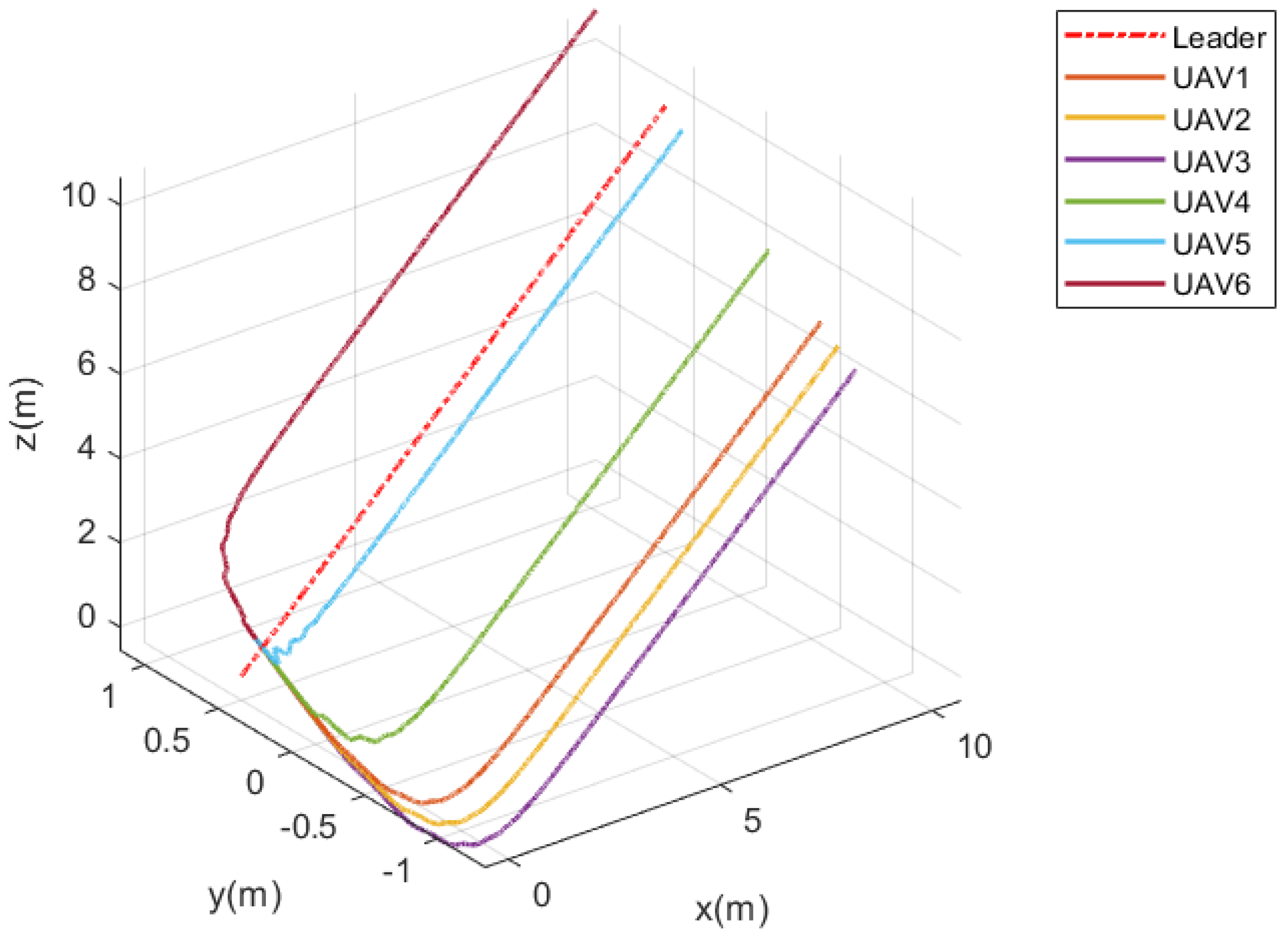
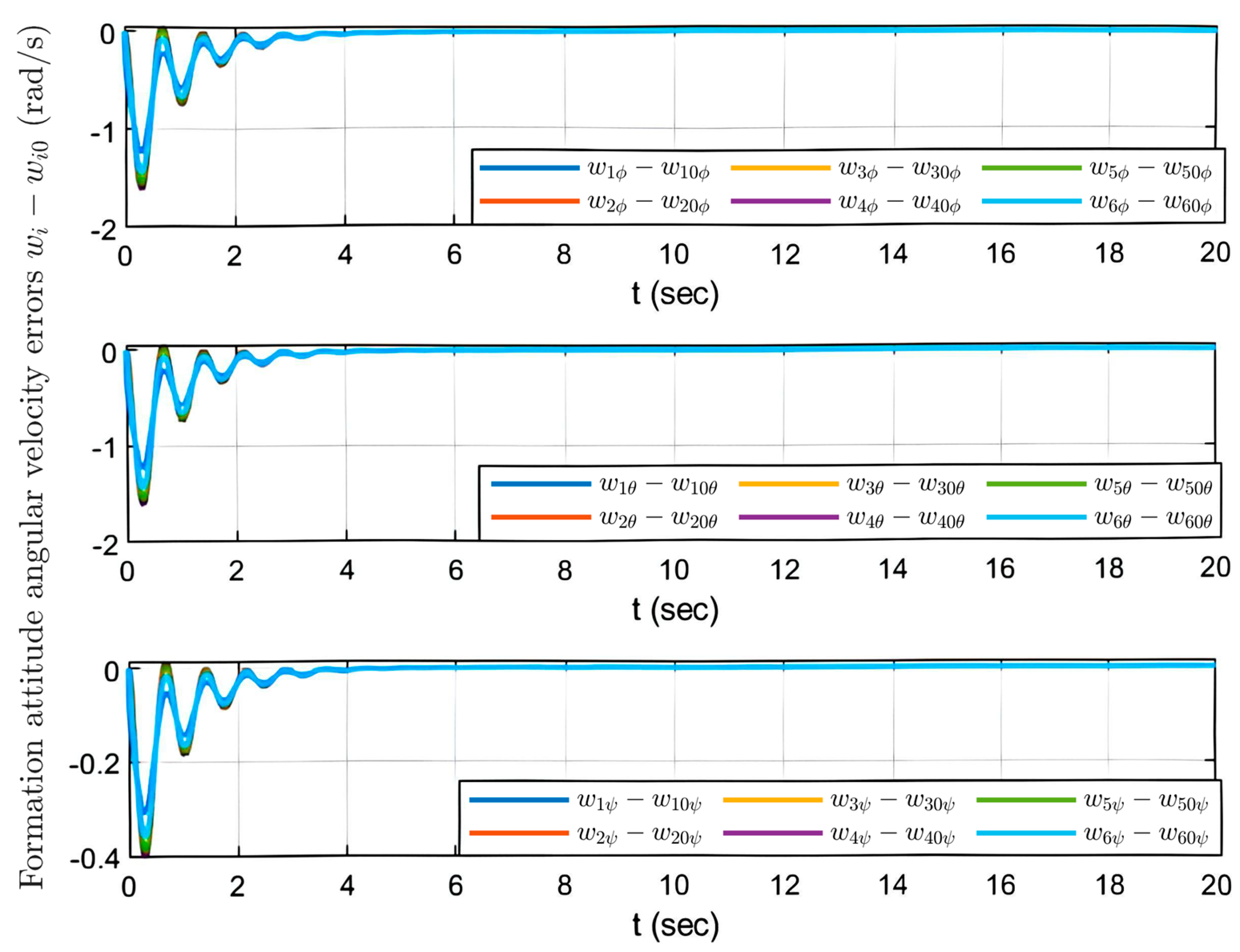
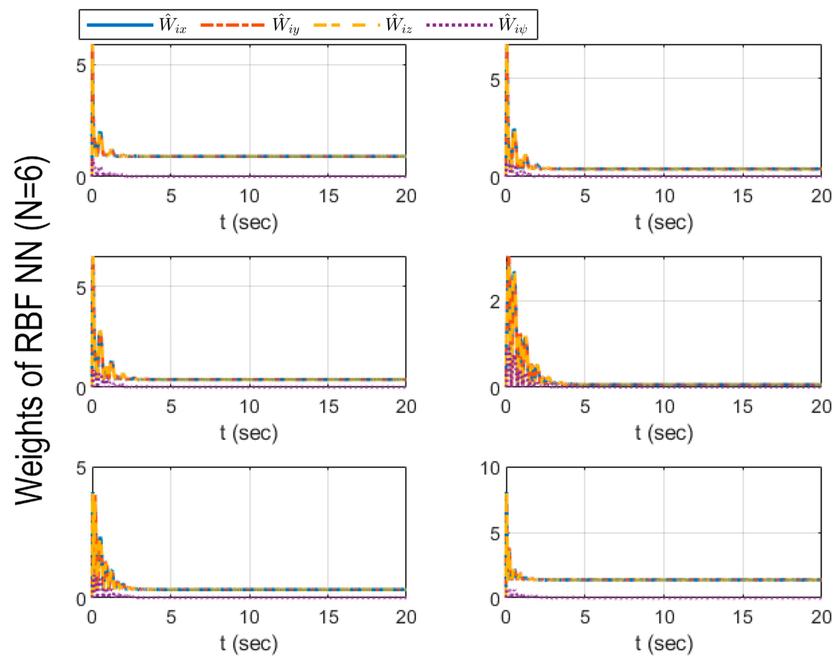
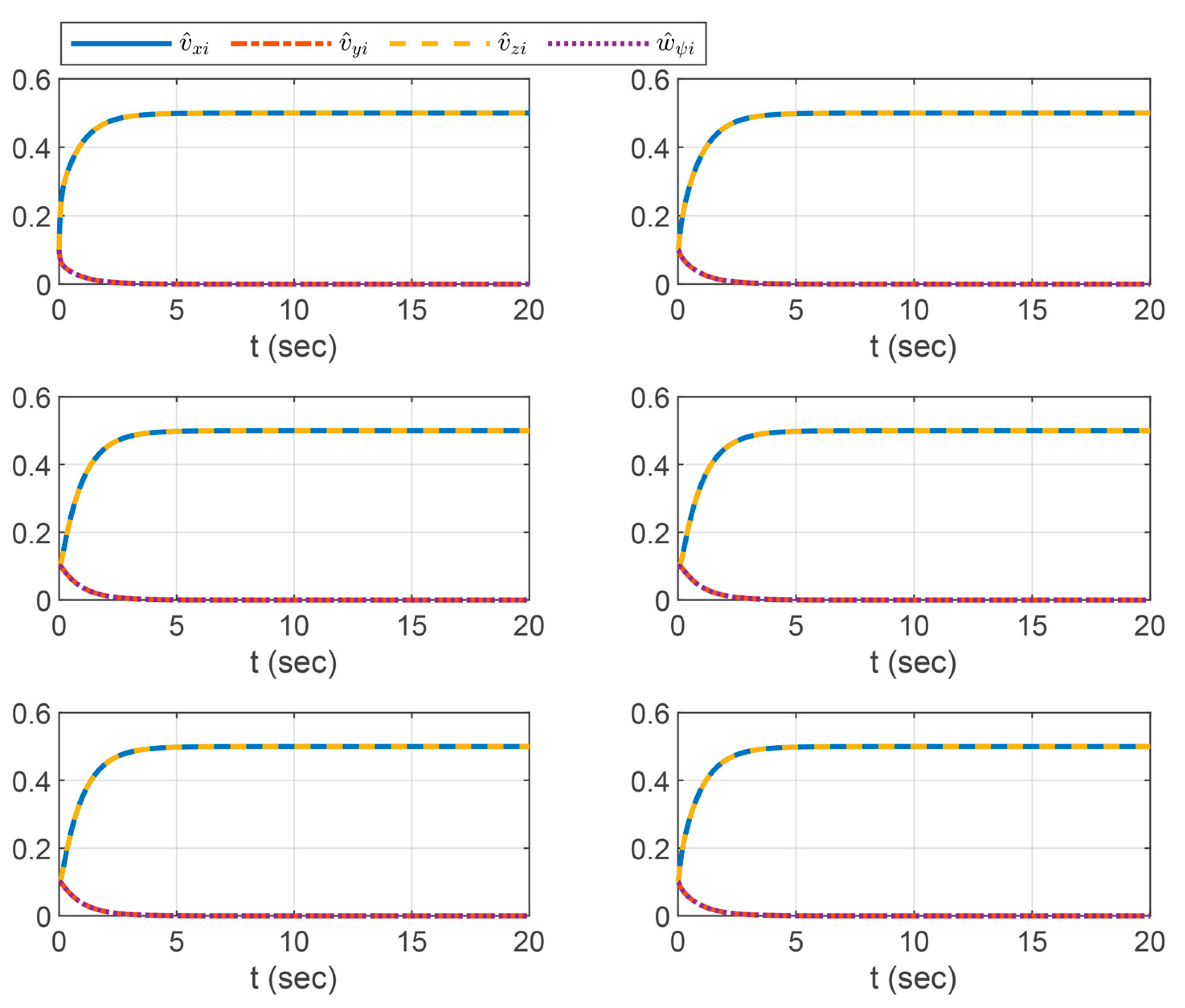
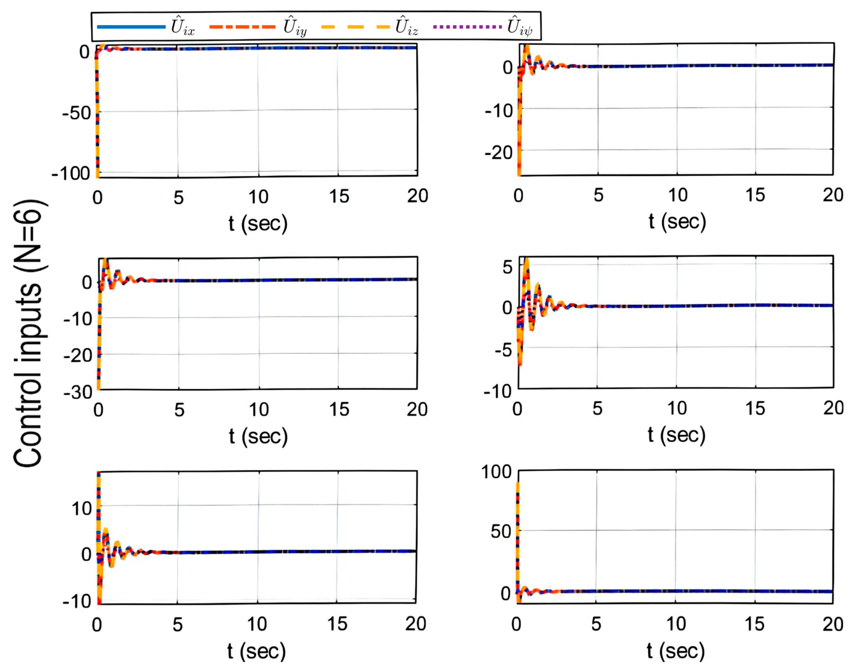
6. Numerical Simulations

This section presents MATLAB simulations involving six quadrotors ($n=6$) to validate the effectiveness and performance of the proposed control scheme. In this paper, MATLAB (SIMULINK) (MATLAB 2022b) is used as the Simulation Platform to evaluate the proposed neural network-based predefined-time controlled scheme, where the ode3 (fixed-step) Differentiation Method is utilized for the numerical integration of differential equations, with a Total Simulation Time of 20 s and a Sampling Time to 0.01 s.

The initial values are given by $q_i\left(0\right)={[x_i\left(0\right),y_i\left(0\right),z_i\left(0\right)]}^{\top }$, where $x_i\left(0\right),y_i\left(0\right),z_i\left(0\right)$ are randomly selected from the interval $(0,0.5]$. Additionally, the initial velocity is ${\dot{q}}_i\left(0\right)=v_i\left(0\right)={[0,0,0]}^{\top }$, the initial orientation is ${\psi }_i\left(0\right)={\left[{\displaystyle \frac{\pi }{3}},{\displaystyle \frac{\pi }{3}},{\displaystyle \frac{\pi }{3}}\right]}^{\top }$, and the initial angular velocity is ${\omega }_i\left(0\right)={[0,0,0]}^{\top }$. The external disturbances for each UAV are randomly given as ${\delta }_i={[0.5sin\left(t\right),0.5cos\left(t\right),0.5,0.5sin\left({\displaystyle \frac{\pi }{4}}t\right),0.5cos\left({\displaystyle \frac{\pi }{4}}t\right),0.25\pi t]}^{\top }$, and $i=1,2,\cdots ,6$.

The specific parameter values for the i-th quadrotor in the multi-UAV system, where $i=1,2,\dots ,6$, are as follows: The mass of the quadrotor is $m_i=2$ kg, the arm length is $l_i=0.2$ m, and the gravitational acceleration is $g=9.8$ m/s². The moments of inertia around the x-, y-, and z-axes are $I_{i1}=1.5$ N·s² ·rad⁻¹, $I_{i2}=1.5$ N·s²·rad⁻¹, and $I_{i3}=1.8$ N·s²·rad⁻¹, respectively. The drag coefficients for the system are $Q_{ix}=0.01$ N·s·rad⁻¹, $Q_{iy}=0.01$ N·s·rad⁻¹, and $Q_{iz}=0.01$ N·s·rad⁻¹, while the drag coefficients for the roll, pitch, and yaw angles are $Q_{i\varphi }=0.015$ N·s·rad⁻¹, $Q_{i\theta }=0.015$ N·s·rad⁻¹, and $Q_{i\psi }=0.015$ N·s·rad⁻¹, respectively.

Here, the model uncertainty is assumed to be one-tenth of the nominal model and randomly assigned to six quadrotors. The communication interaction network of the quadrotor fleet can be abstractly represented by Figure 4. The virtual leader is simulated as ${[0.5t,0.5,0.5t,\pi /4]}^{\top }$.

The convergence state of the formation tracking error of the controlled fleet is controlled by predefined-time constraints, which are $T_1+T_2=2$ and $T_1+T_2+T_3=4$. The parameters of the predefined-time control are set at ${\alpha }_1=0.5$, ${\alpha }_2=1.1$, ${\beta }_1=0.45$, ${\beta }_2=1.05$, ${\gamma }_1=0.45$, ${\gamma }_2=1.05$, ${\chi }_{q_1}=3.50$, ${\chi }_{q_2}=1.50$, ${\chi }_{q_3}=10.50$, and ${ϵ}_{{q_i}_{max}}=0.5$. The parameters of the corresponding attitude subsystem can refer to the position subsystem. The parameter selections for the RBF neural network are shown as ${\widehat{W}}_i\left(0\right)={\left[0\right]}_{12\times 2}$, $\mu$ is selected randomly, $b=10$, and $i=1,2,\cdots ,6$.

Next, we present the performance of the designed controller, with a simulation time lasting for 20 s.

Figure 5, Figure 6, Figure 7, Figure 8, Figure 9, Figure 10 and Figure 11 provide a comprehensive demonstration of the control performance of the proposed approach across five key aspects: the formation flight state of the three-dimensional trajectory, linear velocity tracking error, attitude tracking error, angular velocity tracking error, RBF neural network weights, desire velocity observation states, and control inputs. The results indicate that, with appropriate parameter selection, the formation tracking controller enables the quadrotor fleet to achieve predefined-time control within approximately 4 s while effectively overcoming the effects of model uncertainties and external disturbances.

7. Conclusions

This study has successfully developed a neural network-based predefined-time control strategy to address the distributed formation control problems for a team of quadrotor UAVs with model uncertainties and external disturbances. A distributed velocity observer is used to design the neural network-based predefined-time formation control strategy, where predefined-time control is first utilized to improve the robustness of the developed control strategy, and a neural network is then integrated to enhance its adaptability. Furthermore, the predefined-time stability of the closed-loop control system is rigorously validated using Lyapunov stability analysis, and MATLAB-based simulations are provided to verify the developed neural network-based predefined-time scheme, as well as its overall cooperative performance involving stability, adaptability, and robustness.

In future work, we will primarily focus on the distributed coordinated formation control problems for swarm quadrotor UAVs from the perspective of both the intelligent era and space or aerial engineering missions, considering important technical issues such as appointed-time control, input saturation control, and fault diagnosis and fault-tolerant control, as well as implementing real experimental investigations for multi-quadrotor UAVs.

References

1. Liu, K.; Wang, R.J.; Wang, X.D.; Wang, X.X. Anti-Saturation Adaptive Finite-Time Neural Network-Based Fault-Tolerant Tracking Control for a Quadrotor UAV with External Disturbances. Aerosp. Sci. Technol. 2021, 115, 106790. [Google Scholar] [CrossRef]
2. Erdelj, M.; Natalizio, E.; Chowdhury, K.R.; Akyildiz, I.F. Help from the Sky: Leveraging UAVs for Disaster Management. IEEE Pervasive Comput. 2017, 16, 24–32. [Google Scholar] [CrossRef]
3. Ramirez-Rodriguez, H.; Parra-Vega, V.; Sanchez-Orta, A.; Garcia-Salazar, O. Robust Backstepping Control Based on Integral Sliding Modes for Tracking of Quadrotors. J. Intell. Robot. Syst. 2014, 73, 51–66. [Google Scholar] [CrossRef]
4. Wang, B.; Li, Q.; Mao, Q.; Wang, J.; Chen, C.L.P.; Shangguan, A.; Zhang, H. A Survey on Vision-Based Anti Unmanned Aerial Vehicles Methods. Drones 2024, 8, 518. [Google Scholar] [CrossRef]
5. Nettari, Y.; Labbadi, M.; Kurt, S. Adaptive Robust Finite-Time Tracking Control for Quadrotor Subject to Disturbances. Adv. Space Res. 2023, 71, 3803–3821. [Google Scholar] [CrossRef]
6. Zhu, P.F.; Wen, L.Y.; Du, D.W.; Bian, X.; Fan, H.; Hu, Q.H.; Ling, H.B. Detection and Tracking Meet Drones Challenge. IEEE Trans. Pattern Anal. Mach. Intell. 2022, 44, 7380–7399. [Google Scholar] [CrossRef]
7. Idrissi, M.; Salami, M.; Annaz, F. A Review of Quadrotor Unmanned Aerial Vehicles: Applications, Architectural Design and Control Algorithms. J. Intell. Robot. Syst. 2022, 104, 22. [Google Scholar] [CrossRef]
8. Pan, J.S.; Lv, J.X.; Yan, L.J.; Weng, S.W.; Chu, S.C.; Xue, J.K. Golden Eagle Optimizer with Double Learning Strategies for 3D Path Planning of UAV in Power Inspection. Math. Comput. Simul. 2022, 193, 509–532. [Google Scholar] [CrossRef]
9. Wei, L.; Chen, M. Distributed DETMs-Based Internal Collision Avoidance Control for UAV Formation with Lumped Disturbances. Appl. Math. Comput. 2022, 433, 127362. [Google Scholar] [CrossRef]
10. Huang, F.J.; Wu, P.L.; Li, X.X. Distributed Flocking Control of Quad-rotor UAVs with Obstacle Avoidance Under the Parallel-triggered Scheme. Int. J. Control Autom. Syst. 2021, 19, 1375–1383. [Google Scholar] [CrossRef]
11. Fu, X.; Peng, J. Iterative Learning Control for UAVs Formation Based on Point-to-Point Trajectory Update Tracking. Math. Comput. Simul. 2023, 209, 1–15. [Google Scholar] [CrossRef]
12. Wang, H.P.; Song, S.Y.; Guo, Q.H.; Xu, D.; Zhang, X.Y.; Wang, P.Z. Cooperative Motion Planning for Persistent 3D Visual Coverage with Multiple Quadrotor UAVs. IEEE Trans. Autom. Sci. Eng. 2024, 21, 3374–3383. [Google Scholar] [CrossRef]
13. Mofid, O.; Mobayen, S.; Zhang, C.; Esakki, B. Desired Tracking of Delayed Quadrotor UAV Under Model Uncertainty and Wind Disturbance Using Adaptive Super-Twisting Terminal Sliding Mode Control. ISA Trans. 2022, 123, 455–471. [Google Scholar] [CrossRef]
14. Li, J.; Zhao, Z.; Qin, X. Adaptive Sliding Mode Control Using a Novel Fully Feedback Recurrent Neural Network for Quadrotor UAVs. Neurocomputing 2024, 610, 128592. [Google Scholar] [CrossRef]
15. Mofid, O.; Mobayen, S. Adaptive Finite-Time Backstepping Global Sliding Mode Tracker of Quad-Rotor UAVs Under Model Uncertainty, Wind Perturbation, and Input Saturation. IEEE Trans. Aerosp. Electron. Syst. 2022, 58, 140–151. [Google Scholar] [CrossRef]
16. Aspragkathos, S.N.; Karras, G.C.; Kyriakopoulos, K.J. Event-Triggered Image Moments Predictive Control for Tracking Evolving Features Using UAVs. IEEE Robot. Autom. Lett. 2024, 9, 1019–1026. [Google Scholar] [CrossRef]
17. Liu, K.; Yang, P.; Wang, R.J.; Jiao, L.; Li, T.; Zhang, J. Observer-Based Adaptive Fuzzy Finite-Time Attitude Control for Quadrotor UAVs. IEEE Trans. Aerosp. Electron. Syst. 2023, 59, 8637–8654. [Google Scholar] [CrossRef]
18. Liu, K.; Yang, P.; Jiao, L.; Wang, R.J.; Yuan, Z.P.; Dong, S.F. Antisaturation Fixed-Time Attitude Tracking Control Based on Low-Computation Learning for Uncertain Quadrotor UAVs with External Disturbances. Aerosp. Sci. Technol. 2023, 142, 108668. [Google Scholar] [CrossRef]
19. Wen, S.Q.; Tong, S.C. Observer-Based Adaptive Neural Network Inverse Optimal Containment Control for Nonlinear Multiagent Systems with Input Quantization. Neurocomputing 2024, 592, 127796. [Google Scholar] [CrossRef]
20. Gong, B.; Li, Y.; Zhang, L.; Ai, J. Adaptive Factor Fuzzy Controller for Keeping Multi-UAV Formation While Avoiding Dynamic Obstacles. Drones 2024, 8, 344. [Google Scholar] [CrossRef]
21. Du, Z.; Zhang, H.; Wang, Z.; Yan, H. Model Predictive Formation Tracking-Containment Control for Multi-UAVs with Obstacle Avoidance. IEEE Trans. Syst. Man-Cybern.-Syst. 2024, 54, 3404–3414. [Google Scholar] [CrossRef]
22. Xia, K.; Li, X.; Li, K.; Zou, Y. Distributed Predefined-Time Control for Cooperative Tracking of Multiple Quadrotor UAVs. IEEE/CAA J. Autom. Sin. 2024, 11, 2179–2181. [Google Scholar] [CrossRef]
23. Wang, H.; Li, M.; Zhang, H.; Liu, S. Predefined-Time Composite Adaptive Fuzzy Nonsingular Attitude Control for Multi-UAVs. IEEE Trans. Fuzzy Syst. 2024. [Google Scholar] [CrossRef]
24. Guo, K.; Li, X.; Xie, L. Ultra-Wideband and Odometry-Based Cooperative Relative Localization with Application to Multi-UAV Formation Control. IEEE Trans. Cybern. 2020, 50, 2590–2603. [Google Scholar] [CrossRef]
25. Madhiarasan, M.; Louzazni, M. Analysis of Artificial Neural Network: Architecture, Types, and Forecasting Applications. J. Electr. Comput. Eng. 2022, 2022, 5416722. [Google Scholar] [CrossRef]
26. Zhao, A.; Toudeshki, A.; Ehsani, R.; Sun, J.Q. Data-Driven Inverse Kinematics Approximation of a Delta Robot with Stepper Motors. Robotics 2023, 12, 135. [Google Scholar] [CrossRef]
27. Guo, W.; Shi, L.; Sun, W.; Jahanshahi, H. Predefined-Time Average Consensus Control for Heterogeneous Nonlinear Multi-Agent Systems. IEEE Trans. Circuits Syst. II Express Briefs 2023, 70, 2989–2993. [Google Scholar] [CrossRef]
28. Wang, J.; Fang, X.; Li, X. Predefined-Time Platoon Control of Unmanned Aerial Vehicle with Range-Limited Communication. Drones 2024, 8, 263. [Google Scholar] [CrossRef]
29. Ding, J.; Jiang, X.; Zou, Y.; Tang, Z.; Zhen, Z. A Multivariable Adaptive Formation Control for Multiple UAVs with External Uncertain Disturbances. Aircr. Eng. Aerosp. Technol. 2025, 97, 170–178. [Google Scholar] [CrossRef]
30. Liu, Y.; Chen, C.; Wang, Y.; Zhang, T.; Gong, Y. A Fast Formation Obstacle Avoidance Algorithm for Clustered UAVs Based on Artificial Potential Field. Aerosp. Sci. Technol. 2024, 147, 108974. [Google Scholar] [CrossRef]
31. Li, N.; Wang, H.; Luo, Q.; Zheng, W. Distributed Formation Control for Multiple Quadrotor UAVs Based on Distributed Estimator and Singular Perturbation System. Int. J. Control Autom. Syst. 2024, 22, 1349–1359. [Google Scholar] [CrossRef]
32. Hartley, J.; Shum, H.P.; Ho, E.S.; Wang, H.; Ramamoorthy, S. Formation Control for UAVs Using a Flux-Guided Approach. Expert Syst. Appl. 2022, 205, 117665. [Google Scholar] [CrossRef]
33. Li, Y.; Li, H.; Ding, X.; Zhao, G. Leader-Follower Consensus of Multiagent Systems with Time Delays Over Finite Fields. IEEE Trans. Cybern. 2019, 49, 3203–3208. [Google Scholar] [CrossRef] [PubMed]
34. Aldana-López, R.; Gómez-Gutiérrez, D.; Jiménez-Rodríguez, E.; Sánchez-Torres, J.D.; Defoort, M. Enhancing the Settling Time Estimation of a Class of Fixed-Time Stable Systems. Int. J. Robust Nonlinear Control 2019, 29, 4135–4148. [Google Scholar] [CrossRef]
35. Chen, B.; Zhang, H.; Lin, C. Observer-Based Adaptive Neural Network Control for Nonlinear Systems in Nonstrict-Feedback Form. IEEE Trans. Neural Netw. Learn. Syst. 2016, 27, 89–98. [Google Scholar] [CrossRef]
36. Xiong, J.J.; Zhang, G.B. Global Fast Dynamic Terminal Sliding Mode Control for a Quadrotor UAV. ISA Trans. 2017, 66, 233–240. [Google Scholar] [CrossRef]
37. Okasha, M.; Kralev, J.; Islam, M. Design and Experimental Comparison of PID, LQR and MPC Stabilizing Controllers for Parrot Mambo Mini-Drone. Aerospace 2022, 9, 298. [Google Scholar] [CrossRef]
38. Yu, Y.; Guo, J.; Ahn, C.K.; Xiang, Z. Neural Adaptive Distributed Formation Control of Nonlinear Multi-UAVs with Unmodeled Dynamics. IEEE Trans. Neural Netw. Learn. Syst. 2022, 34, 9555–9561. [Google Scholar] [CrossRef]
39. Gao, H.; Xia, Y.; Liu, K.; Zhang, J.; Cui, B. Resilient Neuroadaptive Distributed Fixed-Time Attitude Coordination Control for Multiple Spacecraft. IEEE Trans. Cybern. 2024, 54, 4973–4985. [Google Scholar] [CrossRef]
40. Dong, X.; Zhou, Y.; Ren, Z.; Zhong, Y. Time-Varying Formation Tracking for Second-Order Multi-Agent Systems Subjected to Switching Topologies with Application to Quadrotor Formation Flying. IEEE Trans. Ind. Electron. 2017, 64, 5014–5024. [Google Scholar] [CrossRef]
Figure 1. The RBF neural network structure.
Drones 09 00222 g001
Figure 2. The quadrotor UAV model diagram.
Drones 09 00222 g002
Figure 3. The control structure of the quadrotor UAVs.
Drones 09 00222 g003
Figure 4. Communication topologies with six UAVs.
Drones 09 00222 g004
Figure 5. Trajectory status chart with proposed controller.
Drones 09 00222 g005
Figure 6. Velocity tracking errors with proposed controller, where v 0 represents the leader’s velocity.
Drones 09 00222 g006
Figure 7. Attitude tracking errors with proposed controller.
Drones 09 00222 g007
Figure 8. Angular velocity tracking errors with proposed controller, where ω i 0 represents the leader’s angular velocity.
Drones 09 00222 g008
Figure 9. Weights of RBF neural network.
Drones 09 00222 g009
Figure 10. Desired velocity observation states ( v ^ x i ( 0 ) = v ^ y i ( 0 ) = v ^ z i ( 0 ) = ω ^ ψ i ( 0 ) = 0.1 ) .
Drones 09 00222 g010
Figure 11. Control inputs.
Drones 09 00222 g011
Disclaimer/Publisher’s Note: The statements, opinions and data contained in all publications are solely those of the individual author(s) and contributor(s) and not of MDPI and/or the editor(s). MDPI and/or the editor(s) disclaim responsibility for any injury to people or property resulting from any ideas, methods, instructions or products referred to in the content.