Article

Exploring the Feasibility of Airfoil Integration on a Multirotor Frame for Enhanced Aerodynamic Performance

by
António André C. Freitas
1,*,
Victor Wilson G. Azevedo
1,
Vitor Hugo A. Aguiar
1,
Jorge Miguel A. Lopes
1 and
Rui Miguel A. Caldeira
1,2
1
ARDITI—Agência Regional para o Desenvolvimento da Investigação, Tecnologia e Inovação, Edif. Madeira Tecnopolo, Piso 2, Caminho da Penteada, 9020-105 Funchal, Portugal
2
OOM—Observatório Oceânico da Madeira, Edifício Madeira Tecnopolo, Piso 0, Caminho da Penteada, 9020-105 Funchal, Portugal
*
Author to whom correspondence should be addressed.
Drones 2025, 9(3), 202; https://doi.org/10.3390/drones9030202
Submission received: 21 February 2025 / Revised: 5 March 2025 / Accepted: 7 March 2025 / Published: 12 March 2025

Abstract

:
Unmanned Aerial Vehicles (UAVs) have become indispensable across various industries, but their efficiency, particularly in multirotor designs, remains constrained by aerodynamic limitations. This study investigates the integration of airfoil shapes into the arms of multirotor UAV frames to enhance aerodynamic performance, thereby improving energy efficiency and extending flight times. By employing Computational Fluid Dynamics (CFD) simulations, this research compares the aerodynamic characteristics of a standard quadrotor frame against an airfoil-integrated design. The results reveal that while airfoil-shaped arms marginally increase drag in cruise flight, they significantly reduce downforce across all flight conditions, optimizing thrust utilization and lowering overall energy consumption. The findings suggest potential applications in military reconnaissance, agriculture, and other fields requiring longer UAV flight durations and improved efficiency. This work advances UAV design by demonstrating a feasible method for enhancing the performance of multirotor systems while maintaining structural simplicity and cost-effectiveness.

1. Introduction

The term Unmanned Air Vehicle (UAV) refers to any aircraft that can fly without a person onboard to control it. This term is commonly used in the computer science and artificial intelligence community. However, other terms such as Remotely Piloted Vehicle (RPV) [1], Remotely Operated Aircraft (ROA) [2], Unmanned Vehicle Systems (UVSs) [3], and, more commonly, drones [4] are also used.
At present, UAVs are a crucial piece of technology for various industries due to their versatility, accessibility, and advanced technological capabilities. Nahiyoon et al. [5] mentioned how the use of UAVs for plant protection plays a vital role in modern agricultural operations. Frachtenberg [6] described the UAV’s capacity to transform the delivery services industry and, consequently, society as a whole. Viana et al. [7] believe that UAVs’ relays can play a critical role in 5G public safety communications. Álvarez González et al. [8] affirm that UAVs can be a valuable, non-invasive, and useful tool for a wide range of applications in marine mammal research. Munawar et al. [9] state that the inspection of infrastructure damages such as building cracks can be automated using UAVs for aerial imagery of damages and explore different approaches based on artificial intelligence (AI) and machine learning (ML) techniques. Pan et al. [10] address the use of UAVs for military scenarios and the generation of vast amounts of image data that can be leveraged for textual intelligence generation to support military decision-making. These are only some examples of industries where UAVs have acquired a critical role.
This article addresses the design of UAVs for military defense, aiming to enhance their aerodynamic efficiency and extend their flight duration. The findings from this study are also relevant to other industries.

1.1. Motivation

The entity funding this research and development project showed interest in the development of a small-sized UAV with the main focus of performing medium- to long-range cruise flights at low altitude and high speed, as well as close-range inspections and reconnaissance missions.
There are several types of UAVs, each with unique features and capabilities tailored to specific applications and environments. In terms of their structure, according to Rennie [11], there are three main types:
  • Fixed-wing UAVs have a design similar to traditional airplanes featuring a rigid wing structure. Lift is generated by horizontal airflow flowing over the main wing, while horizontal thrust is provided by motors. The aircraft is navigated using control surfaces such as ailerons, elevators, and rudders;
  • Rotary-wing UAVs can be categorized as either multirotor or single-rotor. These rely on rotors for both lift and control, which enables them to hover in one place and perform vertical takeoff and landing (VTOL) unlike the fixed-wing UAVs. However, this advantage comes with a trade-off: rotary-wing UAVs typically have shorter flight times. Among these, multirotors are the most common type;
  • Hybrids, as the name suggests, combine features of fixed-wing and rotary-wing UAVs, commonly using the fixed-wing configuration for cruise flight and rotary-wing configuration for takeoff, hover, and landing.
Considering the different types of UAVs previously discussed, one might conclude that a Hybrid UAV is the most suitable option for this mission since fixed wings cannot hover and rotary wings are not efficient for long cruise flights. However, common Hybrid UAVs come with specific disadvantages that could impact their effectiveness for this mission. For instance, as noted by Ducard et al. [12], they require a significant wingspan to achieve efficient cruising and show reduced agility, wind resistance, and hovering efficiency compared to multirotors.
Examining the research performed by Kunertova [13] and Seo et al. [14] on the ongoing conflicts in Eastern Europe provides valuable insights into the types of drones commonly used in military interventions and defense operations. It is evident that small-sized UAVs, particularly simple “do it yourself (DIY)” carbon fiber quadrotors, have significantly impacted the nature of close-range warfare due to their numerous advantages. This raises an important question: is it possible to enhance the efficiency of these UAVs, enabling them to take part in medium- to long-range missions?

1.2. Objective

Taking into account what was previously said, the primary aim of this study is to enhance the aerodynamic efficiency of a simple carbon frame UAV. This vehicle should be easy to deploy, lightweight for easy transportation, cost-effective, low-maintenance, capable of efficiently flying long distances, and able to successfully conduct close-range reconnaissance missions.
Thus, this study explores the feasibility of developing a unique Hybrid UAV that combines a traditional quadrotor frame with a fixed wing. Unlike standard fixed-wing UAVs, where the fixed wing generates all the lift during cruise flight, this research hypothesizes that the arms of the multirotor—typically used solely to support the motors—can be designed as airfoils. If, in order to clarify the work performed, the aerodynamic drag force acting on the UAV is decomposed into a vertical component called downforce and a horizontal component simply referred to as drag, then this design aims to reduce both, thereby decreasing the load on the motors, which in turn lowers energy consumption and increases flight time. To investigate this concept, Computational Fluid Dynamics (CFD) analyses were conducted, comparing the newly developed “airfoil frame” with conventional quadrotor First-Person View (FPV) frames, referred to hereafter as the “standard frame”.

1.3. Research Contributions

The integration of airfoil structures into multirotor UAV frames represents an emerging area of research aimed at improving aerodynamic efficiency and extending flight performance. While traditional multirotor designs prioritize maneuverability and stability, they often suffer from high energy consumption due to inherent aerodynamic inefficiencies, particularly the generation of downforce and excessive drag. To address the existing limitations in UAV efficiency, this research makes the following key contributions:
  • A novel investigation into the integration of airfoil-shaped arms in a multirotor UAV to enhance aerodynamic efficiency;
  • CFD analysis comparing a standard quadrotor frame with an airfoil-integrated design, assessing aerodynamic benefits;
  • A detailed evaluation of the impact of airfoil integration on downforce, drag, and flight time across different flight conditions;
  • A methodology for designing and implementing airfoil structures in multirotor UAV frames without increasing structural complexity;
  • Insights into the potential applications of airfoil-integrated UAVs in military, agricultural, and industrial settings, emphasizing efficiency improvements.
By providing a detailed assessment of airfoil integration in multirotor UAVs, this research advances the field of UAV design and lays the groundwork for future experimental validation and real-world applications.

2. Multirotor UAV Development Considerations

This section aims to provide a clear overview of the main steps involved in the development process of multirotor UAVs. It begins with selecting the frame and components suited for specific missions and then discusses proposed modifications to enhance the aerodynamic efficiency of the multirotor. The recommended manufacturing process for the modified parts is addressed in Appendix C. Additionally, this section outlines the scientific method used to theoretically confirm whether these modifications lead to increased efficiency.

2.1. UAV Component Selection

The success of a military UAV survey mission relies on the vehicle’s flight performance and efficiency, which are directly linked to the selection of its components, as noted by Stewart et al. [15].
As noted by Liu et al. [16], flight performance can be assessed based on several key factors: thrust, power, endurance, stability, and control. The selection of the motor and propeller is critical for the UAV’s ability to generate adequate thrust. If the motor is underpowered, the UAV may struggle to achieve the necessary altitude, speed, or maneuverability. Additionally, there is a strong relationship between battery capacity, its chemistry, and the propulsion system, all of which directly affect the UAV’s flight time, as demonstrated by Biczyski et al. [17]. Finally, Stewart et al. [15] note that to ensure stable flight and precise control, the flight controller, sensors (such as gyroscopes, accelerometers, and GPS), and optional actuators (such as servos) must be well matched.
Nagel [18] showed an example that efficiency is influenced not only by the propulsion system but also by the overall weight of the aircraft. Heavier UAVs require more power to remain airborne, which results in reduced flight times. To enhance efficiency, it is essential to choose lightweight components and payloads that ensure a balance between performance and weight. Additionally, Kumar et al. [19] state the importance of selecting appropriate materials for the aircraft’s frame, as these materials must achieve a balance between strength and weight.
It is also important to consider the specific mission requirements for the UAV. The selection of the power source, propulsion system, and frame components must align with the weight and power needs of the particular payloads, such as cameras, sensors, or delivery packages, while ensuring optimal flight performance is maintained. Additionally, communication systems, antennas, and navigation systems should be compatible with the UAV’s operational range and altitude capabilities. All chosen components must be durable enough to withstand various environmental conditions, including high altitudes, extreme temperatures, and windy conditions, without compromising performance.
Even though this study is theoretical and the described multirotor will not be constructed or flown, it is the basis for an operational model, so a brief explanation for the reasoning behind the selection of each propulsion-related component is provided in Appendix A. This is crucial as it allows for estimating the flight performance of the multirotor under study and analyzing the resulting data.

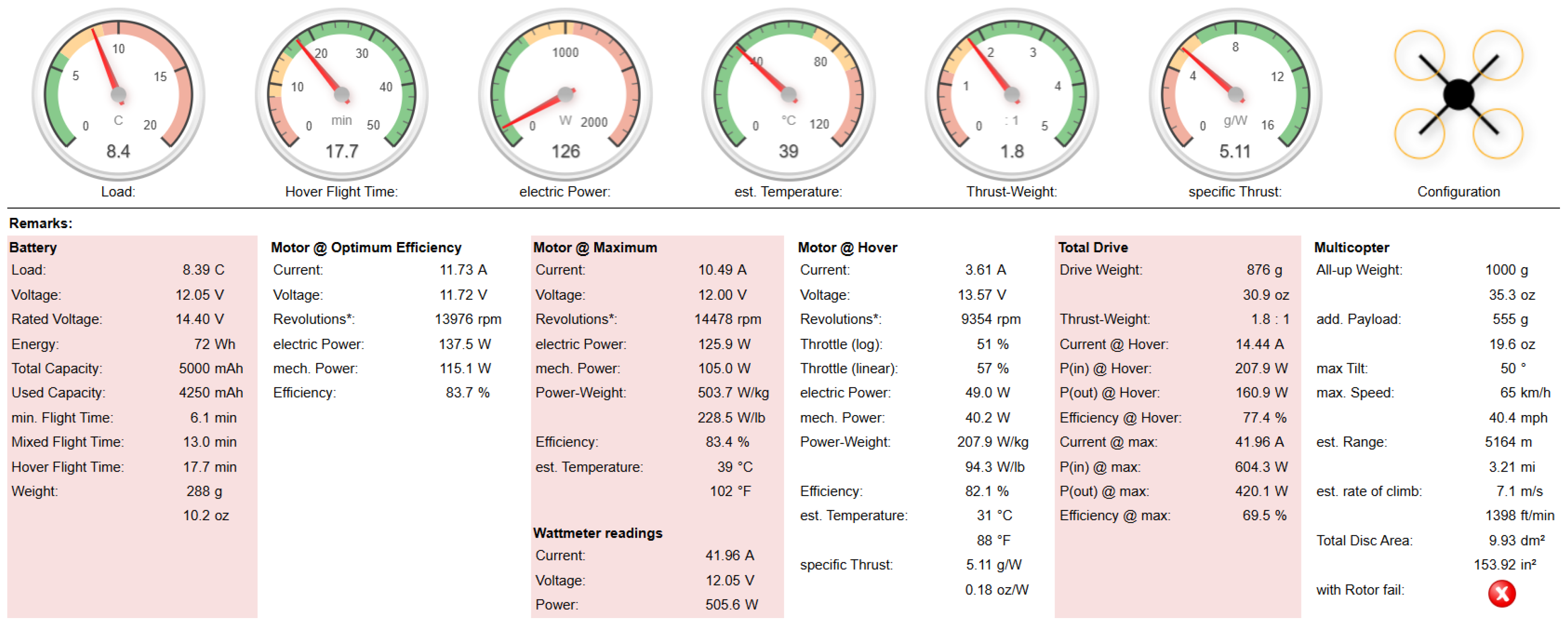
2.2. eCalc Simulator

Müller developed a popular online tool used by UAV developers, designated as eCalc [20], that helps to design and optimize vehicles by providing detailed calculations related to the power system and flight performance.
After completing the UAV component selection process, described in Section 2.1, the user can input the selected components into this tool to obtain a relatively accurate estimate of flight time, thrust-to-weight ratio, hover throttle, and overall efficiency, with a margin of error of ±15%. Following this, the user can analyze and optimize the UAV’s performance characteristics by adjusting the components based on the results. The goal is to find the best balance between power, weight, efficiency, and flight time. This process involves iterating multiple simulations and fine-tuning the component configurations until the performance objectives are met.
eCalc helps predict how a UAV will perform even before the building process begins. It ensures that all propulsion components are well matched, which helps prevent common issues such as overheating or underperformance. Additionally, a significant benefit of using eCalc is the potential savings in both time and money by avoiding incorrect component selection.

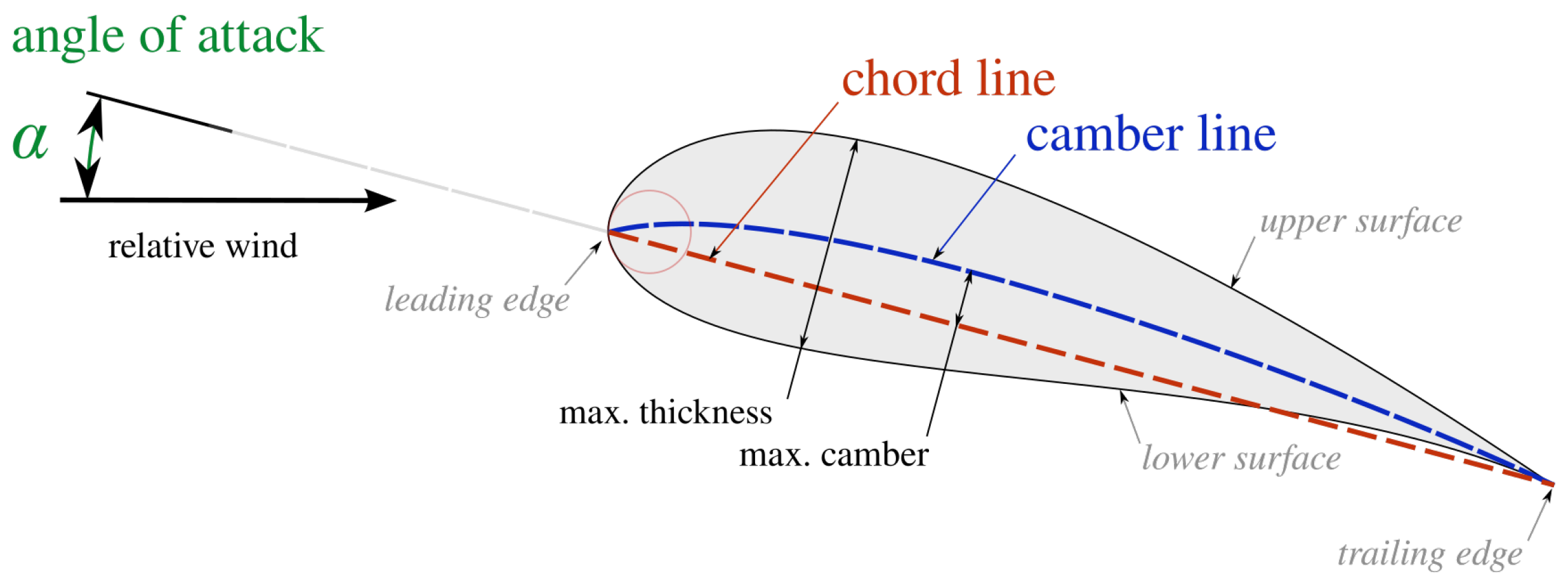
2.3. Airfoil Design and Selection

As previously noted, the aim of this analysis is to explore the potential for improving efficiency by adapting airfoils within a standard multirotor frame. Therefore, it is important to examine methods for airfoil design (Figure 1) and selection, as demonstrated by Eppler [21].
According to AirShaper [23], the key parameters that define an airfoil are as follows:
  • Leading edge—at the front of the airfoil;
  • Trailing edge—at the rear of the airfoil;
  • Chord line—defined by drawing a straight line from the leading edge to the trailing edge;
  • Camber line—represents the center line between the upper and lower surfaces;
  • Angle of attack (AoA)—the angle between the chord line and the relative wind direction.
The airflow direction relative to an airfoil can be determined by analyzing the velocity vectors of both the wind and the airfoil.
The total force generated by an airfoil is typically divided into two components: lift ( F L ) and drag ( F D ). The drag force is measured along the direction of the airflow, while the lift force is measured perpendicular to that direction.
To compare the performance of different airfoils, two key parameters are used: the lift coefficient ( C L ) and the drag coefficient ( C D ). These coefficients normalize the lift and drag forces based on the wing area and dynamic pressure, which is related to the flow speed. This approach allows for a consistent comparison of airfoil performance, regardless of variations in wing sizes and flow speeds.
According to Anderson [24], the drag and lift coefficients are computed using the following formulas:
C D = 2 F D ρ v 2 A
C L = 2 F L ρ v 2 A
where the following are true:
  • F D = drag force [N];
  • F L = lift force [N];
  • ρ = density of the fluid [kg/m3];
  • v = fluid velocity relative to the body [m/s];
  • A = reference cross-sectional area [m2].
The behavior of an airfoil is influenced by the Reynolds number (Re), a dimensionless parameter that represents the ratio of inertial forces to viscous forces in a fluid flow, as outlined by LaNasa et al. [25]. The Reynolds number depends on fluid density, velocity, viscosity, and the chord length of the airfoil. It plays a crucial role in determining whether the flow around the airfoil is laminar or turbulent, which in turn affects drag, lift, and other aerodynamic characteristics.
The lift and drag forces generated by an airfoil vary with the flow’s AoA. The lift coefficient and, consequently, the lift force increase with the AoA until it reaches a critical point known as the stall point, as illustrated in Figure 2. This occurs due to boundary layer separation on the upper surface of the airfoil. Similarly, the drag coefficient and drag force also rise with increasing AoA.
Haryanto et al. [26] demonstrated that the lift-to-drag ratio ( C L C D ) is frequently used to evaluate airfoil performance. A higher ratio signifies a more efficient design.
Figure 2. The coefficient of lift ( C L ) and coefficient of drag ( C D ) and their ratio as a function of the angle of attack for a hypothetical wing. Additionally, the flow status from attached to separated is shown in relation to the curve [27].
Drones 09 00202 g002
Additionally, there are two types of airfoils: symmetric and asymmetric, each offering different performance characteristics, as noted by Kay et al. [28]. Asymmetric airfoils feature a curved camber line, and when chosen appropriately, they can generate higher lift values with greater efficiency. However, this comes at the cost of reduced performance at negative angles of attack, resulting in a narrower effective operating range.

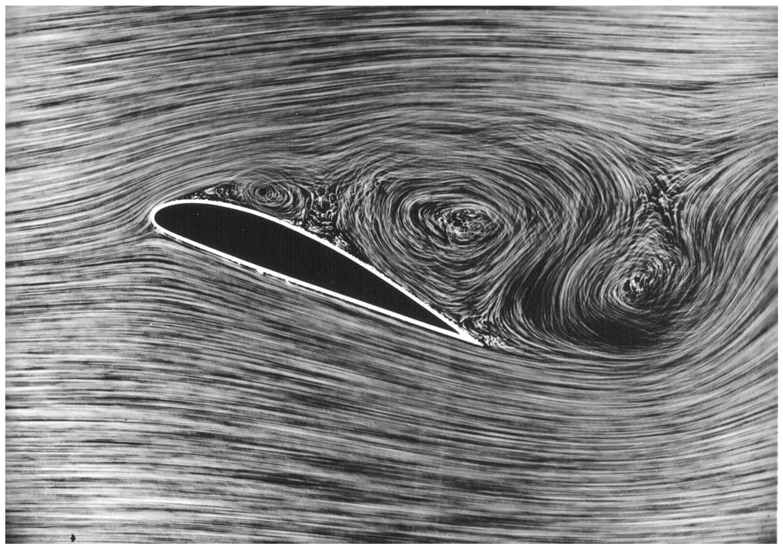
2.3.1. Flow Visualization and Separation

When an object moves through a fluid, understanding the interactions between the two can be challenging. Flow visualization, as noted by Merzkirch [29], is a useful and cost-effective method for gaining insight into qualitative flow patterns and fluid properties around an object (see Figure 3). This technique helps distinguish areas of clean airflow from regions of turbulence and flow separation. While flow visualization does not replace actual data, it can offer valuable insights into the performance of aerodynamic devices and the reasons behind their effectiveness.
According to Chang [30], flow separation occurs when the air flowing around an object can no longer adhere to its contour and physically disengages from the surface. This phenomenon is primarily caused by sharp edges in the object’s geometry or an adverse pressure gradient.
Fluid naturally flows from areas of high pressure to low pressure, which is referred to as a favorable pressure gradient. Conversely, an adverse pressure gradient occurs when static pressure increases in the direction of the flow. In this case, air is compelled to move from a low-pressure zone to a high-pressure zone, which requires energy and results in a slowdown of the flow.
When this slowdown happens near the surface of an object, the flow decelerates to the point where it changes direction. This point is known as the separation point, beyond which the flow can no longer follow the surface profile.
Figure 3. Visualization of flow separation behind an airfoil, provided by Prandtl [31].
Drones 09 00202 g003

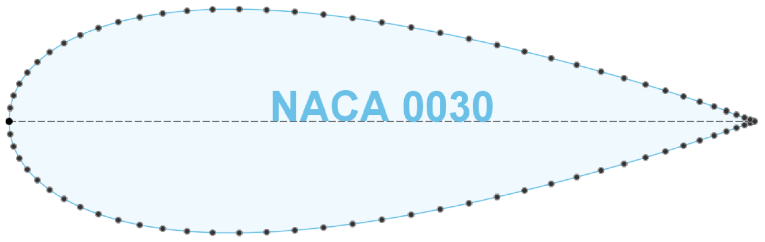
2.3.2. NACA Airfoils

According to Abbott et al. [32], the National Advisory Committee for Aeronautics (NACA) developed a series of airfoils during the 1920s. These airfoils were thoroughly tested and assigned a numerical designation that represented their critical geometric properties, including camber lines, maximum thickness, and special nose features. This systematic approach resulted in families of airfoils with specific aerodynamic characteristics, enabling engineers to select the appropriate airfoil for the desired performance of each aircraft.
The key reasons for selecting a NACA airfoil instead of creating a custom design include the extensive performance data already available, the efficiency of their design, ease of manufacturing, versatility, and their status as industry standards. The compatibility with existing tools and benchmarks further enhances their appeal.
Appendix B briefly addresses the NACA airfoil families and explores the advantages, disadvantages, and applications of each one.

2.4. Computational Fluid Dynamics

Anderson et al. [33] indicate that CFD origins are deeply tied to advances in both theoretical fluid dynamics and computational technology.
It began to take shape in the 1940s and 1950s with attempts to solve complex flow problems that could not be addressed by traditional experimental or theoretical methods alone. One of the earliest notable works was conducted by Kopal [34] in 1947, solving supersonic flow over sharp cones numerically. The advent of digital computers further fueled the development of CFD, enabling the numerical solution of partial differential equations governing fluid flows.
The field gained momentum in the 1950s and 1960s due to challenges such as hypersonic re-entry flows during the space race. Problems involving high-temperature gas dynamics, requiring models for vibrational energy and chemical reactions, could only be tackled through numerical methods, marking the first generation of CFD applications.
The second generation, emerging in the 1960s, was marked by the development of general techniques for solving the Navier–Stokes equations for complex flow problems, such as blunt body aerodynamics. Key milestones included the adoption of time-dependent approaches for steady-state solutions, exemplified by Moretti and Abbett’s work [35] in 1966.
CFD matured into a fundamental tool in fluid dynamics, becoming a “third dimension” alongside experimental and theoretical approaches. By the 1970s and beyond, its applications expanded to design and optimization in engineering, driven by increasingly powerful supercomputers.

Process Description

Regarding UAV development, CFD allows engineers to estimate the generated thrust and drag without conducting real-life tests.
According to the documentation for Autodesk CFD [36], the software intended to be used, the process begins with a computer-aided design (CAD) model that contains solid parts. This model should accurately represent the real object while being simplified as much as possible. This involves removing small components and unnecessary edges to reduce the computational power needed and the time required for simulations.
To utilize this model in CFD, it must include one or more fluid regions. For objects moving through the air, such as UAVs, it is important to create a surrounding fluid volume that is just large enough to avoid interacting with the model or disrupting the airflow around it. However, this volume should not be excessively large to prevent the need for unnecessary computational resources and extended simulation times.
The next step is to describe the physical characteristics of the system and define the properties of the fluid flowing through the model, as well as the properties of the materials used in the model. Additionally, if applicable, we need to address the movement of solid parts. In the case of UAVs, it is essential to define the rotating air regions around the propellers.
The next step is to define how fluid enters or leaves the model, specifying conditions such as velocity, volumetric flow rate, or pressure. Additional conditions, like the film coefficient and heat flux, describe the exchange of energy between the model and its surroundings. However, these are not necessary if heat exchange is not relevant to the analysis. These conditions are known as boundary conditions, which connect the simulation model to its environment. Without boundary conditions, the simulation cannot be defined and, in most cases, cannot proceed. Boundary conditions can be classified as either steady-state, which remain constant throughout the simulation, or transient, which change over time. Initial conditions are a different category and are only relevant at the beginning of the simulation.
Before conducting an analysis, the geometry needs to be converted into a mesh. This mesh is created by dividing the model into small sections called elements, with the corners of these elements referred to as nodes. Calculations of forces occur at these nodes. In three-dimensional models, the majority of elements are tetrahedral, with four triangular faces. In two-dimensional models, the elements are typically triangles. The accuracy of the analysis depends significantly on having a well-defined mesh. Most CFD software automates much of the mesh creation process to assist users in generating an effective mesh for each simulation.
The final step involves conducting the simulation. Therefore, the user must complete the following:
  • Define the physics of the simulation, including compressibility, hydrostatic pressure, heat transfer, gravity, turbulence, humidity, cavitation, solar heating, and free surfaces.
  • Define the analysis parameters, including steady-state or transient conditions, set the number of iterations, specify the size of time steps, and determine save intervals.
  • Utilize optional “adaptation functions” to progressively enhance the mesh by conducting the simulation multiple times. After each run, the adaptation process modifies the mesh based on the results, and the updated mesh is used for the next cycle. This approach results in a mesh that is optimized for the specific simulation, featuring finer resolution in high-gradient areas and coarser resolution in other regions.
Selecting the right turbulence model is essential for accuracy, efficiency, and reliability in simulations. Zhai et al. [37] noted that different models approximate turbulence in various ways, which directly impacts the accuracy of results. More complex models require higher computational resources, making it important to balance precision with efficiency. Some models are better suited for specific flow conditions, such as the k-omega model for fully turbulent flows, k-epsilon SST for boundary layers, and LES for unsteady flows. Incorrect turbulence modeling can lead to flawed performance predictions, affecting design optimization. Additionally, some models require fine meshing and proper numerical settings to ensure stable convergence. Choosing the correct turbulence model allows for a balance between precision, computational cost, and applicability, ultimately leading to more reliable design and engineering decisions.
Once the simulation is complete, the results can be analyzed. The software offers various ways to present these results, including detailed images, graphs, and data tables. The analysis of a single scenario is just the beginning of the simulation process. Often, users want to explore different design alternatives and compare their performance to identify the best option. One approach to this is to modify the CAD model to create different design iterations, allowing for the comparison of geometrical changes. Alternatively, users can keep the same geometry and investigate how different simulation settings impact the results.

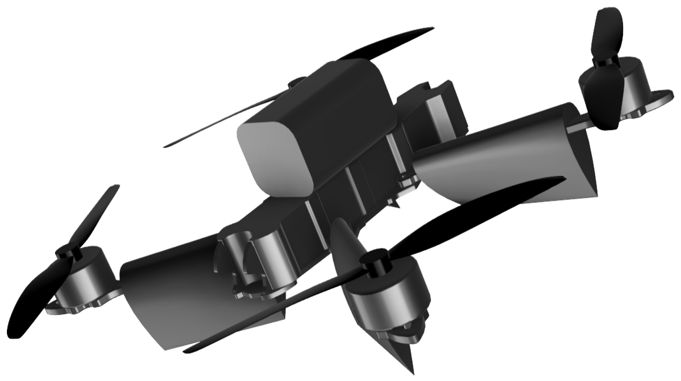
3. UAV Development—Standard Frame

This section focuses on the component selection and development of the standard frame UAV, designed to execute the mission previously outlined in Section 1.

3.1. UAV Propulsion Components

Table 1 outlines all the propulsion-related components chosen for the UAV under study, as well as the justification for each selection.
All the components listed in Table 1, along with the non-propulsion-related components such as the flight controller, GPS, video transmitter, optical flow sensor, and rangefinder, contribute to a total weight of approximately 1000 g. Despite the non-propulsion-related components being irrelevant to this study, they have to be accounted for in order to provide a total UAV weight estimate.
Figure 4 illustrates a simplified model of the standard frame UAV, created using components listed in Table 1. This model was designed in Autodesk Fusion 360 [43] CAD software and will be utilized in CFD simulations to analyze the aerodynamic forces acting on this frame.

3.2. eCal Performance Estimates

The eCalc Simulator, as previously mentioned in Section 2.2, was used to verify whether the selected components resulted in a well-performing multirotor. Only propulsion-related components were input into this simulator, including propellers, motors, ESCs, and battery. Data regarding the frame, such as its configuration (quadrotor) and size, were also provided. However, it is important to note that the simulator does not account for the frame’s aerodynamic properties, which largely explains the announced estimated error of approximately 15%.
Please note that this setup, which has an estimated weight of 1000 g, operates as a multirotor with conservative performance figures. It offers approximately 18 min of flight time and has a thrust-to-weight ratio at the suggested lower limit of 1.8, according to eCalc. Additionally, there are no issues related to power requirements or temperatures, as indicated by the simulation results in Figure 5.

4. UAV Improvement—Airfoil Frame

After developing the standard frame UAV, we explored ways to enhance its aerodynamic efficiency by incorporating airfoils into this frame, referred to hereafter as the airfoil frame. This section outlines the entire process of selecting and implementing the appropriate airfoils. It will also explain the CFD simulation analysis process used to theoretically determine whether this modification yields any improvements in performance.

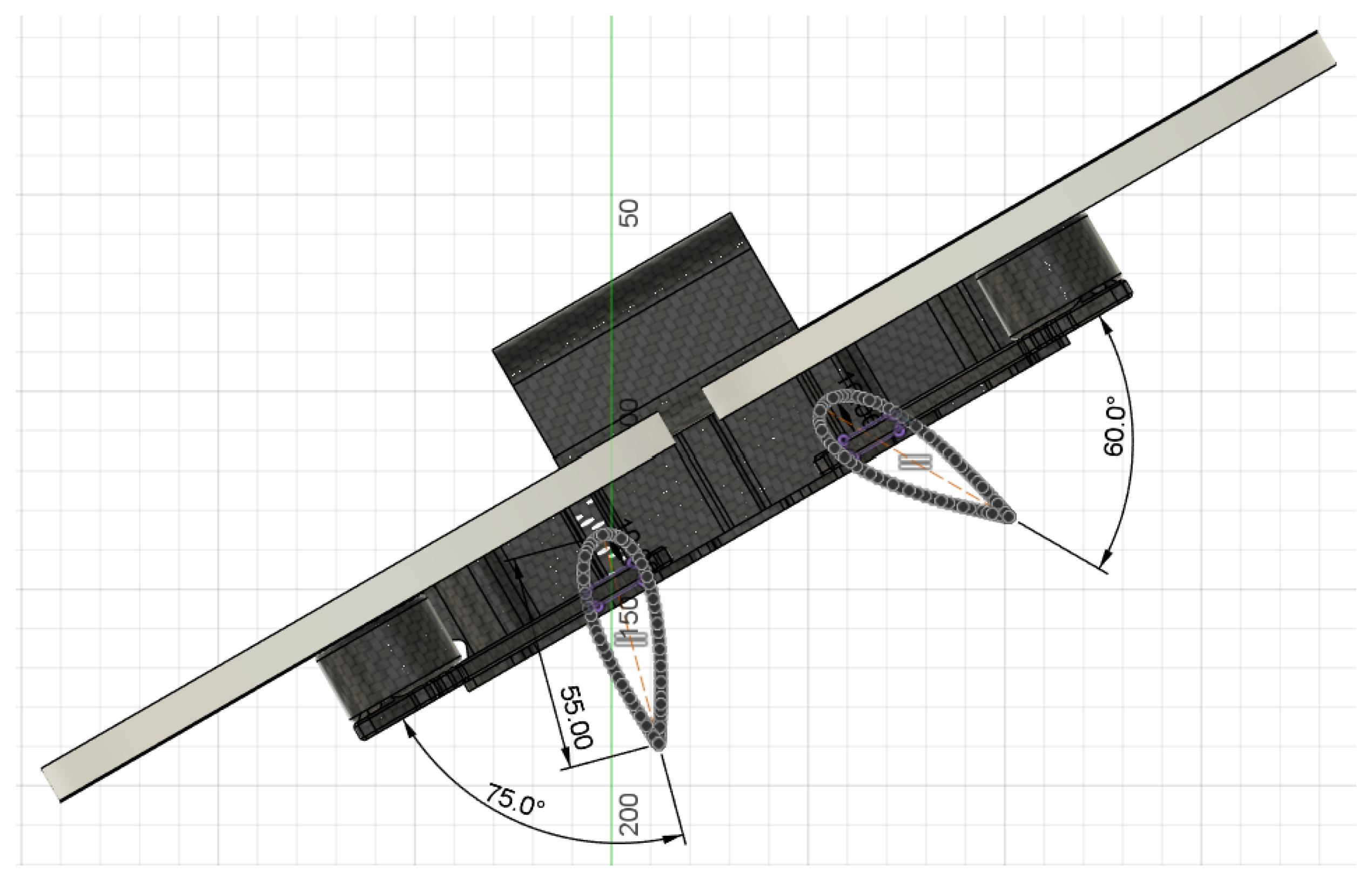
4.1. Simulated Flight Conditions

The first step involves modeling a frameless UAV, which consists solely of motors and propellers. The aim is to begin with a CFD simulation of this frameless design and subsequently conduct analyses using the standard and airfoil frames. This model’s simulation will serve to verify the reliability of the results obtained from the other simulations. Theoretically, the frameless model should achieve the highest forward thrust among the three tests, as incorporating a frame will naturally generate drag. Furthermore, this model is expected to produce the highest lift, unless the standard or airfoil frames generate additional lift due to the interaction of airflow with their surfaces.
Since the UAV under study is primarily designed for cruise flight, it is essential to begin with an analysis that simulates cruise flight conditions. These conditions involve horizontal flight at approximately constant speed and propeller RPMs. However, unlike airplanes, multirotors do not need to maintain a constant cruise flight, which means they frequently change flight conditions. Therefore, it was also necessary to study variations in flight speed and propeller RPMs to determine whether the airfoil frame can provide greater efficiency across all these scenarios.
Additionally, unlike airplanes, multirotors can hover in one place and perform vertical climbs and descents. After reaching their destination, multirotors often hover for extended periods. Therefore, while the modifications in this study are aimed at improving cruise flight, it is essential to ensure that they do not lead to significant performance trade-offs during hover flight. Ideally, it would be beneficial if the modifications also enhanced hover flight efficiency. To accomplish this, simulations should be performed with the UAV in a leveled position while varying external airflow and propeller RPMs. This approach will help assess different flight conditions, including hover, climb, and descent.

4.2. Airfoil Selection and Implementation

Firstly, to determine the best way to implement airfoils in the UAV frame, it is essential to study the aerodynamic behavior of the airflow around the standard frame, as well as the aerodynamic forces exerted on it.
Initial simulations of the standard frame were conducted at a target cruise speed of 20 m/s. The necessary propeller RPM value to maintain a steady altitude was found to be 20,000 RPMs. It is important to note that this value may not accurately reflect reality due to the 3D model of the propellers not being an exact representation of the actual ones. Nevertheless, as long as it is confirmed that the vertical component of the thrust produced is sufficient to balance the weight of the UAV (approximately 1000 g), the conclusions drawn from this study remain valid.
After conducting a flow visualization analysis, the simulation revealed that one of the primary sources of high downforce and drag in the standard frame is the low-pressure zones located below the frame arms, which can be observed in Figure 6 and Figure 7. These low-pressure areas are caused by flow separation at the edges of the arms. Therefore, adopting an airfoil shape for the frame arms could be an effective strategy to reduce flow separation, which would subsequently lower both downforce and drag.
Given the explanation in Section 2.3, reducing the downforce and drag created by the frame arms requires careful selection and orientation of the airfoil. The chosen airfoil must be aligned with the airflow around the arms and should have only enough thickness to cover the arm. For low tilt angles of the multirotor ( θ in Figure 8), the airflow around the arms, driven by the motor thrust, is primarily vertical. Therefore, the goal is to minimize the drag generated by the airfoils, as this drag translates into downforce (adding weight) relative to the frame’s movement.
Furthermore, since the airflow around the arms is roughly vertical, any lift produced by the airfoils (which acts perpendicular to the airflow direction) results primarily in drag in the frame’s reference of movement. It is essential, therefore, to ensure that the airfoils do not generate any lift. This can be achieved by selecting a symmetric airfoil and positioning it at an angle that results in zero AoA along the length of the arm.
Based on the flow visualization along the frame arms shown in Figure 6 and Figure 7, it can be concluded that if the airfoils are to align with the flow direction, the UAV arm will effectively act as a twisted wing.
However, it is important to note that the airflow over the UAV’s frame arm is not constant, as a multirotor continuously adjusts motor RPMs for flight control. Therefore, we have determined that the optimal airfoil choice for this frame is the NACA 0030 from the 4-Series family, as illustrated in Figure 9. The 4-Series airfoil family was selected because it offers several advantages (Appendix B) specifically suited for this application:
  • Simple geometry, which allows for easy manufacturing and modification;
  • Robust performance across various conditions;
  • Less sensitivity to surface imperfections compared to more advanced airfoils, making them suitable for 3D printing, which will be the method used for future real-world tests;
  • Predictable and gentle stall characteristics, resulting in a gradual loss of lift rather than a sudden drop, thus ensuring stability when the flow around the arms changes.
Among all the airfoils in the NACA 4-Series family, the 0030 was selected due to its advantageous features:
  • Thick airfoil design, more specifically 30% thickness, which not only covers the entire frame arm but also enhances structural strength;
  • Higher AoA before stalling compared to thinner airfoils, which is beneficial for this scenario because it helps to avoid flow separation and consequent extra drag;
  • A symmetrical shape, which is well suited for high Reynolds numbers, where turbulent flow is predominant, such as below UAV’s propellers. Additionally, the airfoil produces no pitching moment when the AoA is zero, ensuring consistent behavior, and it performs similarly whether the airflow is in a positive or negative AoA.
Despite the theoretical foundations defining the shape of a NACA 4-Series airfoil, as explained in Section 2.3.2, the CAD software used for modeling these UAVs includes scripts that can easily design an airfoil. Users simply need to provide a chord line and the corresponding airfoil coordinates in relation to that line in order to obtain the airfoil sketches, as illustrated in Figure 10 and Figure 11. The airfoil coordinates related to the chord line were generated using the Airfoil Tools generator [45]. This tool is capable of generating airfoil coordinates based on the shape parameters using the previously mentioned Equations (A1)–(A8). This process simplifies modeling the airfoil as a twisted wing with the correct angles of attack along the frame arm, aligning with the previously mentioned flow direction. This design can then be integrated into the standard frame, resulting in a new model known as the airfoil frame UAV (see Figure 12), which will be utilized in the CFD simulations. The aerodynamic forces acting on this frame, as determined by these simulations, will be compared to those measured on the standard frame.
Note that quadrotors, as other types of multirotors, have two propeller rotation configurations: propellers-in and propellers-out, as shown in Figure 13. There are several reasons for choosing one configuration over the other, which will not be discussed here.
The key point to note is that, in this study, the quadrotor operates in a propellers-out configuration, and if the user chooses to reverse the direction of rotation of the propellers and motors, all airfoil angles must be adjusted to achieve optimal aerodynamic performance. This necessity arises because reversing the propeller downwash flow alters the airflow around the quadrotor’s arms. This effect can be observed by comparing Figure 14 with Figure 6 and Figure 15 with Figure 7.
The main objective is to determine whether the wing-like arms can enhance the flight efficiency of the UAV. This will be assessed by comparing the total downforce and drag of the airfoil frame with that of the standard frame.
It is crucial that any potential decrease in downforce from the new frame is greater than the additional weight introduced to the UAV by the new wing-shaped components. To produce these components, the most straightforward and cost-effective manufacturing method for low production volumes is FDM 3D printing, as explained in Appendix C. With the 3D model file of these components and the slicer software, it becomes easy to obtain a highly accurate estimate of their weight by defining parameters such as wall layers, infill, and layer height.
Using Prusa Slicer software [47], the weight of the material required to print one wing using Polylactic Acid (PLA) was estimated with standard settings of 15% infill and a wall thickness of 2 perimeters. The estimated weight is approximately 20 g. Since the structural strength is primarily provided by the carbon arm, the wing can be made from a lighter material known as Lightweight-PLA. This material has been studied by researchers such as Bulota et al. [48] and Standau et al. [49]. Lightweight-PLA can reduce the weight of a standard PLA part by up to 40%, resulting in a new estimated weight of 12 g per wing, leading to a total added weight of 48 g for the four wings combined.

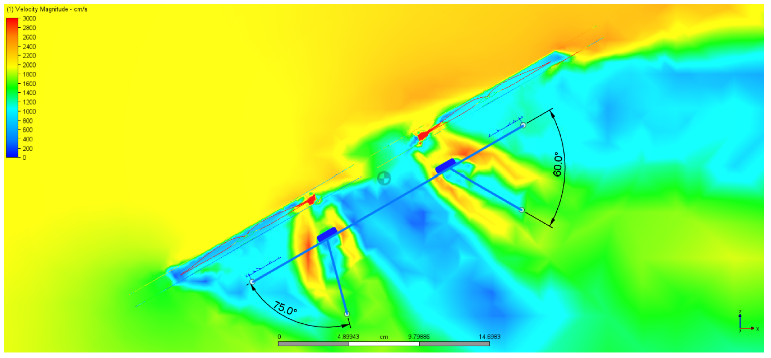
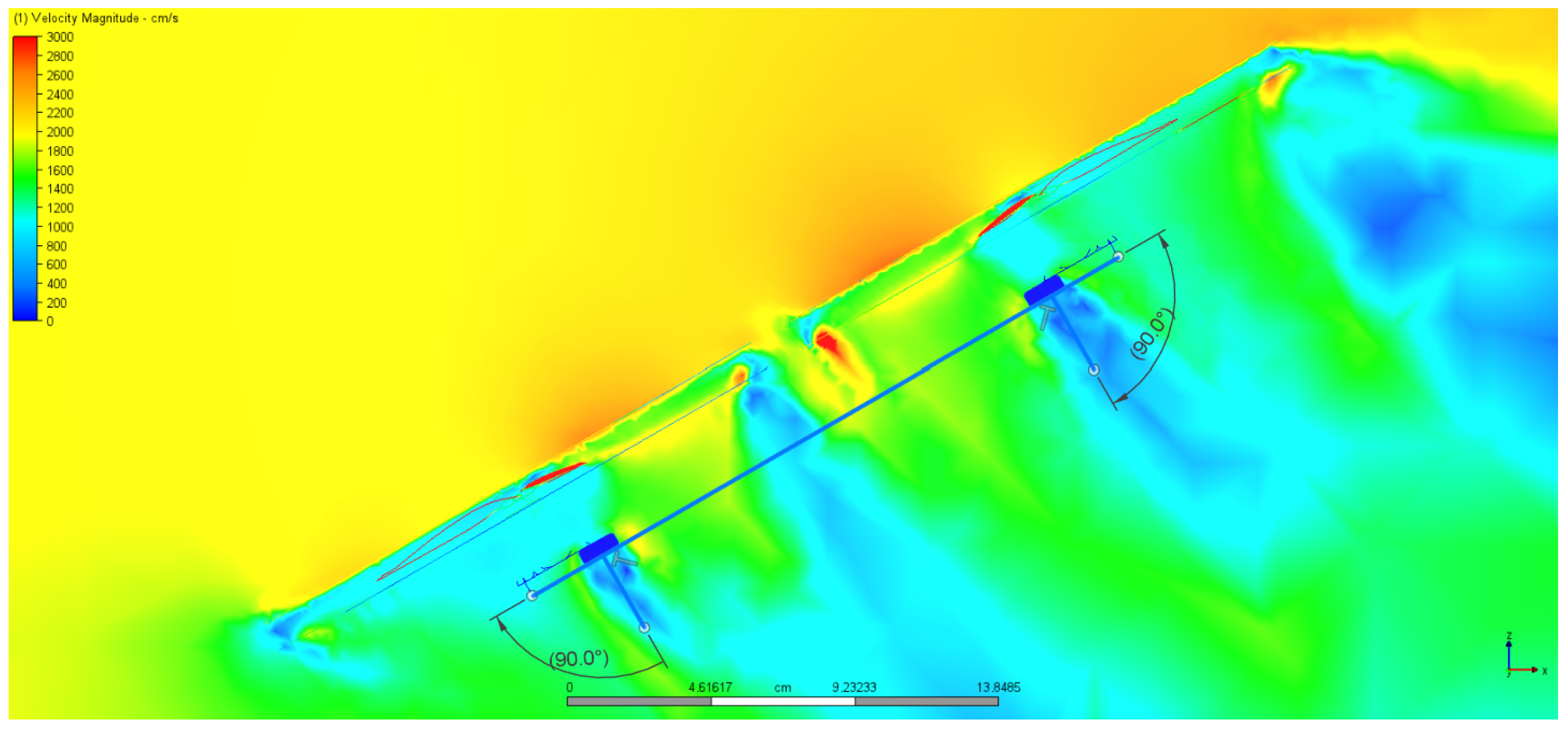
4.3. Airframe CFD Study Process Description

The results of this study were obtained using Autodesk CFD 2024 [36]. The tests were designed to simulate different flight modes of UAVs, including horizontal flight, hover flight, and vertical flight, while varying external airflow speed and motor RPMs. It is known that during UAV flight, the RPMs of the motors are not the same for each motor due to constant flight control adjustments. However, in this case, it is assumed that the motor rotations are equal, as these values are quite similar under steady flight conditions. Xiao et al. [50] used the same approximation in a similar research study.
The forces exerted on the UAVs during these tests will reveal the drag and lift forces each frame induces when compared to the frameless simulation.
Both the standard frame UAV and the airfoil frame UAV were modeled in CAD using Autodesk Fusion 360 [43] and subsequently placed within a designated volume of air to conduct an aerodynamic test, simulating conditions as if the UAVs were in a wind tunnel. This air volume was designed to be just large enough to prevent wall interactions with the airflow around the models. Note that, as mentioned in Section Process Description, a smaller external volume reduces the mesh size, which in turn decreases the simulation time.
To conduct the simulations, the material used for the propellers and motors was the default solid Acrylonitrile Butadiene Styrene (ABS). Since we are not focused on heat transfer properties, the specific material does not matter as long as it is solid. The material associated with the external volume was air with the default Autodesk settings, which simulates a flight at sea level with an ambient temperature of 19.85 ºC. The rotating motion of the propellers was implemented using the Rotating Region function of the software, with the rotation speed gradually increasing from 0 to 50 iterations, as recommended in the Autodesk CFD “Best Practices” documentation [51] for this type of simulation.
The boundary conditions were selected to simulate a test in a wind tunnel. For horizontal flight conditions, the inlet wall was configured for an orthogonal airflow with a constant speed, while the outlet wall was set to a constant zero relative pressure, simulating a free outlet of airflow. The walls parallel to the flow were all configured as Slip/Symmetry to avoid flow boundary layers that could interfere with the analysis.
In the case of hovering flight, the vertical walls were designated as Slip/Symmetry since they were parallel to the airflow. The top and bottom walls were set to maintain a constant zero relative pressure.
For vertical flight, the only modification from the hovering conditions was to introduce an orthogonal airflow inlet with constant speed on either the top or bottom wall, depending on whether the simulation represented a climb or a descent.
The mesh settings applied to the model were chosen based on the guidelines provided in the Autodesk CFD “Best Practices” documentation [51]. A sufficiently fine mesh density is crucial for a successful analysis, especially due to the high flow gradients present in a rotating device. However, an excessively fine mesh can hinder simulation completion time, so it is important to strike a balance that maintains result quality without being overly refined. The mesh sensitivity study addressed in Appendix D proves that the following steps generated a mesh capable of delivering accurate, reliable, and mesh-independent results.
The mesh distribution was defined using the Automatic Sizing feature, which generates a distribution based on the geometry’s curvature, specifically designed to create a smooth transition of mesh gradients across the entire model. A uniform setting was applied to the rotation region to avoid any artificial gradients in the flow caused by variations in mesh size.
Additionally, due to the turbulence model used in this simulation, which will be discussed later, it is necessary to incorporate wall layers into the mesh. This means adding elemental layers along all fluid–wall and fluid–solid interfaces, which enhances the original mesh and produces a smooth distribution along all walls, essential for accurate flow prediction. In this case, five layers were selected with a reduction thickness factor of 0.45 and automatic layer gradation. This choice allows for computational time savings and is supported by the results of the turbulence model verification in Appendix E.
For the solving process of the analysis, a transient analysis was selected with a time step determined by Formula (3).
t = D N × 6
where D = 360 / N u m b e r o f B l a d e s and N = B l a d e R P M . This is the recommended time step size for this simulation and propeller rotation, according to the software documentation. Additionally, for Rotating and Motion analyses, the advised number of inner iterations per time step is one. The SST k-omega turbulence model was chosen because it simulates turbulence all the way to the wall instead of using wall functions. It is recommended for external aerodynamics, separated or detached flows, and flows with adverse pressure gradients [52].
Furthermore, the option to enable Compressibility Effects of the Flow was selected. A fluid flow is considered compressible when its density varies with pressure. Compressible flows typically occur at high speeds, with Mach numbers greater than approximately 0.3. In the software being used, there is a distinction between subsonic compressible and fully compressible flows based on the Mach number [53].
Subsonic compressible flows have a Mach number between 0.3 and 0.8. In this range, the relationship between pressure and density is weak, and shock waves do not form within the flow. On the other hand, fully compressible flows have a Mach number greater than 0.8, where pressure significantly influences density, allowing for the possibility of shock waves.
Further classification identifies compressible flows as either transonic (Mach number between 0.8 and 1.2) or supersonic (Mach number between 1.2 and 3.0). In supersonic flows, changes in pressure effects are transmitted downstream; thus, upstream flow conditions are unaffected by any obstacles or conditions downstream.
The fastest moving part of a multirotor UAV is always the propeller tip. In this case, with 7-inch diameter propellers, a rotation speed of approximately 11,000 RPMs is sufficient to reach 0.3 Mach. Conversely, a rotation speed of approximately 29,500 RPMs is required to achieve 0.8 Mach. However, the UAV will not operate at such high rotational speeds. Therefore, it is reasonable to consider the flow in these simulations as compressible but subsonic.
Advection refers to the method of transporting a physical quantity, such as velocity or temperature, through a defined solution domain. In Autodesk CFD, five advection methods are available [54]. The method selected for our analysis is ADV 5 (Modified Petrov–Galerkin), which is the new default advection scheme. ADV 5 is a more stable variation of ADV 2, known as the Petrov–Galerkin advection scheme, which used to be the one recommended for pressure-driven flows, compressible flows, as well as scalar and energy transport equations and analyses involving rotating regions.
To determine the convergence of the analysis, it is essential that the changes in each degree of freedom over a wide range of iterations become minimized. The curves displayed in the Convergence Monitor of the software represent the average values of each degree of freedom throughout the entire calculation domain. It is established that if the lines in the Convergence Plot level off, the analysis is considered converged.
However, in transient analysis, since a transient flow does not reach a steady state, not all lines will flatten. Instead, they will oscillate around a consistent value. This behavior is illustrated in Figure 16, which depicts one of the analyses performed. Such oscillations indicate that the analysis has converged and the results can be addressed. Consequently, the number of time steps required for convergence varies depending on the specifics of each analysis. It was verified that, for these simulations, 2000 time steps would be enough to converge the analysis, which resulted in a simulated time of flight between 2.4 and 4 s, depending on the time step size.

5. Results

This section presents the results obtained from the CFD analysis for each of the flight conditions addressed.
As explained in the previous section, the steady horizontal forward flight at constant tilt was performed with the propeller’s RPMs maintained at a fixed value while varying the UAV’s flight speed. Next, the reverse test was conducted, where the flight speed and tilt of the UAV remained constant while the propeller RPMs were varied.
Finally, the leveled flight was examined. In this scenario, the UAV was kept horizontal, resulting in a null horizontal flight speed. The propeller RPMs were then adjusted to produce varying levels of thrust while maintaining a constant external airspeed. Additionally, the vertical airspeed was varied while keeping the propeller RPMs constant.

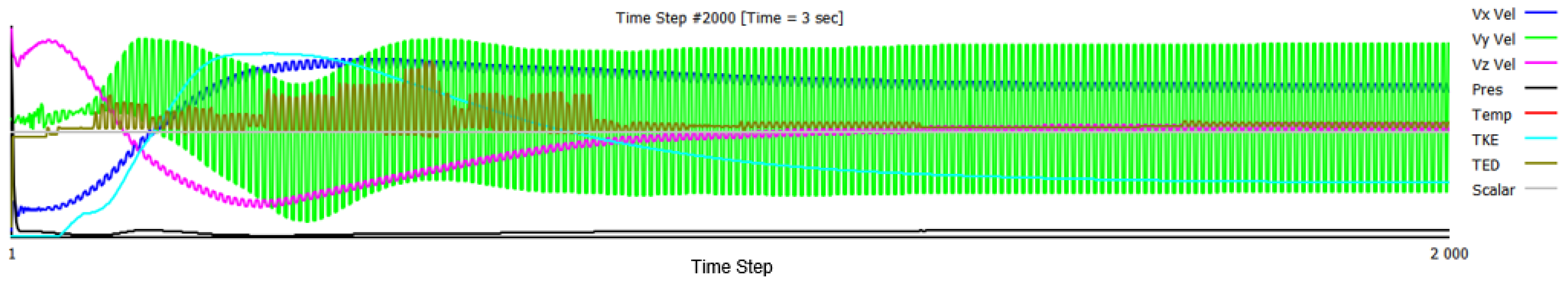
5.1. Processing of CFD Simulations Results

This subsection explains how to process the results from the simulations to extract useful data for comparing different frames. The simulations provide the total aerodynamic forces acting on the UAV due to the propeller’s rotation and the oncoming airflow. However, our focus is on the forces generated by the various types of frames. As previously mentioned, it is necessary to conduct three tests for each flight condition: frameless, standard frame, and airfoil frame. By comparing the results from each frame with those from the frameless simulation, we can estimate the drag and lift introduced by each frame.
As an example, we will consider the simulation with flight conditions of 20 m/s external airflow speed, 30-degree pitch (nose down), and propellers rotating at 20,000 RPMs. This serves as a representative case for all calculations performed. For other flight conditions, only the final results will be presented in tables, but the same calculations are applied.
Note that, in the following analysis, the multirotor is flying in the negative direction of the X-axis. This means that the X direction refers to the back, the Y direction refers to the right, and the Z direction refers to the top of the multirotor. This orientation also applies to the hover and vertical flight tests.

5.1.1. Frameless UAV

First, the frameless simulation (Figure 17) was analyzed, focusing only on the motors and spinning propellers. The resulting forces for this case are as follows:
  • F X 0 = −5.779 N (negative, meaning forward thrust);
  • F Y 0 = 0.003 N (approximately zero as expected due to the symmetry of the simulation);
  • F Z 0 = 10.420 N (positive, meaning upward thrust).

5.1.2. Standard Frame UAV

Next, the simulation was performed using the standard frame (Figure 18). The forces obtained for this case are as follows:
  • F X 1 = −4.223 N (negative, meaning forward thrust);
  • F Y 1 = −0.084 N (approximately zero as expected due to the symmetry of the simulation);
  • F Z 1 = 9.389 N (positive, meaning upward thrust).
To calculate the drag force caused by this frame ( F D 1 ), we need to compare the forces along the X-axis with those observed in the frameless simulation. In both scenarios, the forces are negative, indicating that, under these flight conditions, the UAV is attempting to accelerate forward. However, since the frameless case has a greater forward thrust than the standard frame, we can conclude that the standard frame introduces a drag value, as described by Equation (4).
F D 1 = F X 1 F X 0 = 4.223 ( 5.779 ) = 1.556 N
To calculate the drag coefficient of the standard frame ( C D 1 ), we use Equation (1) with the known values, as shown in (5).
C D 1 = 2 F D 1 ρ v 2 A F S F = 2 × 1.556 1.20473 × 20 2 × 0.012414837 0.520
Please note that the ρ value was selected for a flight at sea level, and the area considered was the frontal area of the standard frame UAV ( A F S F ) when moving forward at a defined tilt of 30 degrees.
In a similar manner to calculating drag force, the lift force induced by the standard frame ( F L 1 ) results from the comparison of the generated Z-axis forces against those from the frameless simulation. In both cases, these forces are positive, indicating that under these flight conditions, the UAV attempts to accelerate upwards. However, since the frameless configuration generates more upward thrust than the standard frame, we can conclude that the standard frame introduces a negative lift value, as given by Equation (6).
F L 1 = F Z 1 F Z 0 = 9.389 10.420 = 1.031 N
The negative lift value can be interpreted as downforce, which acts like Aerodynamic Added Weight (AAW) to the UAV. This additional weight requires more power to maintain altitude and perform flight maneuvers. This value is calculated using Equation (7).
A A W 1 = F L 1 g T = 1.031 9.807 0.1121 Kg = 105.1 g
where g T corresponds to the gravitational acceleration for objects near the earth’s surface.

5.1.3. Airfoil Frame UAV

For these flight conditions, the final simulation performed was the airfoil frame (Figure 19). The forces obtained for this case are as follows:
  • F X 2 = −3.818 N (negative, meaning forward thrust);
  • F Y 2 = −0.092 N (approximately zero as expected due to the symmetry of the simulation);
  • F Z 2 = 10.523 N (positive, meaning upward thrust).
Similarly to the previous case, to calculate the drag force induced by the airfoil frame, it is necessary to compare the X-axis forces with those from the frameless simulation. In both scenarios, the forces are negative, indicating that under these flight conditions, the UAV is attempting to accelerate forward. However, since the frameless case generates more forward thrust than the airfoil frame, it can be concluded that the airfoil frame also introduces drag, similar to the standard frame. Nonetheless, the drag value, as calculated using Equation (8), is higher, which indicates a deterioration in performance.
F D 2 = F X 2 F X 0 = 3.818 ( 5.779 ) = 1.961 N
It is also possible to calculate the drag coefficient of the airfoil frame ( C D 2 ) using Equation (1) and applying the known values, as shown in (9).
C D 2 = 2 F D 2 ρ v 2 A F A F = 2 × 1.961 1.20473 × 20 2 × 0.021265119 0.383
Similarly to the previous case, to calculate the lift force generated by the airfoil frame ( F L 2 ), it is necessary to compare the Z-axis forces between the airfoil frame and the frameless simulation. In both scenarios, the forces are positive, indicating that under these flight conditions, the UAV is attempting to accelerate upwards. However, in this case, the airfoil frame produces greater upward thrust than the frameless configuration. Therefore, we can conclude that the airfoil frame contributes a lift value as described by Equation (10).
F L 2 = F Z 2 F Z 0 = 10.523 10.420 = 0.103 N
This lift value can be understood as a negative AAW to the UAV. This indicates that, with this particular frame, the UAV requires less power to maintain these flight conditions, representing an improvement over the standard frame. This value is calculated using the Equation (11).
A A W 2 = F L 2 g T = 0.103 9.807 0.0105 Kg = 10.5 g

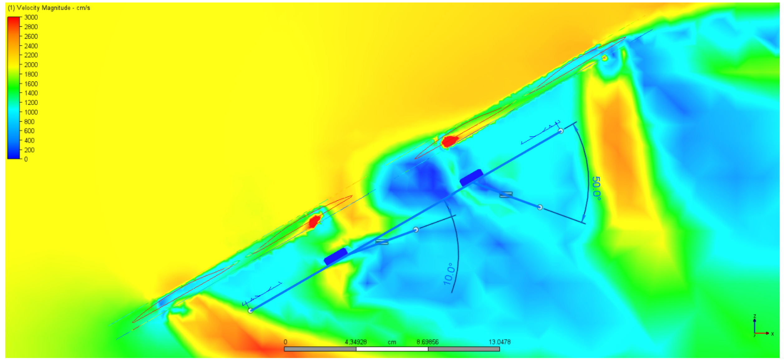
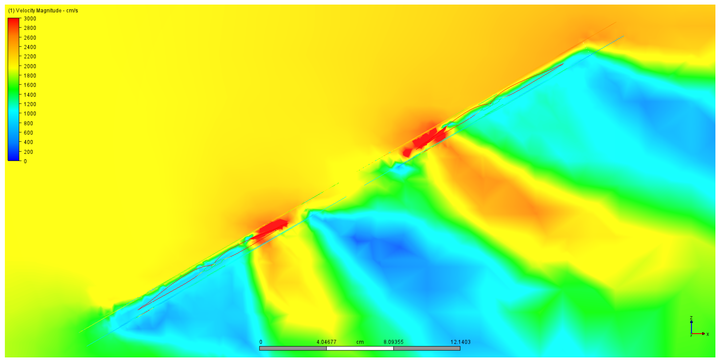
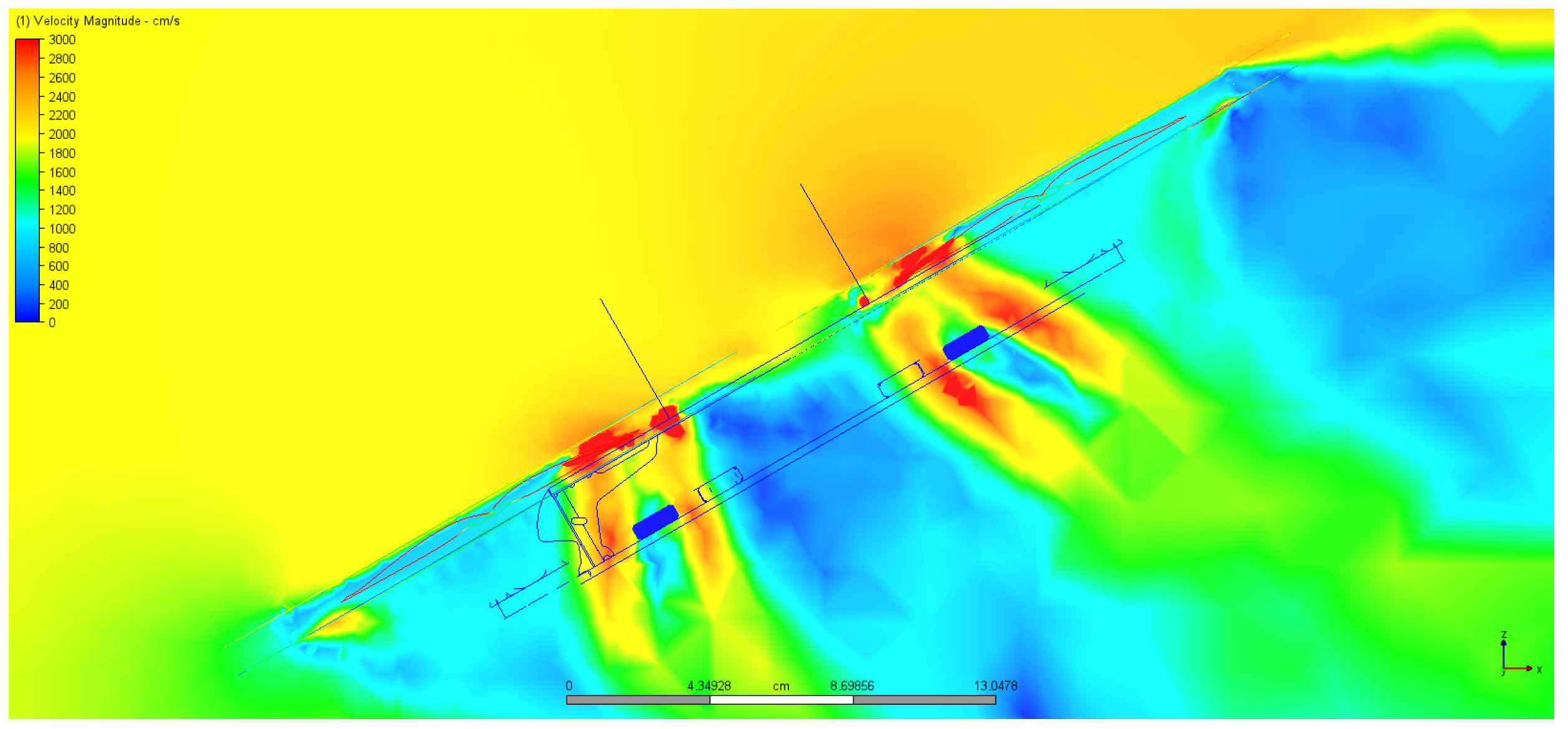
5.2. CFD Simulations and Processed Results

The tables in this subsection present the processed simulation results for all studied flight conditions, including the previously explained data. Note that the drag is not considered in leveled flight conditions because it can be viewed as downforce generated by the frame due to the vertical nature of the external airflow.

5.2.1. Horizontal Flight—Varying External Airflow Speed with Fixed Propeller Rotation

Table 2 presents the simulation results for horizontal steady flight at varying external airflow speeds with fixed propeller RPMs to simulate different flight speeds. This allows us to isolate and examine the impact of external airflow speed on the UAV’s aerodynamic performance.

5.2.2. Horizontal Flight—Varying Propeller Rotation with Fixed External Airflow

Table 3 presents the results of the simulations performed under horizontal steady flight conditions, where the propeller RPMs are varied while maintaining a constant external airflow. This enables us to isolate and study the effect of different thrust conditions on the UAV’s aerodynamic performance. The flight condition labeled “20 m/s External Flow Speed at 20,000 RPMs” is included again in this table to help illustrate the changes in forces as the motor RPMs alternate.

5.2.3. Leveled Flight—Varying External Airflow Speed with Fixed Propeller Rotation

Table 4 presents the simulation results for leveled flight, using fixed propeller RPMs while varying the external vertical airflow, enabling us to isolate and study its effect on the UAV’s aerodynamic performance.

5.2.4. Leveled Flight—Varying Propeller Rotation with Fixed External Airflow

Table 5 presents the simulation results for leveled flight under constant external airflow conditions and varying propeller RPMs, enabling us to isolate and study the effect of different thrust conditions on the UAV’s aerodynamic performance. To help illustrate how forces change with different thrust conditions, the “Steady External Flow at 20,000 RPMs” flight condition is also included in this table for clarity.

6. Simulation Result Analysis

In this section, we will discuss the CFD simulation results for the studied frames under various flight conditions. Additionally, we will analyze how these results may affect practical flight performance.
As previously mentioned, the frameless UAV simulation was used solely as a reference point to validate the results of the standard frame and airfoil frame simulations. To ensure the reliability of these results, some criteria must be met. First, the frameless UAV simulation should demonstrate the lowest drag among all simulations for each horizontal flight condition because there is no frame to generate the majority of the drag. Second, the standard frame simulations should exhibit higher downforce than the frameless UAV simulation during horizontal flight conditions, as the standard frame lacks lift surfaces. Finally, in vertical flight conditions, both the standard frame and airfoil frame should produce higher downforce than the frameless UAV simulation. In this scenario, horizontal drag is not considered since there is no horizontal movement.
Reviewing the data presented in the tables from Section 5, we can confirm that all these criteria were met for each flight condition, reinforcing the trustworthiness of the results.
All average values in this section’s tables were calculated assuming the UAV spends equal time in each studied flight condition between takeoff and landing.

6.1. Horizontal Flight—Lift/Downforce Analysis

The results from the horizontal steady flight simulations are presented in Table 2 and Table 3. As previously mentioned, these analyses intend to simulate the cruise flight conditions of the UAV, flying at a constant 30 degrees of tilt, at different speeds and motor RPMs.
The modifications made to the airfoil frame were anticipated to result in lower downforce compared to the standard frame, with the ideal outcome being a positive lift when compared to the frameless simulation. In fact, it was confirmed that, across all flight conditions (see Table 6), the airfoil frame consistently generated positive lift. This indicates that the addition of airfoils to the frame arms not only eliminates the downforce created by the standard frame but also contributes with lift, resulting in improvement values above 100%. Furthermore, it is noteworthy that as external airflow speed or propeller thrust increases, the downforce of the standard frame rises, while the lift produced by the airfoil frame remains relatively constant. In conclusion, the airfoil frame demonstrated an average lift improvement of 118% compared to the standard frame.
As discussed in Section 5.1, the difference in lift and downforce generated by each frame can be translated into an AAW for the UAV during horizontal flight. Thus, in Table 7, which presents the AAW results, we can observe the same trends as those noted in Table 6, but this time the data are represented in units of grams.
By adding the AAW to the original weight of the UAV, we can obtain an approximate estimate of the momentary weight that the propellers must support considering the studied flight conditions (see Table 8). The UAV’s original weight is considered to be 1000 g (as noted in Section 3.2), while the weight of the additional airfoils is approximately 48 g (discussed in Section 4.2). As anticipated due to previous results, the airfoil frame’s momentary weight remains relatively constant, while the standard frame’s fluctuates with varying flight conditions, increasing with either external airflow or propeller thrust increments. In summary, the airfoil frame achieved an average momentary weight reduction of 6.5% across the studied flight conditions.
Finally, it is possible to use the eCalc Simulator to obtain an estimate of the impact of these changes in the total flight time in the studied conditions. For this estimate, the momentary weight of each UAV was used as its total weight, and the Mixed Flight Time Estimate of eCalc with 85% of battery capacity used was considered as a safe margin. The results in Table 9 indicate that the airfoil frame achieved an average increase in flight time of 7.6% across the various flight conditions studied. Additionally, the data show that as speed and thrust increase, the efficiency of the airfoil frame becomes significantly more pronounced compared to the standard frame.

6.2. Horizontal Flight—Drag Analysis

In terms of drag, it was anticipated that the airfoil frame would at least maintain a drag value comparable to that of the standard frame, with the ideal scenario being a lower drag value. However, this expectation was not met. As shown in Table 10, for most of the flight conditions examined, the airfoil frame exhibited a higher drag value than the standard frame, with an average increment of 22.9%.
In terms of drag coefficient, this value should remain relatively constant as long as the simulation conditions do not change significantly regarding flow speed, flow direction, object position, object size, fluid density, or fluid viscosity. Therefore, it was anticipated that the drag coefficient would stay approximately constant across all studied flight conditions for both frames. This expectation was confirmed for the airfoil frame, but not for the standard frame, as shown in Table 11. This discrepancy may be attributed to the increased flow separation occurring beneath the arms of the standard frame, leading to greater turbulence and unpredictability in the flow. Interestingly, despite having a higher total drag, the airfoil frame exhibits a lower drag coefficient compared to the standard frame. This demonstrates the aerodynamic efficiency of the airfoil shapes when assessed against the frontal area that these increase on the frame.
Based on these results, we can observe that incorporating airfoils into the arms of a standard UAV frame presents a trade-off during horizontal flight conditions. While this design can lead to improved efficiency in the vertical direction, it tends to reduce performance in the horizontal direction. Practically, this means longer flight times but lower top speeds and reduced wind resistance.
To estimate how much the top speed of the airfoil frame may be reduced, we can analyze the sum of the external forces acting on the UAV in the horizontal axis, following a specific calculation process:
T X m a x D = m a
where the following are true:
  • T x m a x —horizontal component of the maximum UAV propellers’ thrust;
  • D—drag of the UAV;
  • m—mass of the UAV;
  • a—acceleration of the UAV.
Since, at top speed ( V m a x ), the acceleration is null, we have:
T x m a x = D T x m a x = 1 2 ρ C D A F V m a x 2 V m a x = 2 T x m a x ρ 1 C D A F
Since T x m a x and ρ are constant, we have:
V m a x = K 1 C D A F
where K = 2 T x m a x ρ is a constant. Additionally, remember that the drag coefficients of the airfoil frame ( C D A F ) and the standard frame ( C D S F ), as well as their frontal areas ( A F A F and A F S F ), were previously mentioned, so we have:
C D A F C D S F = 0.384 0.549 = 0.70
A F A F A F S F = 0.021265119 0.012414837 = 1.71
V m a x A F = K 1 0.70 C D S F × 1.71 A F S F = 1 0.70 × 1.71 × K 1 C D S F A F S F
V m a x A F = 0.914 × V m a x S F
Thus, it is concluded that the horizontal top speed of the airfoil frame is approximately 96% of the standard frame.
In summary, if the UAV spends an equal amount of time in each of these horizontal flight conditions, incorporating airfoils in the arms of a standard UAV frame will result in an average improvement of 7.6% in flight times, accompanied by a 8.6% reduction in top speed. The decision regarding whether this trade-off is suitable for the mission will depend on the UAV’s intended purpose and the operator’s expectations.

6.3. Leveled Flight—Lift/Downforce Analysis

The results from the leveled flight simulations are present in Table 4 and Table 5. These analyses intend to simulate hover and vertical flight conditions by varying external vertical airflow speed and propeller RPMs.
The modifications made to the airfoil frame were aimed at enhancing aerodynamic efficiency during horizontal flight, as previously mentioned. However, during hover and vertical flight, there is no horizontal external airflow to aid in lift generation. Therefore, it is crucial to assess whether the airfoil-shaped arms can reduce drag in the vertical direction, which translates to downforce from the UAV’s perspective. It was confirmed that, across all flight conditions (see Table 12), the airfoil frame consistently produced significantly less downforce compared to the standard frame, presenting an average of 43.3% improvement.
As previously discussed, this difference in downforce generated by each frame can be translated into AAW for the UAV during these leveled flight conditions. Thus, in Table 13, we can observe the same trends as those noted in the previous table, but this time the data are represented in units of grams.
Following a similar approach to the previous analyses, we can estimate the momentary weight that the propellers must support under the studied flight conditions by adding the AAW to the original weight of the UAV (see Table 14). Remember that the UAV’s original weight is considered to be 1000 g, while the weight of the additional airfoils is approximately 48 grams.
In this case, it is noticeable in certain flight conditions, such as lower-propeller RPMs, that the additional weight of the airfoils nearly negates all the aerodynamic benefits they provide.
Additionally, in the previous analysis of horizontal flight, we observed that the airfoil frame’s momentary weight remained relatively constant across all flight conditions. However, during leveled flight, we noticed that the momentary weight of the airfoil frame increased with either faster-descending external airflow or increased propeller thrust. Despite these variations, it remained quite similar to the standard frame’s momentary weight, only presenting a 2.6% reduction.
To evaluate the impact of these changes on flight time under the studied conditions, we can use the eCalc Simulator once again. Similar to the previous analysis, we considered the momentary weight of each UAV as its total weight and relied on the hovering flight time estimates provided by eCalc. The results presented in Table 15 indicate that the airfoil frame achieved an average flight time increase of 4.6% across the examined flight conditions. This increase is particularly pronounced at higher-propeller RPMs or in stronger-ascending external airflow, indicating that UAVs with higher thrust during hovering (heavier UAVs) take more benefit from airfoil-shaped arms.

6.4. Leveled Flight—Horizontal Forces Analysis

While it may not be a major topic of discussion, we also decided to address the effects of horizontal forces when the UAV is hovering or flying vertically.
Due to the longitudinal and transversal symmetry of standard frame UAVs, we anticipated that no horizontal aerodynamic forces would occur under any leveled flight conditions. This expectation was confirmed in Table 16 for the longitudinal direction and Table 17 for the transversal direction, where it is noticeable that the average values are very approximate to zero.
In the case of the airfoil frame UAV, it was found that a significant force was generated in the negative X-axis direction (toward the front of the UAV) under all flight conditions. This longitudinal force arises from a slight difference between the tilt/twist angle of the forward and backward airfoils, which disrupts the longitudinal symmetry of the frame. However, there is no such difference between the left and right airfoils, allowing for the maintenance of transversal symmetry. As a result, the horizontal forces acting along the Y-axis are much closer to zero, similar to those observed in a standard frame.
This characteristic of the airfoil frame UAV presents as a disadvantage compared to the standard frame. When hovering, the airfoil frame UAV must tilt slightly backwards to counteract its natural tendency to move forward, which can reduce hover flight efficiency. A straightforward solution to this issue would be to design the front and back airfoils to be symmetrical, which would tailor the UAV for hovering.

7. Conclusions

This study demonstrated the feasibility of integrating airfoil shapes into the frame arms of multirotor UAVs to enhance their aerodynamic performance.
By redesigning traditional quadrotor frames into airfoil-equipped configurations, a considerable reduction in downforce was observed through comprehensive CFD simulations, translating into improved energy efficiency and extended flight durations. However, the integration of airfoil shapes led to a slight increase in drag due to the additional surface area and structural modifications.
Despite this drawback, the overall efficiency of the airfoil-integrated frame was found to be superior in various flight conditions, particularly in cruise scenarios where the reduction in downforce significantly eased the load on the motors, extending flight duration. These findings highlight the potential for such design innovations to improve the operational capabilities of multirotors, particularly for missions requiring extended endurance and efficiency.
To summarize, the main contributions of this research are as follows:
  • Demonstrated that modifying UAV arms with airfoil shapes can enhance aerodynamic efficiency without major structural changes;
  • Provided a comparative evaluation of a standard quadrotor frame and an airfoil-integrated design through CFD-based aerodynamic analysis, highlighting differences in drag and downforce;
  • Showed that airfoil arms significantly reduce downforce, leading to lower effective weight on the motors and reducing overall power consumption;
  • Proposed a systematic approach to incorporating airfoil structures into UAV frames while maintaining structural simplicity and manufacturability.
  • Highlighted how airfoil-integrated UAVs could benefit fields such as military reconnaissance, agriculture, and industrial inspections, where extended flight duration is critical.
Overall, this innovative approach opens avenues for future research focusing on practical implementation by wind tunnel and real flight tests, as well as the exploration of advanced materials to reduce weight and optimization for specific mission profiles. This study underscores the importance of aerodynamics in UAV design and provides a solid foundation for integrating efficient structural solutions into multirotor UAVs.

Author Contributions

Conceptualization, A.A.C.F.; Formal analysis, A.A.C.F.; Funding acquisition, R.M.A.C.; Investigation, A.A.C.F. and V.W.G.A.; Methodology, A.A.C.F.; Project administration, R.M.A.C.; Supervision, R.M.A.C.; Validation, A.A.C.F.; Visualization, V.W.G.A.; Writing—original draft, A.A.C.F.; Writing—review and editing, V.W.G.A., V.H.A.A., J.M.A.L., and R.M.A.C. All authors have read and agreed to the published version of the manuscript.

Funding

This research was funded by Estado-Maior-General das Forças Armadas (EMGFA). The APC was funded by Agência Regional para o Desenvolvimento da Investigação, Tecnologia e Inovação (ARDITI).

Institutional Review Board Statement

Not applicable.

Informed Consent Statement

Not applicable.

Data Availability Statement

The raw data supporting the conclusions of this article will be made available by the authors on request.

DURC Statement

Current research is limited to the field of aerospace engineering and focuses on improving the aerodynamic performance of multirotor UAVs, enabling increased flight time and range, which is beneficial to the entire multirotor UAV development industry and does not pose a threat to public health or national security. The authors acknowledge the dual-use potential of the research involving increased-range multirotor UAVs and confirm that all necessary precautions have been taken to prevent potential misuse. As an ethical responsibility, the authors strictly adhere to relevant national and international laws about DURC. The authors advocate for responsible deployment, ethical considerations, regulatory compliance, and transparent reporting to mitigate misuse risks and foster beneficial outcomes.

Conflicts of Interest

The authors declare no conflicts of interest.

Appendix A. UAV Propulsion-Related Components

This appendix offers a concise overview of each UAV propulsion-related component and outlines key specifications to consider for a thoughtful component selection.

Appendix A.1. Frame

One of the first and most important steps in developing a multirotor is selecting an appropriate frame configuration and size. Multirotors are generally categorized by the number of motors they use, including Bicopters (two motors), Tricopters (three motors), quadrotors (four motors), Hexacopters (six motors), and more. Each of these configurations can be built using different frame designs, as noted by Liang [55].
Comparing different multirotor categories of the same size reveals that the number of motors and the frame configuration significantly affect flight performance. Each configuration has its own advantages and disadvantages. Generally, a multirotor with fewer motors can accommodate longer propellers within the same size constraints. Larger propellers enhance efficiency, providing more thrust for the same amount of power, which leads to longer flight times. However, using larger propellers necessitates bigger motors, which adds weight and requires a more powerful battery and electronics. This combination results in a greater moment of inertia, making the multirotor less responsive. On the other hand, if a multirotor has three or fewer motors, it will require additional actuators and/or control surfaces to achieve flight in addition to the motors. These actuators are typically servos, which are more affordable than brushless motors. However, servos are less robust and have slower response times, often resulting in decreased flight stability, which can become a vulnerability, as noted by Liang [55].
A multirotor with more motors typically can accommodate shorter propellers within the same size constraints. However, having additional motors increases thrust and lifting capacity while also enhancing redundancy. This means that if one motor fails, the UAV can still maintain stability, allowing for a safe landing as referred to by Achtelik et al. [56].
According to Toglefritz [57], the quadrotor is the most popular multirotor configuration in the industry because it provides the best balance between the advantages and disadvantages of various multirotor types. Additionally, Bondyra et al. [58] noted a growing interest in the octocopter X8 configuration for larger UAVs. This configuration features a traditional quadrotor design with two motors per arm.

Appendix A.2. Propellers

Propellers are the components that generate the thrust needed to keep multirotors airborne and allow them to maneuver in various directions. According to Theys et al. [59], selecting the appropriate propellers for each multirotor is vital, since this can significantly reduce noise while enhancing flight time, speed, and lifting capacity, depending on the user’s goals. Various factors influence the performance of drone propellers, including pitch, shape, and the number of blades.
According to Liang [60], propellers are designed to spin either clockwise (CW) or counter-clockwise (CCW). In a typical multirotor setup, an equal number of motors rotate in the CW and CCW directions to maintain stability around the yaw axis. Therefore, it is crucial to match the propellers to the motors according to their intended direction of rotation.
The length of a propeller refers to the diameter of the circular disc it creates when spinning. With a constant pitch and the same number of blades, a longer propeller can generate more thrust because it increases the surface area. This allows a multirotor to accelerate faster and hover at lower rotations per minute (RPMs), which results in decreased noise levels. The same principle applies to propellers with a higher number of blades. However, using longer or more-bladed propellers requires more power from the motor.
It is important to note that while longer propellers can improve acceleration, they do not necessarily lead to higher top speeds, as acceleration and maximum speed are distinct concepts. In contrast, shorter propellers or those with fewer blades can spin up and slow down more quickly due to reduced drag from tip vortices and lower moments of inertia. This characteristic makes the multirotor more agile and responsive, as suggested by Kovtun [61].
The pitch of a propeller refers to the distance it would travel in one complete revolution if it were moving through a solid medium instead of air. A propeller with a higher pitch generates more thrust when the multirotor is flying at high speeds, allowing for a greater top speed. However, it creates less thrust when the multirotor is hovering and produces more turbulence and prop wash, which adversely affects the efficiency of the UAV. Additionally, a higher pitch causes the propeller to spin more slowly, making the multirotor less responsive. These pitch-related performance changes in propellers were addressed by Podsedkowski et al. [62] during their development of a variable-pitch propeller for experimental UAV tests.
According to Ramesh et al. [63], the weight of a propeller is another crucial factor to consider. Propellers with lower moments of inertia tend to perform better, as they subject the motor to less torque loading, enable faster spool-up times, and enhance overall performance and responsiveness. To achieve a lower moment of inertia, a propeller must have blades with the center of mass closer to the hub and generally lower weight. However, this design can lead to thinner blades, which makes them more susceptible to breakage. Finally, Liang [60] provided a useful guide for selecting appropriate propellers based on the specific goals of the multirotor.

Appendix A.3. Motors

Müller [20] emphasizes that before selecting a motor for a multirotor UAV, it is essential to estimate the intended size and weight of the vehicle. By determining the frame size, the maximum propeller size can be established. While the weight estimate does not need to be extremely precise, a more accurate estimate generally leads to better UAV performance. It is advisable to err on the side of overestimation of the weight to ensure that there is sufficient power available, rather than underestimating it, which could result in difficulties during climbs and fast maneuvers.
Putra et al. [64] suggest that the maximum thrust generated by all motors should ideally be at least double the total weight of the multirotor. However, this guideline may vary depending on the desired maneuverability. Insufficient thrust may lead to poor control responses and difficulties during takeoff. Having more thrust available than necessary can be beneficial for carrying additional payloads and improving control at high speeds. However, this increased thrust may also result in decreased efficiency and, consequently, shorter flight times.
According to Uçar et al. [65], the most crucial factors to consider when choosing a motor are weight, power (thrust), operating voltage, operating current, torque, and KV.
“KV” refers to the number of RPMs a motor produces when 1 volt is applied without any load attached. Pairing a high-KV motor with an excessively large propeller can create problems, as the motor will attempt to spin at the same speed as if it were mounted with a smaller propeller. This increased demand for torque results in a higher current draw and generates more heat, which can lead to overheating or even motor burnout. Therefore, as supported by Bershadsky et al. [66], it is essential to choose the motor KV, along with other motor specifications, carefully. Generally, larger propellers are best matched with low-KV motors, while high-KV motors work more effectively with smaller and lighter propellers.

Appendix A.4. Electronic Speed Controller

Bershadsky et al. [66] explain that Electronic Speed Controllers (ESCs) are responsible for regulating the speed of UAV brushless motors. These operate using direct current (DC) supplied by the battery and receive throttle signals from the flight controller, providing three-phase alternating current (AC) to the motor and enabling it to run at the desired speed. Utilizing high-quality ESCs significantly enhances the reliability and smoothness of the flight experience.
Liang [67] discusses both single and four-in-one configurations. Single ESCs are known for their ease of use and cost-effectiveness because they can be replaced individually if damaged. However, they do have some drawbacks, including the need for more soldering and wiring. This can lead to a slightly heavier drone due to the added weight of additional wires and a power distribution board.
On the other hand, four-in-one ESCs combine four individuals into a single circuit board, each controlling its own motor. If one fails, the entire board must be replaced. Fortunately, modern ones are highly reliable, so this is generally not a significant concern.
To choose the right ESC for a UAV, it is essential to verify that it is compatible with both the battery’s voltage and the maximum current draw of the selected motors. Additionally, some users may want to consider the firmware that runs on these boards, as certain versions may have limitations regarding features and protocols.

Appendix A.5. Battery

The battery is the power source for the UAV, and, according to Delbecq et al. [68], its selection is influenced by various factors such as the UAV’s specifications and flight requirements.
According to Liang [69], it is crucial to determine the appropriate voltage and capacity of the battery, ensuring compatibility with the UAV components and the intended flight objectives. Batteries with a higher voltage provide more power, while those with a higher capacity enable longer flight times. Additionally, it is recommended to choose batteries with a higher discharge rating (C-rating) to ensure they can deliver the necessary current required by the motors during maneuvers. Finally, it is important to consider the battery’s weight and size to maintain the desired thrust-to-weight ratio of the UAV.

Appendix B. NACA Airfoil Families

The first series of NACA airfoils, which include the 4-Digit, 5-Digit, and modified 4/5-Digit models, was developed using analytical equations. These equations describe the camber (curvature) of the mean line (the geometric center line) of the airfoil section, as well as the thickness distribution along the length of the airfoil (see Figure A1). Later-developed airfoil families feature more complex shapes derived from theoretical methods rather than purely geometrical approaches. The following information about NACA airfoils is provided by Leishman et al. [70].
Figure A1. NACA method for defining shape of airfoil. Illustration by Leishman [70].
Drones 09 00202 g0a1
The first family of airfoils designed using this method is known as the NACA 4-Digit Series. In this system, the first digit indicates the maximum camber (m) of the airfoil, the second digit specifies the position of the maximum camber (p), and the last two digits represent the maximum thickness (t), all expressed as a percentage of the chord length. The coordinates of the mean camber line for the airfoil can be calculated by substituting the values of m and p into Equations (A1) and (A2) for each x coordinate.
y c = m p 2 ( 2 p x x 2 ) , f r o m x = 0 t o x = p
y c = m ( 1 p ) 2 [ ( 1 2 p ) + 2 p x x 2 ] , f r o m x = p t o x = c
where the following are true:
  • x = coordinate along the length of the airfoil, from 0 to c (which stands for chord length);
  • y c = camber coordinates.
The thickness distribution above and below the mean line ( y t ) can be determined by substituting the value of t into Equation (A3) for each x coordinate.
y t = t 0.2 ( 0.2969 x 0.1260 x 0.3516 x 2 + 0.2843 x 3 0.1015 x 4 )
The final coordinates for the airfoil upper surface ( x U , y U ) and lower surface ( x L , y L ) are obtained using the following equations.
x U = x y t sin θ
y U = y c + y t cos θ
x L = x + y t sin θ
y L = y c y t cos θ
where θ , defined by the following formula, corresponds to the camber-line angle.
θ = arctan ( d y c d x )
The naming convention for the NACA 5-Digit Series is slightly more complex. The first digit, when multiplied by 3/20, represents the design lift coefficient. The next two digits, when divided by 20, indicate the position of the maximum camber as a percentage of the chord. The final two digits represent the maximum thickness, also expressed as a percentage of the chord. The NACA 5-Digit Series employs the same thickness formulas as the 4-Digit Series. However, the mean camber line is defined by a different equation.
NACA 4- and 5-Digit Series airfoils can be modified using a two-digit code that is preceded by a hyphen. The first digit indicates the roundness of the leading edge: a value of 0 signifies a sharp edge, 6 means the airfoil maintains its original shape, and larger values indicate a more rounded leading edge. The second digit, multiplied by 10, specifies the distance of maximum thickness from the leading edge as a percentage of the chord. Additionally, all numbers can be expressed as decimals for a more precise description of the airfoil.
The NACA 1-Series, also known as the 16-Series, was developed based on airfoil theory rather than geometrical relationships, which distinguishes it from other airfoil families. The fundamental idea behind this design approach is to define the desired pressure distribution over the airfoil and then create a geometrical shape that achieves that distribution. Since the 16-XXX airfoils have been the most widely used from this family, it is often referred to as the 16-Series rather than simply as a subset of the 1-Series.
The NACA 6-Series was developed using an advanced theoretical method similar to the 1-Series. This method involved specifying a desired pressure distribution and using complex mathematics to determine the necessary geometrical shape of the airfoil. The objective was to design airfoils that maximize the area over which airflow remains laminar. By doing so, the drag can be significantly reduced across a small range of lift coefficients.
The NACA 7-Series aimed to optimize laminar flow regions over an airfoil by differentiating the locations of minimum pressure on the upper and lower surfaces.
The NACA 8-Series represents a final variation of the 6- and 7-Series designs, specifically intended for flight at supercritical speeds. The primary goal of this series was to maximize the extent of laminar flow on both the upper and lower surfaces of the airfoil independently. The thickness distribution and camber of an airfoil play crucial roles in how much air accelerates around it. As the speed of airflow approaches the speed of sound, it can reach Mach 1, leading to the formation of shock waves, which create wave drag. Supercritical airfoils are engineered to minimize this wave drag effect by featuring a flatter upper surface.
After mentioning the existing NACA airfoil families, it is essential to explore the advantages, disadvantages, and applications of each one. These are summarized in Table A1, provided by Scott [71].
Table A1. Summary of NACA airfoil families’ advantages, disadvantages, and applications according to Scott [71].
FamilyAdvantagesDisadvantagesApplications
4-Digit1. Good stall characteristics
2. Small center of pressure movement
across large speed range
3. Roughness has little effect
1. Low maximum lift coefficient
2. Relatively high drag
3. High pitching moment
1. General aviation
2. Horizontal tails
Symmetrical:
3. Supersonic jets
4. Helicopter blades
5. Shrouds
6. Missile/rocket fins
5-Digit1. Higher maximum lift coefficient
2. Low pitching moment
3. Roughness has little effect
1. Poor stall behavior
2. Relatively high drag
1. General aviation
2. Piston-powered
bombers, transports
3. Commuters
4. Business jets
16-Series1. Avoids low-pressure peaks
2. Low drag at high speed
1. Relatively low lift1. Aircraft propellers
2. Ship propellers
6-Series1. High maximum lift coefficient
2. Very low drag over a small range
of operating conditions
3. Optimized for high speed
1. High drag outside of the optimum
range of operating conditions
2. High pitching moment
3. Poor stall behavior
4. Very susceptible to roughness  
1. Piston-powered fighters
2. Business jets
3. Jet trainers
4. Supersonic jets
7-Series  1. Very low drag over a small range
of operating conditions
2. Low pitching moment
1. Reduced maximum lift coefficient
2. High drag outside of the optimum
range of operating conditions
3. Poor stall behavior
4. Very susceptible to roughness
Seldom used
8-SeriesUnknownUnknownVery seldom used

Appendix C. Manufacturing Process

Although this study does not focus on UAV manufacturing or practical tests, it is essential to understand how the improved frame can be produced. This knowledge will help estimate its weight and allow for a comparison with the thrust predicted by theoretical analysis.
According to Mohamed et al. [72], Fused Deposition Modeling (FDM) is an advanced 3D printing and additive manufacturing technique that utilizes plastic materials. It is widely appreciated for its accessibility, prototyping accuracy, and low cost. Chennakesava et al. [73] and Rajan et al. [74] explain that FDM creates 3D structures through the melt-extrusion of a plastic filament and the steps of this procedure.
The process begins with generating a digital design of the object using 3D design software. This model is then converted into a G-code format, typically through slicer software, which is a process that translates the design into machine-readable instructions. Finally, the printer executes the G-code, building the model layer by layer until the complete object is produced. It is important to note that the G-code is the script that directs the printer’s actions throughout this process.
The main advantages of FDM manufacturing include the ability to produce complex parts with good accuracy at a lower cost compared to conventional manufacturing processes, as addressed by Zhao et al. [75]. Additionally, this process does not require special tooling.
However, there are some disadvantages to consider. The costs can become high for large-scale production, the size of the output is limited by the printer bed dimensions, there are restrictions on the types of raw materials that can be used, and this is still an evolving technology that may necessitate a considerable level of expertise from the user.
The characteristics that are primarily considered in FDM parts include dimensional accuracy, surface roughness, and mechanical strength. The importance of each characteristic varies depending on the industry in which the parts will be used. Since this study focuses on the aerospace industry, all of these characteristics are critical.
Dimensional accuracy is vital to ensure that the basic dimensions of the manufactured product align with those of existing products it will interact with. Surface roughness must also be minimized to improve airflow efficiency around the parts. This can be controlled by adjusting layer thickness and orientation to reduce the staircase effect. Lastly, mechanical strength must be optimized as needed. The strength of the parts is directly related to factors such as filament bonding, wall thickness, and the pattern and density used to fill the internal structure of the part, also known as infill.
However, maximizing strength may not be feasible when low weight is a priority, as increasing infill and wall thickness adds additional weight. Therefore, it is essential to find a balance between these characteristics to achieve the best possible FDM part for the intended application.

Appendix D. Mesh Sensitivity Study

Oktay and Eraslan [76] noted that a mesh sensitivity study in CFD ensures that simulation results are accurate, reliable, and independent of the mesh resolution. Since CFD solutions depend on discretized grids, a poorly refined mesh can introduce numerical errors, while an excessively fine mesh increases computational cost without significant accuracy improvements. By systematically refining the mesh and analyzing result changes, engineers can determine when further refinement no longer affects the solution, ensuring grid convergence. This process minimizes numerical errors, enhances reliability, and balances accuracy with efficiency. Ultimately, a mesh sensitivity study helps achieve trustworthy results while optimizing computational resources.
This research includes a mesh sensitivity study to ensure that the results obtained in Section 5 are not dependent on the mesh configuration. Following the guidelines provided by the Autodesk CFD Team [77], the simulation should be run until it achieves convergence. Once convergence is reached, the fluid portion of the mesh should be refined by a factor of 0.7. If the difference in results is less than 5%, the results can be considered mesh-independent. If the difference exceeds this threshold, the refinement process must be repeated until mesh independence is confirmed. Only after this can the results be properly analyzed.
Only two meshes are needed for each frame simulation: one for horizontal flight conditions and another for leveled flight conditions. The other simulated flight conditions use these meshes with different boundary conditions. Therefore, it is only necessary to conduct two mesh refinement studies for each frame instead of for every individual simulated flight condition. In this study, three frames were analyzed (including the frameless structure as one frame), resulting in a total of six mesh refinement studies that need to be performed.
To conduct the mesh refinement study, it is essential to compare the simulation results obtained from the initial mesh with those from the refined mesh. For this comparison, we need to select one horizontal flight condition and one leveled flight condition for simulation. We have chosen the horizontal flight condition with an external flow speed of 20 m/s at 20,000 RPM and the leveled flight condition with steady external flow at 20,000 RPM. The findings of the mesh refinement study are presented in Table A2, Table A3, Table A4 and Table A5.
Table A2. Element count for horizontal flight mesh sensitivity study.
Element Count (Horizontal Flight)
FrameMesh Refinement Factor
10.7Difference [%]
Frameless439,447971,060121.0
Standard Frame3,098,5885,294,36970.9
Airfoil Frame2,988,2144,919,44264.6
Table A3. Element count for leveled flight mesh sensitivity study.
Element Count (Leveled Flight)
FrameMesh Refinement Factor
10.7Difference [%]
Frameless430,154948,855120.6
Standard Frame2,809,9635,067,61580.3
Airfoil Frame2,622,6674,339,43565.5
Table A4. Results of horizontal flight mesh sensitivity study.
Horizontal Flight
ForceFrameMesh Refinement FactorDifference [%]
10.7
Fx [N]Frameless−5.779−5.6502.2
Standard Frame−4.223−4.2821.4
Airfoil Frame−3.818−3.9453.3
Fy [N]Frameless0.003−0.008-
Standard Frame−0.084−0.009-
Airfoil Frame−0.092−0.003-
Fz [N]Frameless10.42010.2311.8
Standard Frame9.3899.5151.3
Airfoil Frame10.52310.8453.1
Average2.2
Table A5. Results of leveled flight mesh sensitivity study.
Leveled Flight
ForceFrameMesh Refinement FactorDifference [%]
10.7
Fx [N]Frameless0.0270.031-
Standard Frame−0.003−0.091-
Airfoil Frame−0.371−0.290-
Fy [N]Frameless0.023−0.032-
Standard Frame0.0520.012-
Airfoil Frame0.153−0.042-
Fz [N]Frameless14.37714.2450.9
Standard Frame12.55112.4830.5
Airfoil Frame13.24713.8414.5
Average2.0
In the case of the horizontal flight meshes, except for the forces along the Y-axis, it is evident from Table A4 that after applying a refinement factor of 0.7 to the initial meshes, which were defined according to Autodesk documentation, the changes in results were less than 5%. As previously mentioned in Section 5, due to the symmetry of the frames about the Y-axis, the force results in this axis can be disregarded, as they should ideally be zero, with only residual errors causing any deviations. This indicates that the meshes used for the horizontal flight simulations were adequately refined and that the obtained results were indeed independent of the mesh.
For the leveled flight meshes, similar results were observed in Table A5. However, aside from the Y-axis, the forces along the X-axis can also be disregarded, as they should ideally be zero.

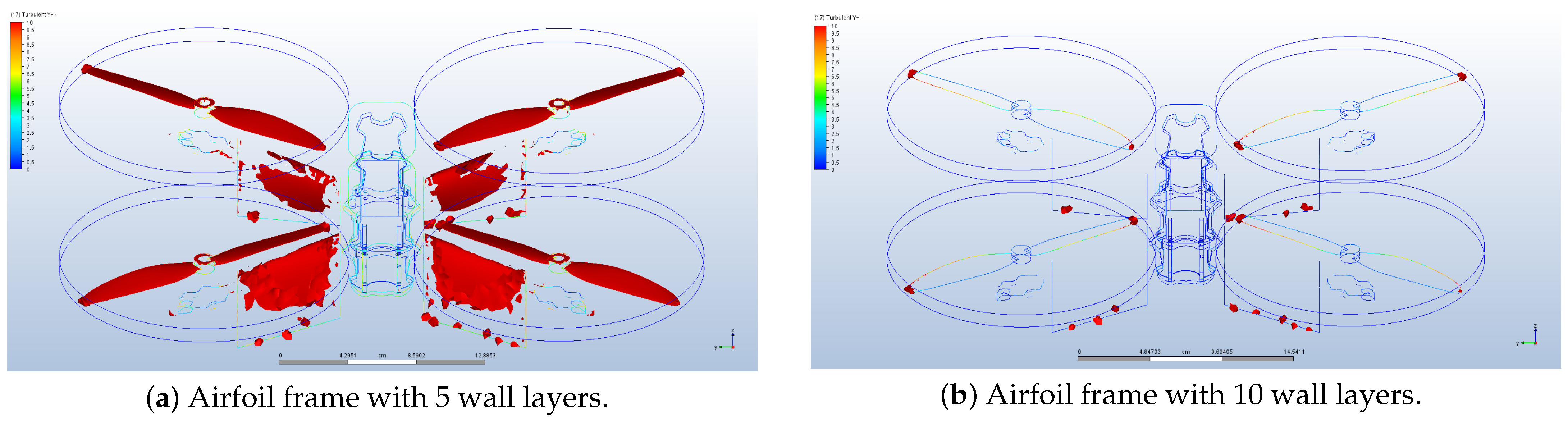
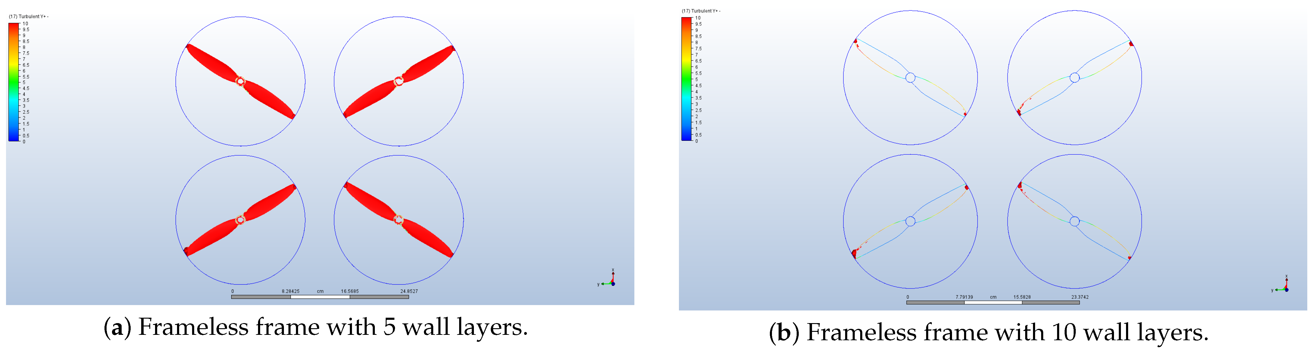
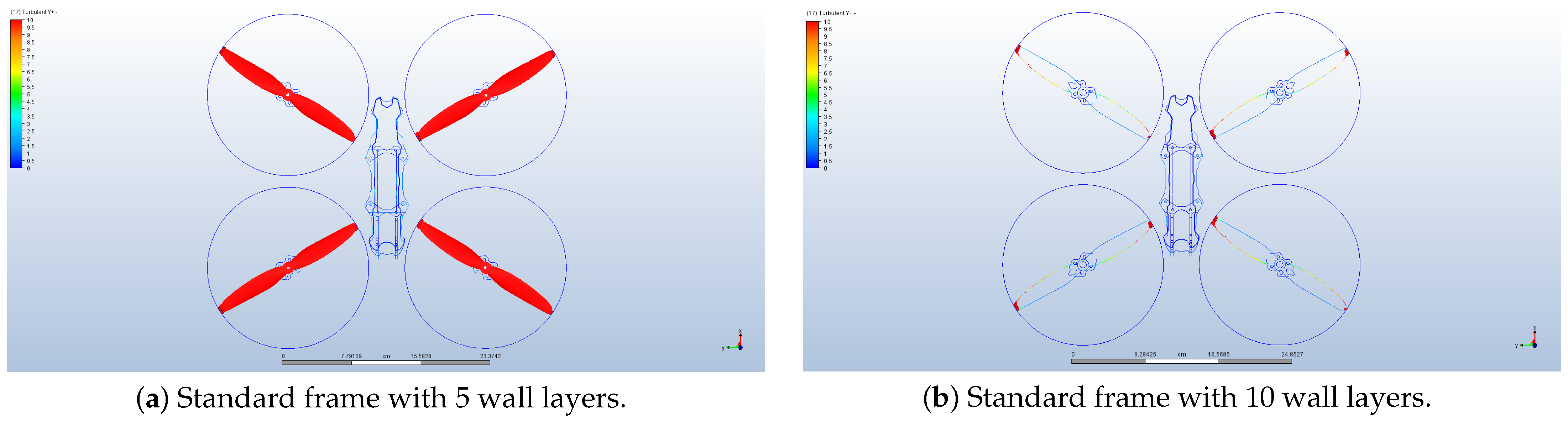
Appendix E. Turbulence Model Verification

According to Davidson and Salim [78], in CFD analysis, the term Y+ is a dimensionless quantity that measures the distance from a wall in relation to the viscous sublayer in turbulent flow near a boundary, such as the surface of a solid object. It is particularly important in turbulent flow simulations because it directly relates to the accuracy of how the simulation models the boundary layer. Essentially, it helps describe how fine or coarse the mesh is near the walls.
Getting the right Y+ is vital for accurate predictions of wall shear stress, heat transfer, and overall flow behavior, especially in turbulent cases. Ariff et al. [79] noted that different turbulence models in CFD often have specific requirements or guidelines for Y+ values at the wall to ensure the model functions correctly. Similarly, if a simulation uses “wall functions” to estimate flow behavior near walls, these functions have limitations on the acceptable range of Y+ values. The ideal range depends on factors like the turbulence model being used, whether wall functions are employed, and the specific goals of the simulation. Autodesk documentation on “Additional Mesh Adaptation Parameters” [80] notes that, according to the Turbulent Law of the Wall and numerous studies, the ideal range for Y+ is between 35 and 350, the default upper limit for Y+ Adaptation is 300, and, in some demanding cases such as very high-speed aerodynamics, it may be necessary to reduce the Max Y+ to achieve the desired accuracy.
CFD simulations often involve an iterative process where we run an initial simulation, check the resulting Y+ values, and then refine the mesh as needed to achieve the desired range.
Similarly to the mesh sensitivity study in Appendix D, only two meshes are required for each frame simulation: one for horizontal flight conditions and the other for leveled flight conditions. Thus, it is only necessary to perform the Y+ analysis twice for each frame and not for every single simulated flight condition.
According to Autodesk’s Rotating Region analysis best practices [81], which apply to multicopter aerodynamic simulations, it is suggested to use the SST K- ω turbulence model; thus, it is important to maintain a low value of Y+, although a value up to 10 can be satisfactory.
Autodesk’s “Wall Layers” documentation [82] explains that to decrease Y+ values when using the SST K- ω turbulence model, the number of wall layers can be increased from 5 (default) to 10 and, as a consequence, the layer gradation, which controls the rate of growth of the wall layers, should be changed from “Auto” to 1.5.
Upon examining Figure A2, Figure A3, Figure A4, Figure A5, Figure A6 and Figure A7, it is evident that most of the mesh elements with a Y+ value exceeding 10 (indicated by red zones) are situated at or near the propellers, which is expected due to their high rotational speed. Furthermore, it is clear that increasing the number of wall layers from 5 to 10 significantly reduces the extent of these red zones to just the tips of the propellers.
Figure A2. Y+ variation with wall layer increment for frameless frame performing horizontal flight.
Drones 09 00202 g0a2
Figure A3. Y+ variation with wall layer increment for standard frame performing horizontal flight.
Drones 09 00202 g0a3
Figure A4. Y+ variation with wall layer increment for airfoil frame performing horizontal flight.
Drones 09 00202 g0a4
Figure A5. Y+ variation with wall layer increment for frameless frame performing leveled flight.
Drones 09 00202 g0a5
Figure A6. Y+ variation with wall layer increment for standard frame performing leveled flight.
Drones 09 00202 g0a6
Figure A7. Y+ variation with wall layer increment for airfoil frame performing leveled flight.
Drones 09 00202 g0a7
It is evident from Table A6 and Table A7 that increasing the number of mesh walls from 5 to 10 leads to an average increase in the obtained aerodynamic forces of 6.4% to the horizontal flight mesh and 7.1% to the leveled flight mesh. This indicates that users aiming for a more accurate representation of the flow in each flight condition simulation can achieve some improvement in accuracy, albeit at the cost of increased computational time (as illustrated by the increased element count in Table A8 and Table A9).
Table A6. Results of wall number increment of horizontal flight mesh.
Horizontal Flight
ForceFrameWall LayersDifference
[%]
Average
per Axis [%]
Total
Average [%]
510
Fx [N]Frameless−5.779−6.2037.38.46.4
Standard Frame−4.223−4.5768.4
Airfoil Frame−3.818−4.1779.4
Fy [N]Frameless0.0030.036--
Standard Frame−0.084−0.033-
Airfoil Frame−0.092−0.049-
Fz [N]Frameless10.42010.8834.44.4
Standard Frame9.3899.9265.7
Airfoil Frame10.52310.8383.0
Table A7. Results of wall number increment of leveled flight mesh.
Leveled Flight
ForceFrameWall LayersDifference
[%]
Average
per Axis [%]
Total
Average [%]
510
Fx [N]Frameless0.0270.013--7.1
Standard Frame−0.0030.199-
Airfoil Frame−0.371−0.246-
Fy [N]Frameless0.0230.015--
Standard Frame0.0520.031-
Airfoil Frame0.1530.065-
Fz [N]Frameless14.37715.5808.47.1
Standard Frame12.55113.3986.7
Airfoil Frame13.24714.0546.1
Table A8. Element count for wall number increment of horizontal flight mesh.
Element Count (Horizontal Flight)
FrameWall LayersDifference [%]Average [%]
510
Frameless439,447496,22612.911.2
Standard Frame3,098,5883,434,24710.8
Airfoil Frame2,988,2143,282,8039.9
Table A9. Element count for wall number increment of leveled flight mesh.
Element Count (Leveled Flight)
FrameWall LayersDifference [%]Average [%]
510
Frameless430,154492,19314.412.5
Standard Frame2,809,9633,144,66211.9
Airfoil Frame2,622,6672,915,42911.2
In this context, the most significant result is the difference in the forces obtained with standard and airfoil frames compared to the frameless case, which allows us to determine the lift and drag induced by each frame. Notably, after increasing the number of wall layers, the force results for all frames rise by approximately the same percentage for each axis (maximum difference of 2.7%). Therefore, the differences in lift and drag between each frame will also increase by roughly the same percentage, which ultimately does not alter the conclusions of this study.

References

  1. Hardin, P.J.; Hardin, T.J. Small-scale remotely piloted vehicles in environmental research. Geogr. Compass 2010, 4, 1297–1311. [Google Scholar] [CrossRef]
  2. Young, L.; Yetter, J.; Guynn, M. System analysis applied to autonomy: Application to high-altitude long-endurance remotely operated aircraft. In Proceedings of the Infotech@ Aerospace, Arlington, VA, USA, 26–29 September 2005; p. 7103. [Google Scholar]
  3. Chabot, D. Trends in drone research and applications as the Journal of Unmanned Vehicle Systems turns five. J. Unmanned Veh. Syst. 2018, 6, vi–xv. [Google Scholar] [CrossRef]
  4. Hassanalian, M.; Abdelkefi, A. Classifications, applications, and design challenges of drones: A review. Prog. Aerosp. Sci. 2017, 91, 99–131. [Google Scholar] [CrossRef]
  5. Nahiyoon, S.A.; Ren, Z.; Wei, P.; Li, X.; Li, X.; Xu, J.; Yan, X.; Yuan, H. Recent Development Trends in Plant Protection UAVs: A Journey from Conventional Practices to Cutting-Edge Technologies—A Comprehensive Review. Drones 2024, 8, 457. [Google Scholar] [CrossRef]
  6. Frachtenberg, E. Practical drone delivery. Computer 2019, 52, 53–57. [Google Scholar] [CrossRef]
  7. Viana, J.; Cercas, F.; Correia, A.; Dinis, R.; Sebastião, P. MIMO Relaying UAVs Operating in Public Safety Scenarios. Drones 2021, 5, 32. [Google Scholar] [CrossRef]
  8. Álvarez González, M.; Suarez-Bregua, P.; Pierce, G.J.; Saavedra, C. Unmanned Aerial Vehicles (UAVs) in Marine Mammal Research: A Review of Current Applications and Challenges. Drones 2023, 7, 667. [Google Scholar] [CrossRef]
  9. Munawar, H.S.; Ullah, F.; Heravi, A.; Thaheem, M.J.; Maqsoom, A. Inspecting Buildings Using Drones and Computer Vision: A Machine Learning Approach to Detect Cracks and Damages. Drones 2022, 6, 5. [Google Scholar] [CrossRef]
  10. Pan, L.; Song, C.; Gan, X.; Xu, K.; Xie, Y. Military Image Captioning for Low-Altitude UAV or UGV Perspectives. Drones 2024, 8, 421. [Google Scholar] [CrossRef]
  11. Rennie, J. Drone Types: Multi-Rotor vs. Fixed-Wing vs. Single Rotor vs. Hybrid Vtol. AUAV Com 2016, 19, 2024. [Google Scholar]
  12. Ducard, G.J.; Allenspach, M. Review of designs and flight control techniques of hybrid and convertible VTOL UAVs. Aerosp. Sci. Technol. 2021, 118, 107035. [Google Scholar] [CrossRef]
  13. Kunertova, D. The war in Ukraine shows the game-changing effect of drones depends on the game. Bull. At. Sci. 2023, 79, 95–102. [Google Scholar] [CrossRef]
  14. Seo, K.I.; Cho, S.K.; Park, S.H. A Case Study on FPV Drone Combats of the Ukrainian Forces. J. Converg. Cult. Technol. 2023, 9, 263–270. [Google Scholar]
  15. Stewart, M.; Martin, S.; Barrera, N. Unmanned aerial vehicles: Fundamentals, components, mechanics, and regulations. Unmanned Aer. Veh. 2021, 3, 1–70. [Google Scholar]
  16. Liu, R.l.; Zhang, Z.j.; Jiao, Y.f.; Yang, C.h.; Zhang, W.j. Study on Flight Performance of Propeller-Driven UAV. Int. J. Aerosp. Eng. 2019, 2019, 6282451. [Google Scholar] [CrossRef]
  17. Biczyski, M.; Sehab, R.; Whidborne, J.F.; Krebs, G.; Luk, P. Multirotor sizing methodology with flight time estimation. J. Adv. Transp. 2020, 2020, 9689604. [Google Scholar] [CrossRef]
  18. Nagel, L. How Does Drone Payload Affect Flight Time. 2024. Available online: https://www.tytorobotics.com/blogs/articles/how-does-drone-payload-affect-flight-time (accessed on 12 September 2024).
  19. Kumar, V.A.; Sivaguru, M.; Janaki, B.R.; Eswar, K.S.; Kiran, P.; Vijayanandh, R. Structural optimization of frame of the multi-rotor unmanned aerial vehicle through computational structural analysis. In Proceedings of the Journal of Physics: Conference Series, Volume 1849, 2nd National Conference on Recent Advancement in Physical Sciences, (NCRAPS) 2020, Uttarakhand, India, 19–20 December 2020; Volume 1849, p. 012004. [Google Scholar]
  20. Müller, M. eCalc: The Most Reliable RC Calculator on the Web. Online Resource. 2014. Available online: https://www.ecalc.ch (accessed on 12 February 2025).
  21. Eppler, R. Airfoil Design and Data; Springer Science & Business Media: Berlin/Heidelberg, Germany, 2012. [Google Scholar]
  22. Jha, D.; Singh, M.; Thakur, A. A novel computational approach for design and performance investigation of small wind turbine blade with extended BEM theory. Int. J. Energy Environ. Eng. 2021, 12, 563–575. [Google Scholar] [CrossRef]
  23. AirShaper. Fundamentals of Airfoil Design and Selection. Available online: https://airshaper.com/videos/airfoil-design-for-a-drone/kAXN3MlQxxc (accessed on 11 September 2024).
  24. Anderson, J. A History of Aerodynamics: And Its Impact on Flying Machines; Cambridge Aerospace Series; Cambridge University Press: Cambridge, UK, 1998. [Google Scholar]
  25. LaNasa, P.J.; Upp, E.L. 2—Basic Flow Measurement Laws. In Fluid Flow Measurement, 3rd ed.; LaNasa, P.J., Upp, E.L., Eds.; Butterworth-Heinemann: Oxford, UK, 2014; pp. 19–29. [Google Scholar] [CrossRef]
  26. Haryanto, I.; Utomo, T.S.; Sinaga, N.; Rosalia, C.A.; Putra, A.P. Optimization of maximum lift to drag ratio on airfoil design based on artificial neural network utilizing genetic algorithm. Appl. Mech. Mater. 2014, 493, 123–128. [Google Scholar] [CrossRef]
  27. HopsonRoad. Coefficient of Lift (CL) and Coefficient of Drag (CD) and Their Ratio as a Function of Angle of Attack for a Hypothetical Sail. The Status of Flow Between Attached to Separated is Shown in Relation to the Curve. Available online: https://commons.wikimedia.org/wiki/File:Coefficients_of_Lift_and_Drag_for_a_Hypothetical_Sail.png#file (accessed on 12 February 2025).
  28. Kay, N.J.; Richards, P.J.; Sharma, R.N. Influence of turbulence on cambered and symmetrical airfoils at low Reynolds numbers. AIAA J. 2020, 58, 1913–1925. [Google Scholar] [CrossRef]
  29. Merzkirch, W. Flow Visualization; Elsevier: Amsterdam, The Netherlands, 2012. [Google Scholar]
  30. Chang, P.K. Separation of Flow; Elsevier: Amsterdam, The Netherlands, 2014. [Google Scholar]
  31. Prandtl, L.; Oswatitsch, K.; Wieghardt, K. Flugkörper, Antriebe und Strömungsmaschinen. In Führer Durch die Strömungslehre; Vieweg+Teubner Verlag: Wiesbaden, Germany, 1990; pp. 430–524. [Google Scholar] [CrossRef]
  32. Abbott, I.H.; Von Doenhoff, A.E.; Stivers, L., Jr. Summary of Airfoil Data. Technical Report, National Advisory Committee for Aeronautics (NACA), 1945. Report No.: NACA Report No. 824. Available online: https://ntrs.nasa.gov/citations/19930090976 (accessed on 12 February 2025).
  33. Anderson, J.D.; Wendt, J. Computational Fluid Dynamics; Springer: Berlin/Heidelberg, Germany, 1995; Volume 206. [Google Scholar]
  34. Kopal, Z. Tables of Supersonic Flow Around Cones; Number 1; Massachusetts Institute of Technology: Cambridge, MA, USA, 1947. [Google Scholar]
  35. Moretti, G.; Abbett, M. A time-dependent computational method for blunt body flows. AIAA J. 1966, 4, 2136–2141. [Google Scholar] [CrossRef]
  36. Team, A. Autodesk CFD: Simulation Software for Engineering Complex Liquid, Gas, and Air Systems. Version 2024. Available online: https://www.autodesk.com/eu/products/cfd/overview (accessed on 13 November 2024).
  37. Zhai, Z.J.; Zhang, Z.; Zhang, W.; Chen, Q.Y. Evaluation of various turbulence models in predicting airflow and turbulence in enclosed environments by CFD: Part 1—Summary of prevalent turbulence models. Hvac&R Res. 2007, 13, 853–870. [Google Scholar]
  38. GEPRC. GEP-Mark4-7 Frame. Available online: https://geprc.com/product/gep-mark4-7-frame/ (accessed on 20 December 2024).
  39. Gemfan. Gemfan LR 7035-2 for Long Range. Available online: https://www.gfprops.com/product/index/details/id/10785.html (accessed on 20 December 2024).
  40. T-Motor. F90 2806.5 Long Range Motor 5-6S KV1300. Available online: https://shop.tmotor.com/products/brushless-motor-x8-fpv-drones-f90-2806-5?srsltid=AfmBOoox2djP41i6SgBQwhez03oQTZr8chCSSo_n31AIIdTqwLZFLMUg (accessed on 10 March 2025).
  41. Holybro. Tekko32 F4 Metal 4in1 65A ESC. Available online: https://holybro.com/products/tekko32-f4-metal-4in1-65a-esc-65a (accessed on 20 December 2024).
  42. Samsung. Samsung INR21700-50S 5000mAh—35A. Available online: https://www.nkon.nl/pt/rechargeable/li-ion/21700-20700-size/samsung-inr21700-50s-5000mah-35a.html (accessed on 20 December 2024).
  43. Team, A. Autodesk Fusion: More Than CAD, It’s the Future of Design and Manufacturing. Version 2024. Available online: https://www.autodesk.com/eu/products/fusion-360/overview?term=1-YEAR&tab=subscription (accessed on 13 November 2024).
  44. Hwang, M.h.; Cha, H.R.; Jung, S.Y. Practical Endurance Estimation for Minimizing Energy Consumption of Multirotor Unmanned Aerial Vehicles. Energies 2018, 11, 2221. [Google Scholar] [CrossRef]
  45. Tools, A. Airfoil Tools. Available online: http://airfoiltools.com/ (accessed on 12 November 2024).
  46. Community, A. Connect ESCs and Motors. Available online: https://ardupilot.org/copter/docs/connect-escs-and-motors.html (accessed on 13 September 2024).
  47. Prusa, J. Prusa Slicer. Available online: https://www.prusa3d.com/page/prusaslicer_424/ (accessed on 19 November 2024).
  48. Bulota, M.; Budtova, T. Highly porous and light-weight flax/PLA composites. Ind. Crop. Prod. 2015, 74, 132–138. [Google Scholar] [CrossRef]
  49. Standau, T.; Zhao, C.; Murillo Castellón, S.; Bonten, C.; Altstädt, V. Chemical modification and foam processing of polylactide (PLA). Polymers 2019, 11, 306. [Google Scholar] [CrossRef]
  50. Xiao, K.; Meng, Y.; Dai, X.; Zhang, H.; Quan, Q. A lifting wing fixed on multirotor UAVs for long flight ranges. In Proceedings of the 2021 International Conference on Unmanned Aircraft Systems (ICUAS), Athens, Greece, 15–18 June 2021; pp. 1605–1610. [Google Scholar]
  51. Autodesk CFD 2024. Centrifugal Pumps and Axial Fans. Available online: https://help.autodesk.com/view/SCDSE/2024/ENU/?guid=GUID-013A783C-807F-4340-BB8B-16A3AF52EECA (accessed on 13 November 2024).
  52. Autodesk CFD 2024. Turbulence. Available online: https://help.autodesk.com/view/SCDSE/2024/ENU/?guid=GUID-E9E8ACA1-8D49-4A49-8A35-52DB1A2C3E5F (accessed on 13 November 2024).
  53. Help, A. Compressible Flow. Available online: https://help.autodesk.com/view/SCDSE/2024/ENU/?guid=GUID-620F44CE-9506-4C48-9E9C-6C689345B008 (accessed on 13 September 2024).
  54. Help, A. Advection Schemes. Available online: https://help.autodesk.com/view/SCDSE/2024/ENU/?guid=GUID-F691B334-CCE2-47E9-B6C4-21666712C163 (accessed on 13 September 2024).
  55. Liang, O. Types of Multirotor. 2016. Available online: https://oscarliang.com/types-of-multicopter/ (accessed on 11 September 2024).
  56. Achtelik, M.; Doth, K.M.; Gurdan, D.; Stumpf, J. Design of a multi rotor MAV with regard to efficiency, dynamics and redundancy. In Proceedings of the AIAA Guidance, Navigation, and Control Conference, Minneapolis, MN, USA, 13–16 August 2012; p. 4779. [Google Scholar]
  57. Toglefritz, L. Types of Multirotor. Available online: https://toglefritz.com/types-of-multirotor/ (accessed on 18 November 2024).
  58. Bondyra, A.; Gardecki, S.; Gasior, P.; Giernacki, W. Performance of coaxial propulsion in design of multi-rotor UAVs. In Proceedings of the Challenges in Automation, Robotics and Measurement Techniques: Proceedings of AUTOMATION-2016, Warsaw, Poland, 2–4 March 2016; Springer: Berlin/Heidelberg, Germany, 2016; pp. 523–531. [Google Scholar]
  59. Theys, B.; Dimitriadis, G.; Hendrick, P.; De Schutter, J. Influence of propeller configuration on propulsion system efficiency of multi-rotor Unmanned Aerial Vehicles. In Proceedings of the 2016 International Conference on Unmanned Aircraft Systems (ICUAS), Arlington, VA, USA, 7–10 June 2016; pp. 195–201. [Google Scholar]
  60. Liang, O. The Ultimate Guide to FPV Drone Propellers: How to Choose the Best Props for Your Quadcopter. 2024. Available online: https://oscarliang.com/propellers/ (accessed on 11 September 2024).
  61. Kovtun, A. Influence of the shape and number of blades on the efficiency of the UAV propeller. Aerosp. Tech. Technol. 2024, 31–37. [Google Scholar] [CrossRef]
  62. Podsędkowski, M.; Konopiński, R.; Obidowski, D.; Koter, K. Variable Pitch Propeller for UAV-Experimental Tests. Energies 2020, 13, 5264. [Google Scholar] [CrossRef]
  63. Ramesh, M.; Vijayanandh, R.; Kumar, G.R.; Mathaiyan, V.; Jagadeeshwaran, P.; Kumar, M.S. Comparative structural analysis of various composite materials based unmanned aerial vehicle’s propeller by using advanced methodologies. In Proceedings of the IOP Conference Series: Materials Science and Engineering, Jaipur, India, 5–6 November 2020; IOP Publishing: Bristol, UK, 2021; Volume 1017, p. 012032. [Google Scholar]
  64. Putra, H.; Fikri, M.; Riananda, D.; Nugraha, G.; Baidhowi, M.; Syah, R. Propulsion selection method using motor thrust table for optimum flight in multirotor aircraft. AIP Conf. Proc. 2020, 2226, 060008. [Google Scholar]
  65. Uçar, U.U.; Adem, A.; Tanyeri, B. A Multi-Criteria Solution Approach for UAV Engine Selection in Terms of Technical Specification. Bitlis Eren Üniversitesi Fen Bilim. Derg. 2022, 11, 1000–1013. [Google Scholar] [CrossRef]
  66. Bershadsky, D.; Haviland, S.; Johnson, E.N. Electric multirotor UAV propulsion system sizing for performance prediction and design optimization. In Proceedings of the 57th AIAA/ASCE/AHS/ASC Structures, Structural Dynamics, and Materials Conference, San Diego, CA, USA, 4–8 January 2016; p. 0581. [Google Scholar]
  67. Liang, O. Understanding ESCs for FPV Drones: How to Choose the Best Electronic Speed Controller. 2024. Available online: https://oscarliang.com/esc/ (accessed on 11 September 2024).
  68. Delbecq, S.; Budinger, M.; Ochotorena, A.; Reysset, A.; Defaÿ, F. Efficient sizing and optimization of multirotor drones based on scaling laws and similarity models. Aerosp. Sci. Technol. 2020, 102, 105873. [Google Scholar] [CrossRef]
  69. Liang, O. Using LiPo Batteries for FPV Drones: Beginner’s Guide with Top Product Recommendations. 2024. Available online: https://oscarliang.com/lipo-battery-guide/ (accessed on 20 December 2024).
  70. Leishman, J.G. Introduction to Aerospace Flight Vehicles; Embry-Riddle Aeronautical University: Daytona Beach, FL, USA, 2023. [Google Scholar]
  71. Scott, J. NACA Airfoil Series. Available online: https://aerospaceweb.org/question/airfoils/q0041.shtml (accessed on 19 November 2024).
  72. Mohamed, O.A.; Masood, S.H.; Bhowmik, J.L. Optimization of fused deposition modeling process parameters: A review of current research and future prospects. Adv. Manuf. 2015, 3, 42–53. [Google Scholar] [CrossRef]
  73. Chennakesava, P.; Narayan, Y.S. Fused deposition modeling-insights. In Proceedings of the International Conference on Advances in Design and Manufacturing ICAD&M, Tiruchirappalli, Tamil Nadu, India, 5–7 December 2014; Volume 14, p. 1345. [Google Scholar]
  74. Rajan, K.; Samykano, M.; Kadirgama, K.; Harun, W.S.W.; Rahman, M.M. Fused deposition modeling: Process, materials, parameters, properties, and applications. Int. J. Adv. Manuf. Technol. 2022, 120, 1531–1570. [Google Scholar] [CrossRef]
  75. Zhao, H.; Liu, X.; Zhao, W.; Wang, G.; Liu, B. An overview of research on FDM 3D printing process of continuous fiber reinforced composites. J. Phys. Conf. Ser. 2019, 1213, 052037. [Google Scholar] [CrossRef]
  76. Oktay, T.; Eraslan, Y. Mesh Independence Study on Computational Fluid Dynamics (CFD) Analysis of a Quad-rotor UAV Propeller. In Proceedings of the 3rd International European Conference on Interdisciplinary Scientific Researches, Comrat, Moldova, 15–16 January 2021. [Google Scholar]
  77. Support, A. How to Manually Perform a Mesh Sensitivity Study in Simulation CFD. Available online: https://www.autodesk.com/support/technical/article/caas/sfdcarticles/sfdcarticles/How-to-manually-perform-a-mesh-sensitivity-study-in-Simulation-CFD.html (accessed on 11 February 2025).
  78. Davidson, A.A.; Salim, S.M. Wall y+ strategy for modelling rotating annular flow using CFD. In Proceedings of the 2018 International MultiConference of Engineers and Computer Scientists, IMECS 2018, Hong Kong, China, 14–16 March 2018; Newswood Limited: Hong Kong, China, 2018. [Google Scholar]
  79. Ariff, M.; Salim, S.M.; Cheah, S.C. Wall y+ approach for dealing with turbulent flow over a surface mounted cube: Part 1—low Reynolds number. In Proceedings of the Seventh International Conference on CFD in the Minerals and Process Industries, Melbourne, Australia, 9–11 December 2009; CSIRO Publishing Melbourne: Melbourne, Australia, 2009; pp. 1–6. [Google Scholar]
  80. Autodesk CFD 2024. Additional Mesh Adaptation Parameters. Available online: https://help.autodesk.com/view/SCDSE/2024/ENU/?guid=GUID-D074870E-E00C-460C-B611-42B3FABCE418 (accessed on 17 February 2025).
  81. Support, A. Best Practices for Running a Rotating Region Analysis in Autodesk CFD. Available online: https://www.autodesk.com/support/technical/article/caas/sfdcarticles/sfdcarticles/What-are-the-best-practices-for-running-a-rotating-region-analysis-in-Simulation-CFD.html (accessed on 14 February 2025).
  82. Autodesk CFD 2024. Wall Layers. Available online: https://help.autodesk.com/view/SCDSE/2024/ENU/?guid=GUID-F9C4DDB4-8111-4F25-8EDE-D7C38B3BAD99 (accessed on 17 February 2025).
Figure 1. Airfoil parameter nomenclature provided by Jha et al. [22].
Drones 09 00202 g001
Figure 4. Simplified model of standard frame UAV.
Drones 09 00202 g004
Figure 5. UAV performance estimates by eCalc.
Drones 09 00202 g005
Figure 6. Flow simulation visualization of a standard frame UAV at the root of the arms cross-section for flight conditions of 20 m/s external airflow speed and propellers rotating at 20,000 RPMs.
Drones 09 00202 g006
Figure 7. Flow simulation visualization of a standard frame UAV at the tip of the arms cross-section for flight conditions of 20 m/s external airflow speed and propellers rotating at 20,000 RPMs.
Drones 09 00202 g007
Figure 8. The schematics of a planar view for a forward flight drone. An adapted illustration from Hwang et al. [44].
Drones 09 00202 g008
Figure 9. NACA 0030 airfoil.
Drones 09 00202 g009
Figure 10. An airfoil sketch at the root of the frame arms.
Drones 09 00202 g010
Figure 11. An airfoil sketch at the tip of the frame arms.
Drones 09 00202 g011
Figure 12. Simplified model of airfoil frame UAV.
Drones 09 00202 g012
Figure 13. Propellers-in vs. propellers-out configuration. Adapted illustration from Ardupilot Community [46].
Drones 09 00202 g013
Figure 14. Flow simulation visualization of a standard frame UAV (propellers-in configuration) at the root of the arms cross-section for flight conditions of 20 m/s external airflow speed and propellers rotating at 20,000 RPMs.
Drones 09 00202 g014
Figure 15. Flow simulation visualization of a standard frame UAV (propellers-in configuration) at the tip of the arms cross-section for flight conditions of 20 m/s external airflow speed and propellers rotating at 20,000 RPMs.
Drones 09 00202 g015
Figure 16. Convergence Monitor of one of the performed analyses.
Drones 09 00202 g016
Figure 17. Flow simulation visualization at time step 2000 (converged analysis) for frameless UAV at plane y = 5 (“arm” cross-section) for flight conditions of 20 m/s external airflow speed and propellers rotating at 20,000 RPMs.
Drones 09 00202 g017
Figure 18. Flow simulation visualization at time step 2000 (converged analysis) of standard frame UAV at plane y = 5 (arm cross-section) for flight conditions of 20 m/s external airflow speed and propellers rotating at 20,000 RPMs.
Drones 09 00202 g018
Figure 19. Flow simulation visualization at time step 2000 (converged analysis) of airfoil frame UAV at plane y = 5 (arm cross-section) for flight conditions of 20 m/s external airflow speed and propellers rotating at 20,000 RPMs.
Drones 09 00202 g019
Table 1. Unmanned Aerial Vehicle component list.
ComponentReasons for Selection
FrameGEPRC MK4 7 inch [38]Common quadrotor configuration;
Simplicity;
Lightness;
Carbon fiber (impact-resistant);
Affordable;
Largest size acceptable for this mission;
PropellerGemfan LR 7035 2-Blades [39]Maximum diameter for the selected frame;
Low pitch;
High efficiency;
Two blades;
MotorT-Motor F90 1300 KV [40]Adequate size for required torque;
Low KV for higher efficiency;
ESCHolybro Tekko32 F4
Metal 4in1 65A ESC [41]
Metal-cased mosfets for improved heat dissipation;
Large maximum current rating;
Four-in-one configuration (less complexity and lighter);
BatterySamsung INR21700-50S
5000 mAh—35A (4S Pack) [42]
Li-ion chemistry (high energy density);
Highest capacity and continuous discharge current Li-ion cell available at this time.
Table 2. Results of simulations conducted at horizontal flight, with varying external flow speed and fixed propeller RPMs.
F X [N] F Y [N] F Z [N] F D [N] C D F L [N]AAW [g]
15 m/s External Flow Speed at 20,000 rpm
Frameless−6.263−0.02611.081----
Standard Frame−5.126−0.03610.361.1370.676−0.72173.5
Airfoil Frame−5.147−0.09111.3611.1160.3870.280−28.6
20 m/s External Flow Speed at 20,000 rpm
Frameless−5.7790.00310.420----
Standard Frame−4.223−0.0849.3891.5560.520−1.031105.1
Airfoil Frame−3.818−0.09210.5231.9610.3830.103−10.5
25 m/s External Flow Speed at 20,000 rpm
Frameless−5.0800.0029.231----
Standard Frame−2.9250.0198.0642.1550.461−1.167119.0
Airfoil Frame−2.044−0.0319.4003.0360.3790.169−17.2
Table 3. Results of simulations conducted at horizontal flight, with fixed external flow and varying propeller RPMs.
F X [N] F Y [N] F Z [N] F D [N] C D F L [N]AAW [g]
20 m/s External Flow Speed at 15,000 rpm
Frameless−2.715−0.0014.939----
Standard Frame−1.3660.0344.2471.3490.451−0.69270.6
Airfoil Frame−0.779−0.0345.0661.9360.3780.127−12.9
20 m/s External Flow Speed at 20,000 rpm
Frameless−5.7790.00310.420----
Standard Frame−4.223−0.0849.3891.5560.520−1.031105.1
Airfoil Frame−3.818−0.09210.5231.9610.3830.103−10.5
20 m/s External Flow Speed at 25,000 rpm
Frameless−9.6880.00817.411----
Standard Frame−7.780−0.02415.9061.9080.638−1.505153.5
Airfoil Frame−7.670−0.15217.5392.0180.3940.128-13.1
Table 4. Results from the simulations conducted at leveled flight, with varying external flow and fixed propeller RPMs.
F X [N] F Y [N] F Z [N] F D [N] C D F L [N]AAW [g]
5 m/s Descending Flow at 20,000 rpm
Frameless0.010−0.00914.181----
Standard Frame0.0000.01112.080--−2.101214.2
Airfoil Frame−0.3630.08612.852--−1.329135.5
Steady External Flow at 20,000 rpm
Frameless0.0270.02314.377----
Standard Frame−0.0030.05212.551--−1.826186.2
Airfoil Frame−0.3710.15313.247--−1.130115.2
5 m/s Ascending Flow at 20,000 rpm
Frameless0.0160.00914.183----
Standard Frame−0.026−0.11312.941--−1.242126.6
Airfoil Frame−0.2790.13313.898--−0.28529.1
Table 5. Results from simulations conducted at leveled flight, with steady external flow and varying propeller RPMs.
F X [N] F Y [N] F Z [N] F D [N] C D F L [N]AAW [g]
Steady External Flow at 15,000 rpm
Frameless0.005−0.0108.308----
Standard Frame−0.0020.0327.085--−1.223124.7
Airfoil Frame−0.1650.0427.473--−0.83585.1
Steady External Flow at 20,000 rpm
Frameless0.0270.02314.377----
Standard Frame−0.0030.05212.551--−1.826186.2
Airfoil Frame−0.3710.15313.247--−1.130115.2
Steady External Flow at 25,000 rpm
Frameless0.014−0.01323.054----
Standard Frame−0.0030.12019.657--−3.397346.4
Airfoil Frame−0.3460.28420.776--−2.278232.3
Table 6. Lift comparison between the standard and airfoil frames during horizontal flight conditions.
Lift
Flight ConditionStandard Frame [N]Airfoil Frame [N]Comparison [%]
15 m/s at 20,000 rpm−0.7210.280138.8
20 m/s at 20,000 rpm−1.0310.103110.0
25 m/s at 20,000 rpm−1.1670.169114.5
20 m/s at 15,000 rpm−0.6920.127118.4
20 m/s at 25,000 rpm−1.5050.128108.5
Average−1.0230.161118.0
Table 7. AAW comparison between standard and airfoil frames during horizontal flight conditions.
Aerodynamic Added Weight (AAW)
Flight ConditionStandard Frame [g]Airfoil Frame [g]Comparison [%]
15 m/s at 20,000 rpm73.5−28.6−138.8
20 m/s at 20,000 rpm105.1−10.5−110.0
25 m/s at 20,000 rpm119.0−17.2−114.5
20 m/s at 15,000 rpm70.6−12.9−118.4
20 m/s at 25,000 rpm153.5−13.1−108.5
Average104.3−16.5−118.0
Table 8. Momentary weight comparison between the standard and airfoil frames during horizontal flight conditions.
Momentary Weight
Flight ConditionStandard Frame (Frame + AAW) [g]Airfoil Frame (Frame + Airfoils + AAW) [g]Comparison [%]
15 m/s at 20,000 rpm10741019−5.0
20 m/s at 20,000 rpm11051037−6.1
25 m/s at 20,000 rpm11191031−7.9
20 m/s at 15,000 rpm10711035−3.3
20 m/s at 25,000 rpm11531035−10.3
Average11041032−6.5
Table 9. Mixed flight time estimate comparison between standard and airfoil frames during horizontal flight conditions.
Flight Time Estimate from eCalc (Mixed Flight Time)
Flight ConditionStandard Frame [min]Airfoil Frame [min]Comparison [%]
15 m/s at 20,000 rpm12.012.75.8
20 m/s at 20,000 rpm11.712.56.8
25 m/s at 20,000 rpm11.512.69.6
20 m/s at 15,000 rpm12.112.53.3
20 m/s at 25,000 rpm11.112.512.6
Average11.712.67.6
Table 10. Drag comparison between standard and airfoil frames during horizontal flight conditions.
Drag
Flight ConditionStandard Frame [N]Airfoil Frame [N]Comparison [%]
15 m/s at 20,000 rpm1.1371.116−1.8
20 m/s at 20 000 rpm1.5561.96126.0
25 m/s at 20,000 rpm2.1553.03640.9
20 m/s at 15,000 rpm1.3491.93643.5
20 m/s at 25,000 rpm1.9082.0185.8
Average1.6212.01322.9
Table 11. Drag coefficient ( C D ) comparison between standard and airfoil frames during horizontal flight conditions.
Drag Coefficient ( C D )
Flight ConditionStandard FrameAirfoil FrameComparison [%]
15 m/s at 20,000 rpm0.6760.387−42.7
20 m/s at 20,000 rpm0.5200.383−26.4
25 m/s at 20,000 rpm0.4610.379−17.8
20 m/s at 15,000 rpm0.4510.378−16.2
20 m/s at 25,000 rpm0.6380.394−38.3
Average0.5490.384−28.3
Table 12. Lift comparison between standard and airfoil frames during leveled flight conditions.
Lift
Flight ConditionStandard Frame [N]Airfoil Frame [N]Comparison [%]
15,000 rpm−1.223−0.83531.7
20,000 rpm−1.826−1.13038.1
25,000 rpm−3.397−2.27832.9
−5 m/s at 20,000 rpm−2.101−1.32936.7
+5 m/s at 20,000 rpm−1.242−0.28577.1
Average−1.958−1.17143.3
Table 13. AAW comparison between standard and airfoil frames during leveled flight conditions.
Aerodynamic Added Weight (AAW)
Flight ConditionStandard Frame [g]Airfoil Frame [g]Comparison [%]
15,000 rpm124.785.1−31.7
20,000 rpm186.2115.2−38.1
25,000 rpm346.4232.3−32.9
−5 m/s at 20,000 rpm214.2135.5−36.7
+5 m/s at 20,000 rpm126.629.1−77.1
Average199.6119.4−43.3
Table 14. Momentary weight comparison between the standard and airfoil frames during leveled flight conditions.
Momentary Weight
Flight ConditionStandard Frame (Frame + AAW) [g]Airfoil Frame (Frame + Airfoils + AAW) [g]Comparison [%]
15,000 rpm112511330.8
20,000 rpm11861163−1.9
25,000 rpm13461280−4.9
−5 m/s at 20,000 rpm12141184−2.5
+5 m/s at 20,000 rpm11271077−4.4
Average12001167−2.6
Table 15. Hovering flight time estimate comparison between standard and airfoil frames.
Flight Time Estimate from eCalc (Hovering Flight Time)
Flight ConditionStandard Frame [min]Airfoil Frame [min]Comparison [%]
15,000 rpm14.714.5−1.4
20,000 rpm13.514.03.7
25,000 rpm11.012.09.1
−5 m/s at 20,000 rpm13.013.64.6
+5 m/s at 20,000 rpm14.715.76.8
Average13.414.04.6
Table 16. Longitudinal force comparison between standard and airfoil frames during leveled flight conditions.
Longitudinal Force
Flight ConditionStandard Frame [N]Airfoil Frame [N]
15,000 rpm−0.007−0.170
20,000 rpm−0.030−0.398
25,000 rpm−0.017−0.360
−5 m/s at 20,000 rpm−0.010−0.373
+5 m/s at 20,000 rpm−0.042−0.295
Average−0.021−0.319
Table 17. Transversal force comparison between standard and airfoil frames during leveled flight conditions.
Transversal Force
Flight ConditionStandard Frame [N]Airfoil Frame [N]
15,000 rpm0.0420.052
20,000 rpm0.0290.130
25,000 rpm0.1330.297
−5 m/s at 20,000 rpm0.0200.095
+5 m/s at 20,000 rpm−0.1220.124
Average0.0200.140
Disclaimer/Publisher’s Note: The statements, opinions and data contained in all publications are solely those of the individual author(s) and contributor(s) and not of MDPI and/or the editor(s). MDPI and/or the editor(s) disclaim responsibility for any injury to people or property resulting from any ideas, methods, instructions or products referred to in the content.

