An Anti-Disturbance Attitude Control Method for Fixed-Wing Unmanned Aerial Vehicles Based on an Integral Sliding Mode Under Complex Disturbances During Sea Flight

Abstract

The increasing complexity of aerial acrobatics missions necessitates ever-higher levels of attitude control precision in fixed-wing unmanned aerial vehicles (UAVs). Traditional control methods, such as feedback linearization and small disturbance derivation linear models, falter in maintaining attitude tracking accuracy, due to the presence of unanticipated disturbances—most notably, wave disturbances during low-altitude maritime flights—and model uncertainties introduced by factors like large-angle maneuvers, intricate aerodynamic characteristics, and fuel consumption. Consequently, these limitations impede the successful execution of intricate maneuvers, such as looping, the split-S, the Immelmann turn, and the Pougatcheff cobra maneuver. In response to these challenges, we propose an integral sliding mode control based on disturbance observer (ISMC-DO) system to achieve robust attitude angle tracking amidst model uncertainties and mitigate the effects of wave disturbances. Additionally, quaternion representations are adopted as a supplement to Euler angles, thereby resolving the singularity issues inherent in the latter. By using the Lyapunov function, the ISMC-DO-based control system is shown to be asymptotically stable. Simulation results further validate that ISMC-DO can achieve high-precision attitude tracking control of the UAV under wave disturbance.

1. Introduction

In recent years, fixed-wing unmanned aerial vehicles (UAVs) have garnered significant attention due to their notable advantages: rapid movement speed, extended flight range, expansive cruising areas, and elevated flight altitudes [1]. Owing to advances in intelligent flight control technology, the applications of fixed-wing UAVs have expanded considerably—ranging from air combat and aerial acrobatics to material distribution, wildfire suppression, agricultural spraying, and atmospheric sampling [2,3,4,5].

As tasks grow in complexity, there is an escalating need for these UAVs to demonstrate enhanced control precision and resilience to disturbances [6,7,8,9,10,11]. However, the inherent limitations in the maneuverability and controllability of fixed-wing UAVs present challenges in achieving accurate attitude tracking. These vehicles constitute highly coupled, multi-variable nonlinear dynamical systems. Consequently, their control performance is highly susceptible to variations in flight states and aerodynamic environments. For instance, a fixed-wing UAV typically operates within a predetermined turning radius and above a minimum flight speed to avert stalling. Alterations in the flight speed inevitably affect aerodynamic parameters, necessitating adjustments in the tilt angle [12]. In scenarios involving low-altitude flights, the UAVs encounter unforeseen disturbances such as strong coupling, model uncertainties, and environmental factors like storms. These variables induce postural deviations, diminishing tracking accuracy [13,14]. The primary focus of this paper is to address the challenges associated with attitude control in fixed-wing UAVs, particularly those influenced by model uncertainties and external disturbances.

Attitude control algorithms for UAVs generally fall into two categories: linear and nonlinear control algorithms. The design of linear controllers is underpinned by both classic control strategies, which rely on root trajectory, time-domain response, and frequency response characteristics, as well as modern control methods based on state-variable models. These are especially suited for UAVs characterized by weak coupling, limited maneuverability, and modest time-domain response requirements [15]. Nonetheless, during complex maneuvers, the motion of the UAV becomes intensely coupled, complicating matters with aerodynamic characteristics such as nonlinearity, strong coupling, unsteady and distributed parameters, and unbalanced operating points [16]. Consequently, traditional linear control methods, like small disturbance linear models [17] and proportional–integral–derivative (PID) control, become ineffective. Thus, various nonlinear control techniques have emerged [18,19,20]. Prior research has taken diverse approaches to addressing these challenges. One study [21] developed an autopilot system integrating both longitudinal and lateral motion controls, using backstepping control in the inner loop and PID control in the outer loop. Although this approach mitigated model parameter uncertainty and noise, it exhibited limited robustness. Another approach employed dynamic inverse methods to directly control the attitude angle, altitude, and velocity in the UAV longitudinal plane, but required an accurate UAV model for effective implementation [22,23].

To address these limitations, recent studies have proposed innovative solutions. One such study [24] puts forward a fault-tolerant control approach for managing the attitude control of rigid spacecraft under complex circumstances without angular velocity measurement. Reference [25] devises an embedded UAV attitude and velocity control scheme through the implementation of a predictive control algorithm. In the study conducted by reference [7], a global fast terminal sliding mode control (SMC) scheme was proposed to resolve the issue of limited time convergence in UAV path tracking. Reference [26] presents an output-feedback-based active fault-tolerant control approach for a three-degrees-of-freedom (3-DOF) laboratory helicopter with sensor faults, where only angular position sensors are available. Another study [27] introduces an SMC system based on adaptive dynamic programming to mitigate the impact of disturbances in attitude and altitude subsystems. To adapt to temporally varying external disturbances, the high-frequency switching gain in SMC must be dynamically adjusted to exceed the disturbance boundaries. However, this adjustment often leads to an undesirable side effect known as “chattering”. Indeed, the presence of chattering is essential, as removing it would also diminish the anti-perturbation and anti-disturbance features of SMC. Contrary to common misconceptions, chattering cannot be completely eliminated; it can only be mitigated to a certain extent. Current techniques aim to weaken the impact of chattering in SMC via specialized anti-disturbance control methods.

Several innovative methods have been presented to further refine anti-disturbance control [14,28,29,30,31,32,33,34,35]. For instance, to mitigate altitude fluctuations in vertical take-off and landing of fixed-wing UAVs during transitional modes, an active disturbance rejection control technique was proposed, based on pigeon-inspired optimization [28]. For disturbances that are both unknown and unbounded, one study [29] proposed a second-order SMC rooted in an extended state observer. This design not only estimates and compensates for unknown external disturbances, but also significantly enhances system robustness. Another study [30] considered uncertainty, external disturbances, and actuator failures as composite disturbances, and designed an adaptive timing fault-tolerant controller to effectively eliminate these disturbances, thereby improving the attitude tracking accuracy in tailless flying-wing aircraft. Further, the autoregressive model has been utilized to estimate how flight altitude is affected by wave disturbances, followed by the development of a flight control system rooted in neural-network-adaptive SMC to counter such wave effects [31]. A finite-time control scheme employing a disturbance observer (DO) has also been developed to improve tracking control for small fixed-wing UAVs under wind disturbances [14]. DOs find wide applications in motion control systems, such as multi-joint robotic arm control, robotic arm teleoperation, industrial servo motors, vehicle motion control, and precision motion control systems [32].

Given this backdrop, this paper incorporates a DO into the inner loop of the sliding mode control system to investigate the effectiveness of anti-interference attitude control for fixed-wing UAVs. Compared with the disturbance rejection controllers in references [33,34,35], the proposed method not only optimizes the control algorithm, but also solves the singular problems encountered in various large-angle maneuver tracking methods. The salient contributions of this paper can be enumerated as follows:

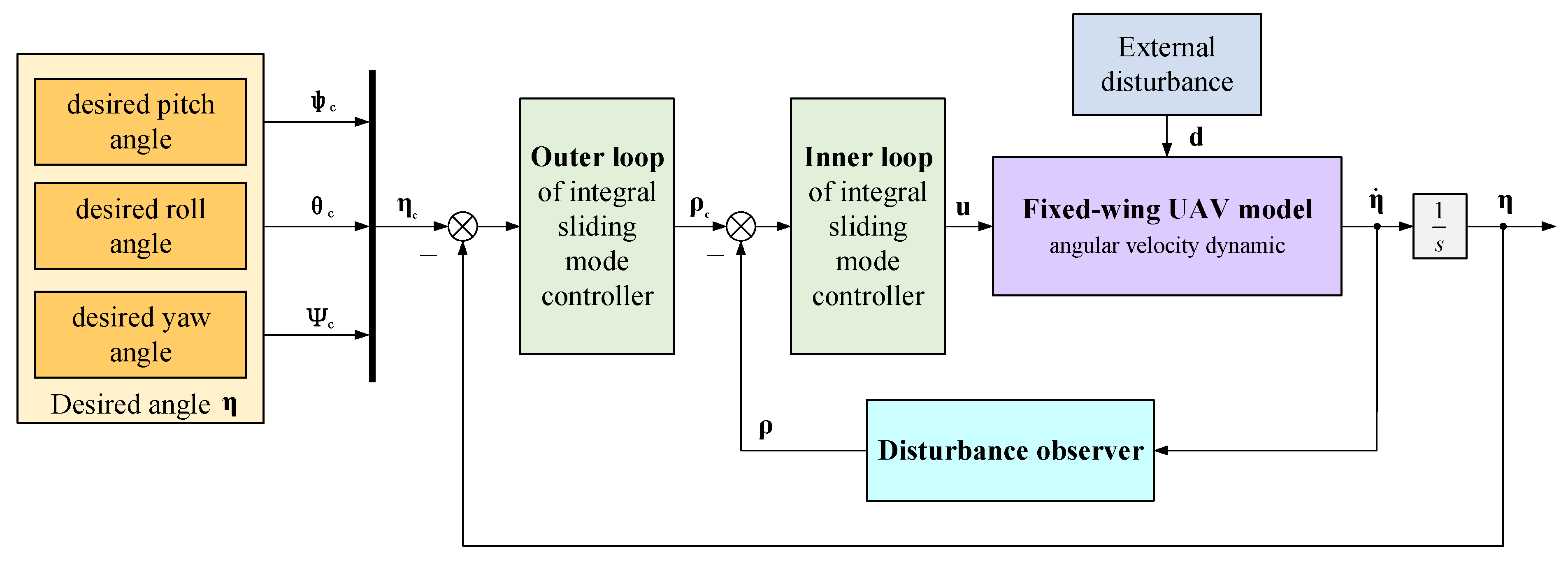
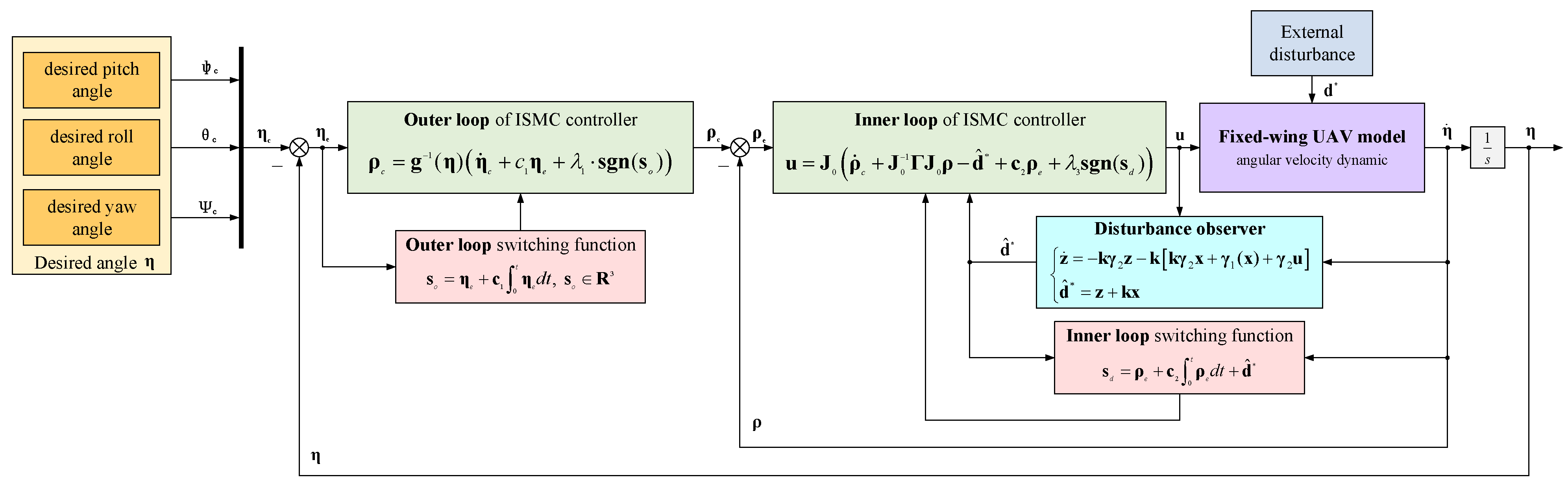
• A double-loop integral sliding mode control (ISMC) system is developed to accommodate attitude control amidst parameter uncertainties, such as fuel consumption during flight. An additional DO is integrated into the inner loop to estimate unpredictable external factors like sea-level wave disturbances. This composite integral sliding mode control based on disturbance observer (ISMC-DO) system not only achieves precise attitude control, but also fortifies the resistance of the UAV to external disturbances. The two-degrees-of-freedom controller predicated on ISMC-DO can effectively observe low-altitude wave disturbances, refine attitude tracking accuracy, and simultaneously ensure optimal tracking and anti-disturbance performance.
• While most studies traditionally rely on constant or square-wave instructions for attitude tracking, this paper diverges by employing ISMC-DO combined with the quaternion theory to track complex combat maneuver commands. To circumvent the singularity issues encountered during large-angle maneuvers, an outer loop for quaternion attitude control is formulated to acquire the desired angular velocity. Through extensive attitude tracking and aerobatic maneuver experiments, this paper validates the feasibility of executing complex combat maneuvers, such as looping, the split-S, and the Immelmann turn, thereby providing a theoretical and practical underpinning for high-precision combat maneuver tracking.

This paper is organized in the following manner. Section 2 establishes a fixed-wing UAV model with parameter uncertainties and establishes the control goal of this paper. Section 3 presents the ISMC-DO control method, along with proof of stability of the control system based on ISMC-DO. Then, experimental simulations and analysis are performed in Section 4. Some conclusions are obtained in Section 5.

2. Model Description

2.1. Modeling of Fixed-Wing UAV

Assume $o$ as the centroid for the fixed-wing UAV, and $oxyz$ as its body axis coordinate system. Based on Newton’s second law and the dynamics principle, the fixed-wing UAV nonlinear equation [36] is expressed as follows:

$$\left\{\begin{array}{l}\dot{\varphi }=v_p+\tan \theta (v_q\sin \varphi +v_r\cos \varphi )\\ \dot{\theta }=v_q\cos \varphi -v_r\sin \varphi \\ \dot{\psi }=(v_q\sin \varphi +v_r\cos \varphi )/\cos \theta \end{array}\right.$$

(1)

$$\left\{\begin{array}{l}(J_x+\Delta J_x)\dot{p}+\left((J_z+\Delta J_z)-(J_y+\Delta J_y)\right)qr=M_x\\ (J_y+\Delta J_y)\dot{q}+\left((J_x+\Delta J_x)-(J_z+\Delta J_z)\right)pr=M_y\\ (J_z+\Delta J_z)\dot{r}+\left((J_y+\Delta J_y)-(J_x+\Delta J_x)\right)pq=M_z\end{array}\right.$$

(2)

$$\left\{\begin{array}{l}\dot{x}=W\cos \chi \cos \gamma \\ \dot{y}=W\sin \chi \cos \gamma \\ \dot{z}=-W\sin \gamma \end{array}\right.$$

(3)

$$\left\{\begin{array}{l}{\dot{v}}_1=v_{r}v-v_{q}w+{\displaystyle \frac{\overline{X}+T-mg\sin \theta }{m}}\\ {\dot{v}}_2=v_{p}w-v_{r}u+{\displaystyle \frac{\overline{Y}+mg\sin \varphi \cos \theta }{m}}\\ {\dot{v}}_3=v_{q}u-v_{p}v+{\displaystyle \frac{\overline{Z}+mg\cos \varphi \cos \theta }{m}}\end{array}\right.$$

(4)

where $\varphi ,\theta ,\psi$ $(\mathrm{r}\mathrm{a}\mathrm{d})$ denote the roll, pitch, and yaw angles, respectively, with the roll, pitch, and yaw angular velocities being represented by $v_p,v_q,v_r$ $(\mathrm{m}/\mathrm{s})$, respectively; $I_{\varphi },I_{\theta },I_{\psi }$ $(\mathrm{k}\mathrm{g}/{\mathrm{m}}^2)$ are the moments of inertia matrix rotating around the centroid, and $\Delta I_{\varphi },\Delta I_{\theta },\Delta I_{\psi }$ $(\mathrm{k}\mathrm{g}/{\mathrm{m}}^2)$ are the uncertain parts of the inertia matrix; $M_x,M_y,M_z$ $(\mathrm{N}\cdot \mathrm{m})$ are the control moments; $v_1,v_2,v_3$ $(\mathrm{m}/\mathrm{s})$ are the velocities of the body axis coordinate system; $W$ $(\mathrm{m}/\mathrm{s})$ is the true air speed; $\chi ,\gamma$ $(\mathrm{r}\mathrm{a}\mathrm{d})$ are the azimuth angle and inclination angle in the flight path; and $\overline{X},\overline{Y},\overline{Z}$ $(\mathrm{N})$ are axial, lateral, and normal forces, respectively [37]. The assumptions made in the derivation of the control system are given in Assumptions 1 to 4 in Section 3.

2.2. Control Goal

The primary aim of this paper is to introduce a sophisticated anti-disturbance attitude control framework tailored for a dynamic equation that considers parameter uncertainties arising from variables such as fuel consumption and wave disturbances. The devised strategy seeks to optimize the tracking performance for both the attitude angle and its corresponding angular velocity.

• Initially, we introduce a double-closed-loop ISMC system designed to mitigate model uncertainties and decouple the relationships among the triad of attitude angles. Namely, the control goals are $\underset{t\to \infty }{\lim } s_{\theta }(t)=0$, $\underset{t\to \infty }{\lim } s_{\mathbf{\omega }}(t)=0$, so as to achieve $\underset{t\to \infty }{\lim }({\theta }_d-\theta )(t)=0$ and $\underset{t\to \infty }{\lim }({\mathbf{\omega }}_d-\mathbf{\omega })(t)=0$, where ${\theta }_d$ is the desired attitude angle vector, ${\mathbf{\omega }}_d$ is the desired angular velocity vector, $s_{\theta }(t)$ is the sliding surface of the attitude angle control loop, and $s_{\mathbf{\omega }}(t)$ is the sliding surface of the angular velocity control loop.
• In consideration of the impact that sea-level wave disturbances have on low-altitude attitude tracking, a DO is incorporated to estimate these unknown disturbances. Let the disturbance estimated by DO be $\widehat{d}(t)$. The goal of the DO is to minimize the estimation error $\tilde{d}(t)=d(t)-\widehat{d}(t)$.
• Finally, to ensure accurate tracking of specialized combat maneuvers, the challenges of singularity in large-angle maneuvers are addressed through the adoption of the quaternion theory for the outer loop of the attitude control system. Let the quaternion $\gamma ={\left[\begin{array}{cccc}{\gamma }_0& {\gamma }_1& {\gamma }_2& {\gamma }_3\end{array}\right]}^T$ describe the attitude, and the desired quaternion be ${\gamma }_d$. The quaternion tracking error is $e_{\gamma }={\gamma }_d^{-1}\otimes \gamma$. The control goal is that within the completion time $t_l$ of the large-angle maneuver, $\underset{t\to t_l}{\lim }‖e_{\gamma }‖\le \upsilon$, where $\upsilon$ is a given small positive number.

3. An Anti-Disturbance Attitude Control Method Based on ISMC-DO and Quaternions for Large-Angle Maneuvering Problems

3.1. Design of Integral Sliding Mode Controller Based on Disturbance Observer

Assuming that the attitude angle is $\eta ={[\varphi ,\theta ,\psi ]}^T$ and the angular velocity is $\rho ={[v_p,v_q,v_r]}^T$, the dynamic equation governing the rotation of the UAV around its centroid can be expressed accordingly:

$$\left\{\begin{array}{l}\dot{\eta }=g(\eta )\rho \\ (J_0+\Delta J)\dot{\rho }=-\Gamma (J_0+\Delta J)\rho +M+d\\ y=\eta \end{array}\right.$$

(5)

where the moment of inertia matrix of the UAV, rotating about its centroid, is represented by $J_0=diag\{I_{\varphi },I_{\theta },I_{\psi }\},J_0\in R^3$, and $\Delta J\in R^{3\times 3}$ is the uncertainty term caused by the inertia matrix due to reasons like fuel consumption. The matrix $\Gamma$ is defined as $\Gamma =\left(\begin{array}{ccc}0& -v_r& -v_q\\ v_r& 0& -v_p\\ -v_q& v_p& 0\end{array}\right)$ and the matrix $g(\eta )$ is defined as $g(\eta )=\left(\begin{array}{ccc}1& \tan \theta \sin \varphi & \tan \theta \cos \varphi \\ 0& \cos \varphi & -\sin \varphi \\ 0& {\displaystyle \frac{\sin \varphi }{\cos \theta }}& {\displaystyle \frac{\cos \varphi }{\cos \theta }}\end{array}\right)$.

Assumption 1.

The system disturbance $d$ is bounded within a known limit $D=\underset{t>0}{\sup }|d(t)|$.

Assumption 2.

Except for some states whose measurements are subject to noise and uncertainties, the measured values of most states can be promptly fed back into the control system.

Based on Equation (5), the following equation can be derived:

$$\begin{array}{l}{J}_0\dot{\rho }=-\Gamma J_0\rho -\Gamma \Delta J\rho +M+d-\Delta J\dot{\rho }\\ \ddot{\eta }=\dot{g}(\eta )\rho +g(\eta )\dot{\rho }\Rightarrow \dot{\rho }=g^{-1}(\eta )\left(\ddot{\eta }-\dot{g}(\eta )\rho \right)\end{array}$$

(6)

Let $x={\left[x_1,x_2\right]}^T={\left[\eta ,\rho \right]}^T$, $u=M$, we can obtain:

$$\left\{\begin{array}{l}\dot{x}={\gamma }_1(x)+{\gamma }_{2}u+{\gamma }_{2}d\\ y=x_1\end{array}\right.$$

(7)

where ${\gamma }_1(x)={\left[g(\eta )\rho ,-{(J_0+\Delta J)}^{-1}\Gamma (J_0+\Delta J)\rho \right]}^T$, ${\gamma }_2={\left[0,{(J_0+\Delta J)}^{-1}\right]}^T$.

The attitude control of the UAV is orchestrated through a double-closed-loop ISMC system. Given the target attitude angles, the outer loop produces an attitude angular velocity instruction ${\rho }_c$, which is conveyed to the inner loop system. The inner loop then tracks this angular velocity instruction ${\rho }_c$ via its own ISMC protocol. Figure 1 illustrates the anti-disturbance attitude control structure based on ISMC, wherein the outer loop represents the position ring, and the inner loop serves as the velocity ring equipped with a DO.

Let ${\rho }_c$ denote the control input for the outer loop tasked with tracking the angle $\eta$. With the tracking instruction deviation represented by ${\eta }_e={\eta }_c-\eta$, the sliding mode function of the outer loop can be expressed mathematically, as follows:

$$s_o={\eta }_e+c_1{\displaystyle {\int }_0^t{\eta }_e}dt, s_o\in R^3$$

(8)

where $c_1=diag\{c_{11},c_{12},c_{13}\}$ is the gain matrix. The tracking error of the system can be stabilized on an ideal sliding mode by selecting a suitable gain matrix.

The attitude angular velocity instruction ${\rho }_c$ serves as a virtual control term for tracking the attitude angular velocity $\rho$. Any discrepancies between ${\rho }_c$ and $\rho$ are rectified by the inner loop controller. The attitude angular velocity instruction is designed as follows:

$$\rho =g^{-1}(\eta )\left({\dot{\eta }}_c+c_1{\eta }_e+{\lambda }_1\cdot sgn(s_o)\right)$$

(9)

where $sgn(s_o)={[\begin{array}{ccc}\mathrm{sgn}(s_1)& \mathrm{sgn}(s_2)& \mathrm{sgn}(s_3)\end{array}]}^T$, ${\lambda }_1>0$.

It can be obtained from Equation (8) that

$${\dot{s}}_o={\dot{\eta }}_e+c_1{\eta }_e={\dot{\eta }}_c-\dot{\eta }+c_1{\eta }_e={\dot{\eta }}_c-g(\eta )\rho +c_1{\eta }_e$$

(10)

The following Lyapunov function is designed:

$$V={\displaystyle \frac{1}{2}}{s}_o^T{s}_o$$

(11)

then:

$$\begin{array}{l}\dot{V}=s_o^T{\dot{s}}_o=s_o^T\left({\dot{\eta }}_c-g(\eta )\rho +c_1{\eta }_e\right)\\ =s_o^T\left\{{\dot{\eta }}_c-g(\eta )\left[g^{-1}(\eta )\left({\dot{\eta }}_c+c_1{\eta }_e+{\lambda }_1\cdot sgn(s_o)\right)\right]+c_1{\eta }_e\right\}\\ =-{\lambda }_1{s}_o^{T}sgn(s_o)=-{\lambda }_1\underset{i=1}{\overset{3}{\Sigma }}\left|s_{oi}\right|<0\end{array}$$

(12)

As shown in Figure 1, in order to realize ${\rho }_c\to \rho$, the ISMC law $M$ of the inner loop is designed so that ${\rho }_c-\rho \to 0$, namely, the following equation is established:

$$\underset{t\to \infty }{\lim }‖\rho -{\rho }_c‖=0$$

(13)

Figure 1. Anti-disturbance attitude control block diagram based on ISMC.

Figure 1. Anti-disturbance attitude control block diagram based on ISMC.

Let the deviation of the attitude angular velocity instruction be ${\rho }_e={\rho }_c-\rho$; the ISMC function of the inner loop is expressed as follows:

$$s_l={\rho }_e+c_2{\displaystyle {\int }_0^t{\rho }_e}dt, s_l\in R^3$$

(14)

where $c_2=diag\{c_{21},c_{22},c_{23}\}$ is the gain matrix.

The design of the control law is formulated as follows:

$$M=J_0{\dot{\rho }}_c+J_0{c}_2{\rho }_e+\Gamma J_0\rho +\mu s_l+{\lambda }_{2}sgn(s_l)$$

(15)

where $\mu >0$, and ${\lambda }_2>0$.

Equations (5) and (14) yield the following:

$$\begin{array}{l}{\dot{s}}_l={\dot{\rho }}_e+c_2{\rho }_e={\dot{\rho }}_c-\dot{\rho }+c_2{\rho }_e\\ ={\dot{\rho }}_c+{(J_0+\Delta J)}^{-1}\Gamma (J_0+\Delta J)\rho -{(J_0+\Delta J)}^{-1}M-{(J_0+\Delta J)}^{-1}d+c_2{\rho }_e\end{array}$$

(16)

The following Lyapunov function is designed:

$$V={\displaystyle \frac{1}{2}}{s}_l^T(J_0+\Delta J)s_l$$

(17)

where $(J_0+\Delta J)$ is a positive definite matrix, so $V>0$, then

$$\begin{array}{l}\dot{V}=s_l^T\left[\Delta \dot{J}{s}_l/2+(J_0+\Delta J){\dot{s}}_l\right]\\ =s_l^T\Delta \dot{J}{s}_l/2+s_l^T(J_0+\Delta J)[{\dot{\rho }}_c+{(J_0+\Delta J)}^{-1}\Gamma (J_0+\Delta J)\rho -{(J_0+\Delta J)}^{-1}M\\ -{(J_0+\Delta J)}^{-1}d+c_2{\rho }_e]\\ =s_l^T\Delta \dot{J}{s}_l/2+s_l^T[(J_0+\Delta J){\dot{\rho }}_c+\Gamma (J_0+\Delta J)\rho -M-d+(J_0+\Delta J)c_2{\rho }_e]\end{array}$$

(18)

Common sense tells us that $s_l^T{s}_l={‖s_l‖}^2,s_l^{T}sgn(s_l)=\underset{i=1}{\overset{3}{\Sigma }}\left|s_{li}\right|$. By substituting Equation (15) into Equation (18), one obtains the following:

$$\begin{array}{l}\dot{V}=s_l^T\Delta \dot{J}{s}_l/2+s_l^T[(J_0+\Delta J){\dot{\rho }}_c+\Gamma (J_0+\Delta J)\rho -J_0{\dot{\rho }}_c-J_0{c}_2{\rho }_e\\ -\Gamma J_0\rho -\mu s_l-{\lambda }_{2}sgn(s_l)-d+(J_0+\Delta J)c_2{\rho }_e]\\ =s_l^T\Delta \dot{J}{s}_l/2+s_l^T\left[\Delta J{\dot{\rho }}_c+\Gamma \Delta J\rho -\mu s_l-{\lambda }_{2}sgn(s_l)-d+\Delta J{c}_2{\rho }_e\right]\\ =s_l^T\Delta \dot{J}{s}_l/2+s_l^T\left[\Delta J{\dot{\rho }}_c+\Gamma \Delta J\rho -d+\Delta J{c}_2{\rho }_e\right]-s_l^T\cdot [\mu s_l+{\lambda }_{2}sgn(s_l)]\\ =s_l^T\Delta \dot{J}{s}_l/2+s_l^T\left[\Delta J{\dot{\rho }}_c+\Gamma \Delta J\rho -d+\Delta J{c}_2{\rho }_e\right]-\mu {‖s_l‖}^2-{\lambda }_2\underset{i=1}{\overset{3}{\Sigma }}\left|s_{li}\right|\end{array}$$

(19)

Assuming that the uncertain terms $\Delta J$ and $d$ are bounded, the following equation can be obtained:

$${\left|\Delta J{\dot{\rho }}_c+\Gamma \Delta J\rho -d+\Delta J{c}_2{\rho }_e\right|}_i\le {\lambda }_i\le {\lambda }_2, i=1,2,3$$

(20)

Supposing that ${\lambda }_{\max }$ is the maximum eigenvalue of $\Delta \dot{J}$, and by designing $\mu$, $\mu -{\lambda }_{\max }>0$, then

$$\dot{V}\le -(\mu -{\lambda }_{\max }){‖s_l‖}^2\le 0$$

(21)

When faced with significant modeling uncertainties and external disturbances, it may be tempting to elevate the switching gain value in the ISMC controller. However, doing so may introduce chattering—an undesirable side effect. To circumvent this issue, the ISMC employs the saturation function $\mathrm{sat}(\mathrm{s})$ as a replacement for the symbolic function $\mathrm{sgn}(\mathrm{s})$:

$$\mathrm{sat}(\mathrm{s})=\left\{\begin{array}{ll}1,& s>\Delta \\ ks,& \left|s\right|\le \Delta \\ -1,& s<-\Delta \end{array}\right.$$

(22)

where $\Delta$ is the boundary layer.

Remark 1.

It is crucial to differentiate between critical stability and engineering stability. While the positive-definite nature of $V$ and its semi-negative-definite derivative $\dot{V}$ in Equations (17) and (21) suggest critical stability, they fall short of demonstrating engineering stability. For a comprehensive discussion on asymptotic stability in an engineering context, we proceed as follows.

Invoking the corollary of Barbalat’s Lemma [38] (if $\Gamma (t)$ is a differentiable function, when $t\to \infty$, there is a finite limit, and $\ddot{\Gamma }$ exists and is bounded), we find that $\Gamma (t)\to 0$ when $t\to \infty$. According to Equation (21), the energy error is obtained as follows:

$${\displaystyle \int s^2(t)dt=}{\displaystyle \frac{1}{{\lambda }_2}}\left[V\left(s(0),\Delta J(0),d(0)\right)-V\left(s(\infty ),\Delta J(\infty ),d(\infty )\right)\right]<\infty$$

(23)

The corollary of Barbalat’s Lemma shows that $s(t)$ is a decreasing function, so when $s(t)\to \infty$ is satisfied, $\dot{V}<0$ is established. Therefore, for Lyapunov functions with semi-negative-definite derivatives, the conclusion that the system is asymptotically stable in engineering can be obtained according to the corollary.

System (5) is expressed as follows:

$$\begin{array}{l}\dot{\rho }=-J_0^{-1}\Gamma J_0\rho +J_0^{-1}M+J_0^{-1}d-J_0^{-1}\Gamma \Delta J\rho -J_0^{-1}\Delta J\dot{\rho }\\ \triangleq -J_0^{-1}\Gamma J_0\rho +J_0^{-1}u+d^{\ast }\\ \dot{\eta }=g(\eta )\rho \end{array}$$

(24)

If the unmatched disturbance $d^{\ast }$ of Equation (24) is assumed to be bounded, then it can be estimated by employing a nonlinear DO [39]. The mathematical representation of the DO is as follows:

$$\left\{\begin{array}{l}\dot{z}=-k{\gamma }_{2}z-k\left[k{\gamma }_{2}x+{\gamma }_1(x)+{\gamma }_{2}u\right]\\ {\widehat{d}}^{\ast }=z+kx\end{array}\right.$$

(25)

where ${\widehat{d}}^{\ast }$ is the estimate of the unmatched disturbance, $z$ is the DO’s internal state, and $k$ is the designed observer gain. By designing the function $k$, ${\widehat{d}}^{\ast }$ approximates the unmatched disturbance $d^{\ast }$ exponentially.

For sliding mode control, disturbances may cause the system state to deviate from the sliding mode surface or deteriorate the control effect. When designing the sliding mode function $s_d$, adding ${\widehat{d}}^{\ast }$ in Equation (25) can offset the influence of $d^{\ast }$ to a certain extent, enabling the system to still track the desired state well in the presence of disturbances.

$$s_d={\rho }_e+c_2{\displaystyle {\int }_0^t{\rho }_e}dt+{\widehat{d}}^{\ast }$$

(26)

where ${\widehat{d}}^{\ast }$ denotes the disturbance estimate in Equation (25). The parameter to be designed for control is $c_2$.

The design of the ISMC-DO control law is formulated as follows:

$$u=J_0\left({\dot{\rho }}_c+J_0^{-1}\Gamma J_0\rho -{\widehat{d}}^{\ast }+c_2{\rho }_e+{\lambda }_{3}sgn(s_d)\right)$$

(27)

where ${\lambda }_3$ is the designed switching gain. The attitude control structure based on ISMC-DO is shown in Figure 2 below.

Remark 2.

Importantly, the switching gain in the ISMC-DO controller need only surpass the boundary of the disturbance observation error—not the actual disturbance. Consequently, this allows for a reduction in switching gain, which in turn minimizes chattering and enhances the stable flight performance of fixed-wing UAVs.

The subsequent stability analysis of the control system, leveraging ISMC-DO, will be expounded upon in Section 3.3.

3.2. Attitude Controller Based on Quaternions for Combat Maneuvers

Trigonometric functions and singular points are intrinsic features of the attitude kinematics model formulated through Euler angles. Consequently, the utility of this model is predominantly confined to the management and stabilization of attitude for minor angular deviations. Nonetheless, in large maneuvers with a pitch angle $\theta$ of 90° or −90°, the Euler angle representation method exhibits singularity, causing sudden changes in the roll angle $\dot{\varphi }$ and yaw angle $\dot{\psi }$ during calculation. When $\theta$ is 90° or −90°, $\cos \theta$ equals zero, and $\tan \theta$ is infinite, then it fails to be calculated, indicating the occurrence of singularity. The sudden shift in attitude angle at singular points leads to a rapid alteration in angular velocity, thereby negatively impacting the stability of UAVs during real-world operations. To address the issues of singularity inherent to the Euler angle model, the adoption of quaternions [40] has been proposed. Unlike Euler angles, quaternions are devoid of singularities and serve to mitigate the nonlinearity of the problem. Consequently, the use of quaternions has gained prominence for tackling the complexities linked with maneuvering at large angles.

The quaternion is defined as $\gamma =\left[\begin{array}{cccc}{\gamma }_0& {\gamma }_1& {\gamma }_2& {\gamma }_3\end{array}\right]=\left[\begin{array}{cc}{\gamma }_0& {\gamma }_v\end{array}\right]$, which satisfies the following constraint equation:

$${\gamma }_0^2+{\gamma }_1^2+{\gamma }_2^2+{\gamma }_3^2=1$$

(28)

The relationship between the quaternion and Euler angle is as follows:

$$\left[\begin{array}{l}{\gamma }_0\\ {\gamma }_1\\ {\gamma }_2\\ {\gamma }_3\end{array}\right]=\left[\begin{array}{l}\cos (\varphi /2)\cos (\theta /2)\cos (\psi /2)+\sin (\varphi /2)\sin (\theta /2)\sin (\psi /2)\\ \sin (\varphi /2)\cos (\theta /2)\cos (\psi /2)-\cos (\varphi /2)\sin (\theta /2)\sin (\psi /2)\\ \cos (\varphi /2)\sin (\theta /2)\cos (\psi /2)+\sin (\varphi /2)\cos (\theta /2)\sin (\psi /2)\\ \cos (\varphi /2)\cos (\theta /2)\sin (\psi /2)-\sin (\varphi /2)\sin (\theta /2)\cos (\psi /2)\end{array}\right]$$

(29)

$$\begin{array}{l}\theta =-\arcsin \left(2{\gamma }_1{\gamma }_3-2{\gamma }_0{\gamma }_2\right)\\ \varphi =-\arctan 2\left({\displaystyle \frac{2({\gamma }_2{\gamma }_3-{\gamma }_0{\gamma }_1)}{1-2({\gamma }_1^2+{\gamma }_2^2)}}\right)\\ \psi =-\arctan 2\left({\displaystyle \frac{2({\gamma }_1{\gamma }_2-{\gamma }_0{\gamma }_3)}{1-2({\gamma }_2^2+{\gamma }_3^2)}}\right)\end{array}$$

(30)

where the function $\arctan 2$ is calculated as follows:

$$\arctan 2(y,x)=\left\{\begin{array}{ll}\arctan {\displaystyle \frac{y}{x}},& x>0\\ \arctan {\displaystyle \frac{y}{x}}+\pi ,& y\ge 0,x<0\\ \arctan {\displaystyle \frac{y}{x}}-\pi ,& y<0,x<0\\ {\displaystyle \frac{1}{2}}\pi ,& y>0,x=0\\ -{\displaystyle \frac{1}{2}}\pi ,& y<0,x=0\\ \mathrm{undefined},& y=0,x=0\end{array}\right.$$

(31)

where the value range of the function is $[-\pi ,\pi ]$.

Using quaternions to replace the Euler angle, one obtains the following:

$$\begin{array}{l}{\dot{v}}_1=v_r{v}_2-v_q{v}_3+{\displaystyle \frac{2({\gamma }_1{\gamma }_3-{\gamma }_0{\gamma }_2)mg+\overline{X}+T}{m}}\\ {\dot{v}}_2=v_{p}w-v_r{v}_1+{\displaystyle \frac{2({\gamma }_2{\gamma }_3+{\gamma }_0{\gamma }_1)mg+\overline{Y}}{m}}\\ {\dot{v}}_3=v_q{v}_1-v_p{v}_2+{\displaystyle \frac{2({\gamma }_0^2-{\gamma }_1^2-{\gamma }_2^2+{\gamma }_3^2)mg+\overline{Z}}{m}}\end{array}$$

(32)

$$\left[\begin{array}{l}\dot{x}\\ \dot{y}\\ \dot{z}\end{array}\right]=\left[\begin{array}{ccc}{\gamma }_0^2+{\gamma }_1^2-{\gamma }_2^2-{\gamma }_3^2& 2({\gamma }_1{\gamma }_2-{\gamma }_0{\gamma }_3)& 2({\gamma }_1{\gamma }_3+{\gamma }_0{\gamma }_2)\\ 2({\gamma }_1{\gamma }_2+{\gamma }_0{\gamma }_3)& {\gamma }_0^2-{\gamma }_1^2+{\gamma }_2^2-{\gamma }_3^2& 2({\gamma }_2{\gamma }_3-{\gamma }_0{\gamma }_1)\\ 2({\gamma }_1{\gamma }_3-{\gamma }_0{\gamma }_2)& 2({\gamma }_2{\gamma }_3+{\gamma }_0{\gamma }_1)& {\gamma }_0^2-{\gamma }_1^2-{\gamma }_2^2+{\gamma }_3^2\end{array}\right]\left[\begin{array}{l}{v}_1\\ v_2\\ v_3\end{array}\right]$$

(33)

The relationship between the quaternion and angular velocity is as follows:

$$\dot{\gamma }=\left[\begin{array}{l}{\dot{\gamma }}_0\\ {\dot{\gamma }}_1\\ {\dot{\gamma }}_2\\ {\dot{\gamma }}_3\end{array}\right]={\displaystyle \frac{1}{2}}\left[\begin{array}{cccc}0& -v_p& -v_q& -v_r\\ v_p& 0& v_r& -v_q\\ v_q& -v_r& 0& v_p\\ v_r& v_q& -v_p& 0\end{array}\right]\left[\begin{array}{l}{\gamma }_0\\ {\gamma }_1\\ {\gamma }_2\\ {\gamma }_3\end{array}\right]$$

(34)

Rewriting Equation (34) yields the following:

$$\dot{\gamma }=\left[\begin{array}{l}{\dot{\gamma }}_0\\ {\dot{\gamma }}_1\\ {\dot{\gamma }}_2\\ {\dot{\gamma }}_3\end{array}\right]={\displaystyle \frac{1}{2}}\left[\begin{array}{ccc}-{\gamma }_1& -{\gamma }_2& -{\gamma }_3\\ {\gamma }_0& -{\gamma }_3& {\gamma }_2\\ {\gamma }_3& {\gamma }_0& -{\gamma }_1\\ -{\gamma }_2& {\gamma }_1& {\gamma }_0\end{array}\right]\left[\begin{array}{l}{v}_p\\ v_q\\ v_r\end{array}\right]$$

(35)

The outer loop employs quaternion attitude control, designed in accordance with Equation (35). The desired angular velocity is computed based on both the quaternion command and the quaternion feedback of the UAV. This calculated velocity is subsequently controlled by the dedicated angular velocity ring.

3.3. Stability Analysis

Assumption 3.

In Equation (24), the derivative ${\dot{d}}^{\ast }$ of the disturbance is bounded and satisfied $\underset{t\to \infty }{\lim } {\dot{d}}^{\ast }=0$.

Lemma 1.

Assume that the system (24) satisfies Assumptions 1 and 3. Following selection of the appropriate observer gain $k>0$, the DO estimation ${\widehat{d}}^{\ast }$ in (25) can asymptotically track the disturbance $d^{\ast }$ of system (24) [41], so that

$${\dot{\tilde{d}}}^{\ast }(t)+k{\tilde{d}}^{\ast }(t)=0$$

(36)

is globally stable, where ${\tilde{d}}^{\ast }=d^{\ast }-{\widehat{d}}^{\ast }$ is the error of the disturbance estimate.

Assumption 4.

In (36), the disturbance estimation error is confined within $D^{\ast }=\underset{t>0}{\sup }|{\tilde{d}}^{\ast }(t)|$.

Lemma 2.

Consider $\dot{\rho }=f(\rho ,u)$ to be a nonlinear system displaying input-to-state stability. If the input complies with the condition $\underset{t\to \infty }{\lim }u(t)=0$, then the state $\underset{t\to \infty }{\lim }\rho (t)=0$ is deduced.

Theorem 1.

For the uncertain nonlinear system (5), under the condition that the system assumptions hold, the nonlinear disturbance observer (25) estimates the unmatched disturbance $d^{\ast }$ by designing the observer gain $k$. The switching gain ${\lambda }_3$ in the control law (27) is designed as ${\lambda }_3>(k-1)D^{\ast }$ and an appropriate observer gain $k$ is chosen so that $k>0$; thus, the closed-loop system is asymptotically stable.

Proof. 

By taking the derivative of the sliding mode function $s_d$ of (26), and combining Equations (24) and (27), one obtains the following:

$$\begin{array}{l}{\dot{s}}_d={\dot{\rho }}_e+c_2{\rho }_e+{\dot{\widehat{d}}}^{\ast }={\dot{\rho }}_c-\dot{\rho }+c_2{\rho }_e+{\dot{\widehat{d}}}^{\ast }\\ ={\dot{\rho }}_c-(-J_0^{-1}\Gamma J_0\rho +J_0^{-1}u+d^{\ast })+c_2{\rho }_e+{\dot{\widehat{d}}}^{\ast }\\ ={\dot{\rho }}_c+J_0^{-1}\Gamma J_0\rho -J_0^{-1}[J_0({\dot{\rho }}_c+J_0^{-1}\Gamma J_0\rho -{\widehat{d}}^{\ast }+c_2{\rho }_e+{\lambda }_{3}sgn(s_d))]-d^{\ast }+c_2{\rho }_e+{\dot{\widehat{d}}}^{\ast }\\ =-{\lambda }_{3}sgn(s_d)-(d^{\ast }-{\widehat{d}}^{\ast })+{\dot{\widehat{d}}}^{\ast }\end{array}$$

(37)

It can be obtained from Equation (25) that

$$\begin{array}{l}{\dot{\widehat{d}}}^{\ast }=\dot{z}+k\dot{\rho }=-kz-k(k\rho -J_0^{-1}\Gamma J_0\rho +J_0^{-1}u)+k\dot{\rho }\\ =-kz-k(k\rho +\dot{\rho }-d^{\ast })+k\dot{\rho }\\ =-k({\widehat{d}}^{\ast }-d^{\ast })\end{array}$$

(38)

Substituting Equation (38) into (37) yields the following:

$$\begin{array}{ll}{\dot{s}}_d& =-{\lambda }_{3}sgn(s_d)-(d^{\ast }-{\widehat{d}}^{\ast })+k(d^{\ast }-{\widehat{d}}^{\ast })\\ & =-{\lambda }_{3}sgn(s_d)+(k-1)(d^{\ast }-{\widehat{d}}^{\ast })\\ & =-{\lambda }_{3}sgn(s_d)+(k-1){\tilde{d}}^{\ast }\end{array}$$

(39)

Consider the following Lyapunov function:

$$V={\displaystyle \frac{s_d^2}{2}}$$

(40)

When $s_d>0$, $s_{d}sgn(s_d)=s_d$; when $s_d<0$, $s_{d}sgn(s_d)=\left|s_d\right|$, so $s_{d}sgn(s_d)=\left|s_d\right|$. By taking the derivative of Equation (40) and combining it with Equation (39), one obtains the following:

$$\begin{array}{l}\dot{V}=s_d{\dot{s}}_d=[-{\lambda }_{3}sgn(s_d)+(k-1){\tilde{d}}^{\ast }]\cdot s_d\\ =-{\lambda }_3\left|s_d\right|+(k-1){\tilde{d}}^{\ast }{s}_d\\ \le -\left({\lambda }_3-(k-1)D^{\ast }\right)\left|s_d\right|\\ =-\sqrt{2}\left({\lambda }_3-(k-1)D^{\ast }\right)\sqrt{V}\end{array}$$

(41)

Under the conditions ${\lambda }_3>(k-1)D^{\ast }$ outlined in Theorem 1, the system state will intersect the sliding mode surface defined by Equation (26) within a finite time span, and it can be deduced from $s_d=0$ that

$$\rho =-c_2{\displaystyle {\int }_0^t\rho }dt+{\rho }_c+c_2{\displaystyle {\int }_0^t{\rho }_c}dt+{\widehat{d}}^{\ast }$$

(42)

By combining the dynamic characteristics of (42) and observer (25), one obtains the following:

$$\left\{\begin{array}{l}\dot{\rho }=-c_2\rho +{\dot{\rho }}_c+c_2{\rho }_c+k{\tilde{d}}^{\ast }\\ {\dot{\tilde{d}}}^{\ast }={\dot{d}}^{\ast }-k{\tilde{d}}^{\ast }\end{array}\right.$$

(43)

Given that the prior knowledge of the derivative of the disturbance $d^{\ast }$ is unattainable, we assume that the disturbance varies slowly compared to the dynamic characteristics of the observer, denoted as ${\dot{d}}^{\ast }=0$. Considering the given condition $k>0$, it can be proved that the following system is asymptotically stable:

$$\left\{\begin{array}{l}\dot{\rho }=-c_2\rho +{\dot{\rho }}_c+c_2{\rho }_c+k{\tilde{d}}^{\ast }\\ {\dot{\tilde{d}}}^{\ast }=-k{\tilde{d}}^{\ast }\end{array}\right.$$

(44)

According to the existing literature [37], the system (43) exhibits input-to-state stability. By integrating the conditions set forth in Assumption 3 and Lemma 2, it becomes evident that the state of the system (43) satisfies constraints $\underset{t\to \infty }{\lim }\dot{\rho }(t)=0$ and $\underset{t\to \infty }{\lim }{\tilde{d}}^{\ast }(t)=0$. Thus, based on the formulated control law, the system state will asymptotically gravitate towards the desired equilibrium point.□

Remark 3.

To ensure system stability, the switching gains for the ISMC and ISMC-DO controllers should be designed as ${\lambda }_1>\left|d^{\ast }\right|$, ${\lambda }_2>\left|d^{\ast }\right|$, and ${\lambda }_3>(k-1)|d^{\ast }-{\widehat{d}}^{\ast }|$. The switching gain values in the designed controllers are expected to be considerably lower than those in the $\underset{t\to \infty }{\lim }{\tilde{d}}^{\ast }(t)=0$ traditional SMC and ISMC controllers, thereby mitigating the issue of chattering. Owing to the capability of the DO for precise disturbance estimation, it is anticipated that the estimation error $|d^{\ast }-{\widehat{d}}^{\ast }|$ will converge to zero, thus keeping it substantially below the magnitude of $d^{\ast }$ [38].

Remark 4.

When there is no disturbance, the following equation can be derived from Equation (38):

$${\dot{\widehat{d}}}^{\ast }(t)=-k{\widehat{d}}^{\ast }(t)$$

(45)

When the initial value for the disturbance estimation is chosen as ${\widehat{d}}^{\ast }(0)=0$, then the condition ${\widehat{d}}^{\ast }(t)\equiv 0$ is satisfied. Consequently, the sliding mode function (26) and control law (27) described herein can be simplified to mimic the ISMC function and control law when no disturbance is present, thereby maintaining nominal control performance. Simulation results corroborate the enhanced attributes of the ISMC-DO controller.

4. Simulation

Utilizing various methods, such as ISMC, dynamic inverse control [42], and ISMC-DO, we successfully evaluated the efficacy of attitude control for fixed-wing UAVs. Comparative simulations were conducted using MATLAB/Simulink. For the aircraft simulations, specific weight characteristics and dimensional parameters of the UAV were indispensable.

Table 1. Parameters of F-16.

Parameter	Symbol	Value	Unit
Quality	$m$	9296.13	$\mathrm{k}\mathrm{g}$
Pneumatic reference area	$S_c$	27.64	${\mathrm{m}}^2$
Average aerodynamic chord length	$l_{av}$	3.37	$\mathrm{m}$
Reference wingspan	$l$	9.232	$\mathrm{m}$
Moment of inertia of pitch axis	$I_{\theta }$	12,875.2	$\mathrm{k}\mathrm{g}/{\mathrm{m}}^2$
Moment of inertia of roll axis	$I_{\varphi }$	75,674.1	$\mathrm{k}\mathrm{g}/{\mathrm{m}}^2$
Moment of inertia of yaw axis	$I_{\psi }$	85,552.7	$\mathrm{k}\mathrm{g}/{\mathrm{m}}^2$
Pitch axis inertia matrix change	$\Delta I_{\theta }$	800	$\mathrm{k}\mathrm{g}/{\mathrm{m}}^2$
Roll axis inertia matrix change	$\Delta I_{\varphi }$	900	$\mathrm{k}\mathrm{g}/{\mathrm{m}}^2$
Yaw axis inertia matrix change	$\Delta I_{\psi }$	1000	$\mathrm{k}\mathrm{g}/{\mathrm{m}}^2$

presents the relevant parameters of the F-16. Notably, the control surfaces of the F-16 are actuated by servo-controlled systems, which follow directives from the flight control system. It is important to mention that the model omits features like differential lift deflection, trailing-edge flaps, landing gear, and speed brakes, due to the unavailability of public data.

Table 2. Rudder position limits and speed limits for F-16.

Parameter	Location Limit	Unit	Rate limit	Unit
Elevator	$[-5\pi /36,+5\pi /36]$	$\mathrm{rad}$	$\pm \pi /3$	$\mathrm{rad}/\mathrm{s}$
Aileron	$[-43\pi /360,+43\pi /360]$	$\mathrm{rad}$	$\pm 4\pi /9$	$\mathrm{rad}/\mathrm{s}$
Rudder	$[-\pi /6,+\pi /6]$	$\mathrm{rad}$	$\pm 2\pi /3$	$\mathrm{rad}/\mathrm{s}$
Leading edge flap	$[0,+5\pi /36]$	$\mathrm{rad}$	$\pm 5\pi /36$	$\mathrm{rad}/\mathrm{s}$

delineates the limitations regarding rudder position and speed for the F-16, while

Table 3. ISMC-DO controller parameters.

Parameter	Symbol	Value
Parameters of ISMC inner loop	$c_1$	$diag\{0.27,0.27,0.27\}$
	${\lambda }_1$	6.5
Parameters of ISMC outer loop	$c_2$	$diag\{1,1,1\}$
	${\lambda }_2$	2
Parameters of DO	$k_0$	3
	${\lambda }_3$	5

discloses the parameters of both the inner and outer loops of the ISMC controller, as well as the disturbance observer.

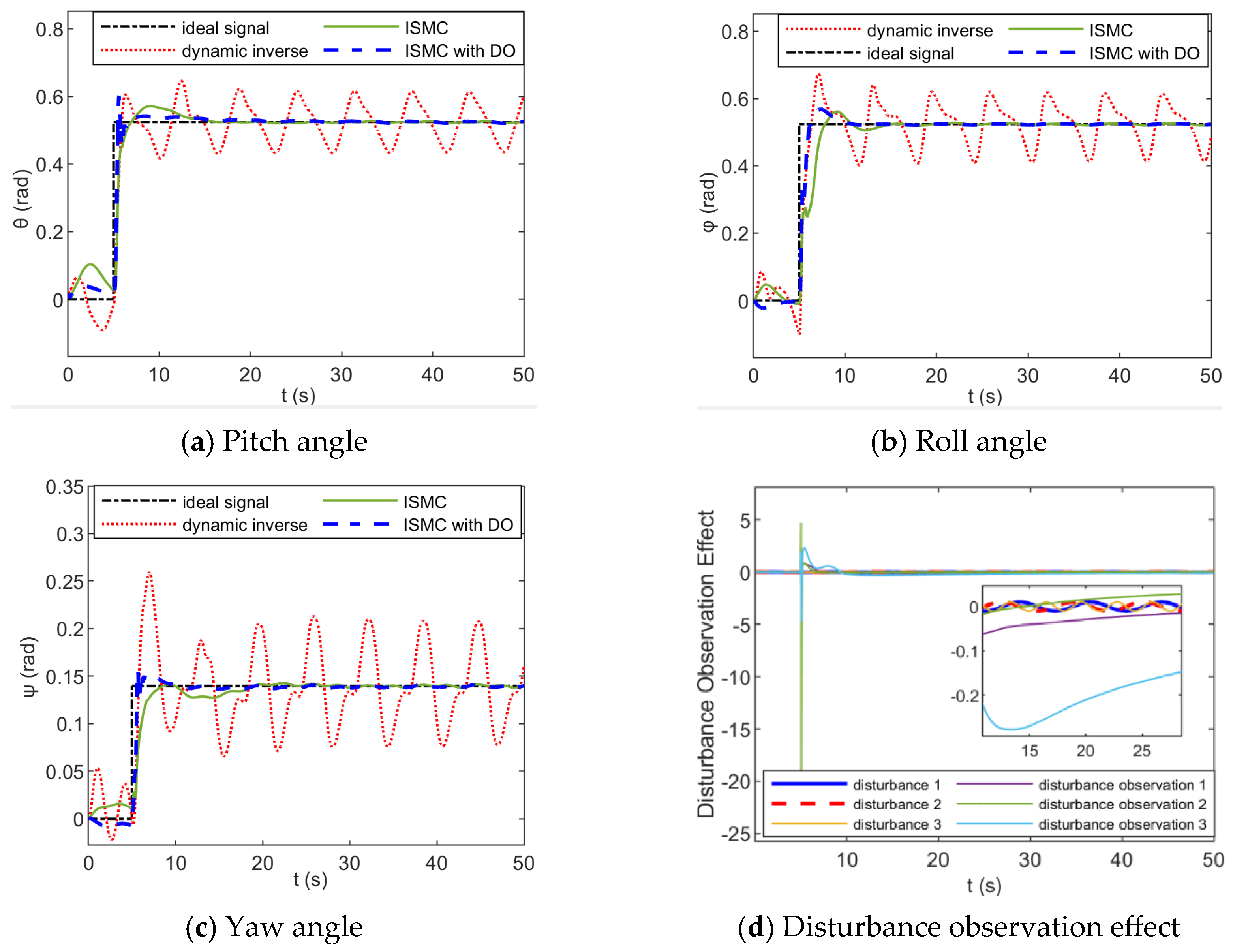
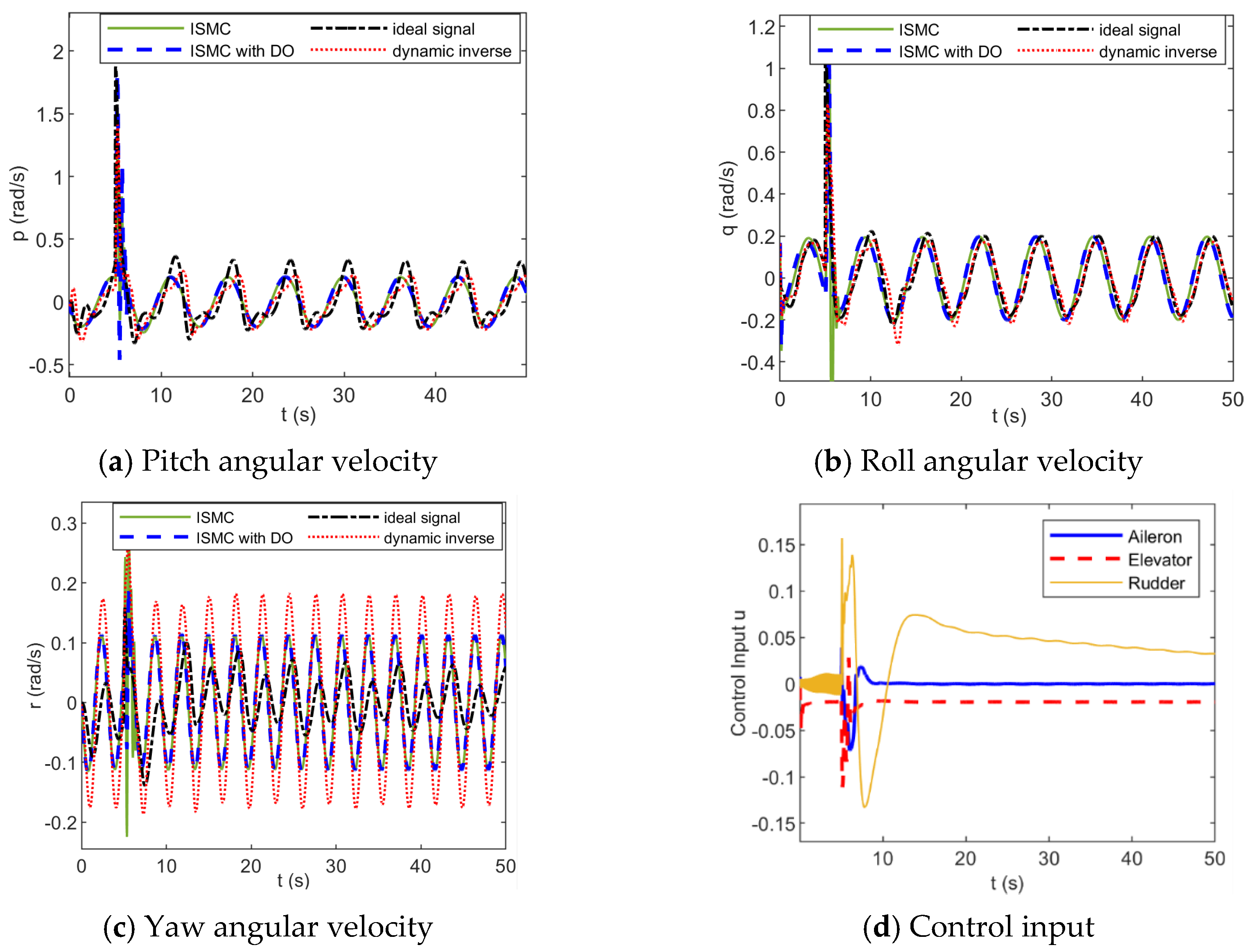
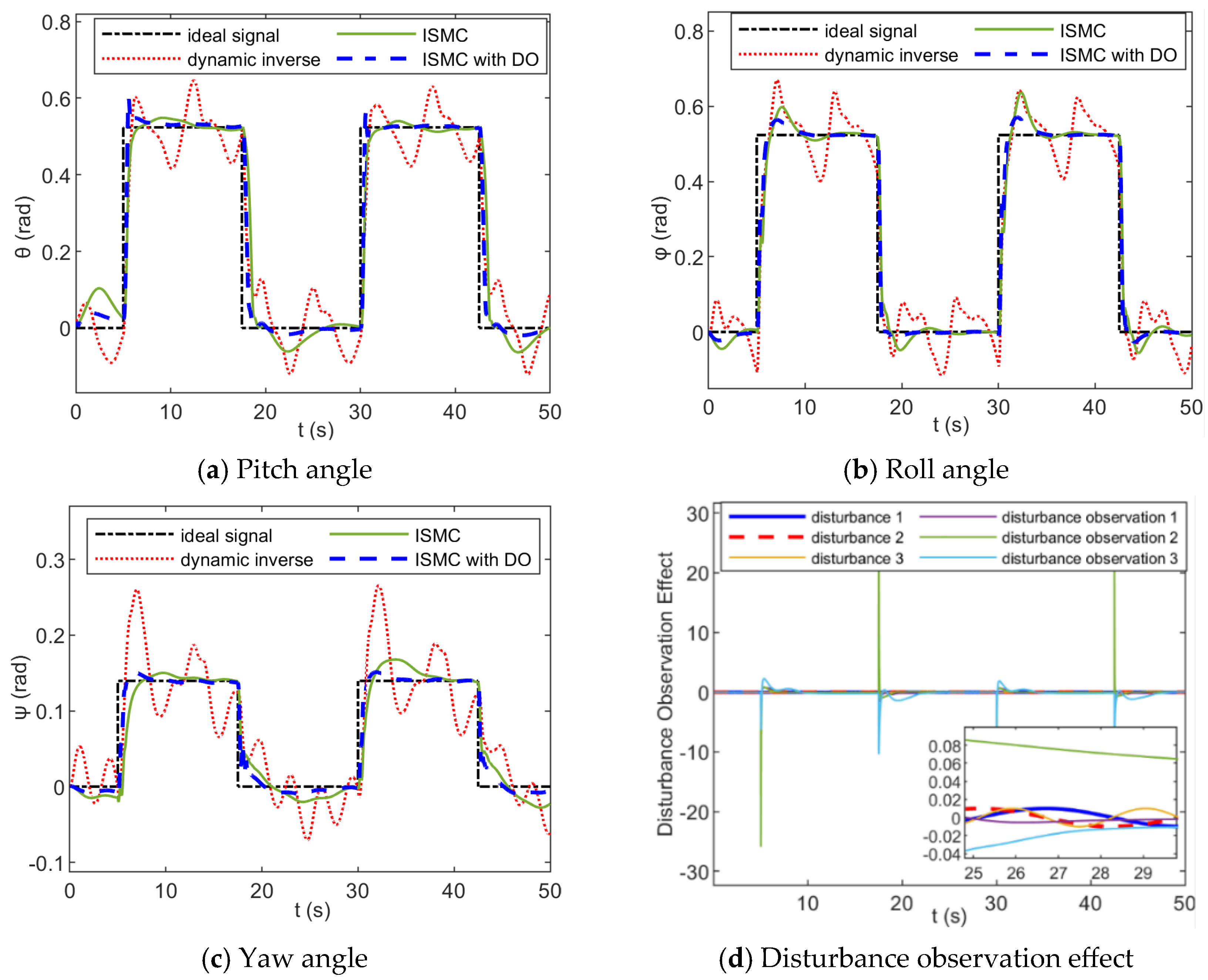
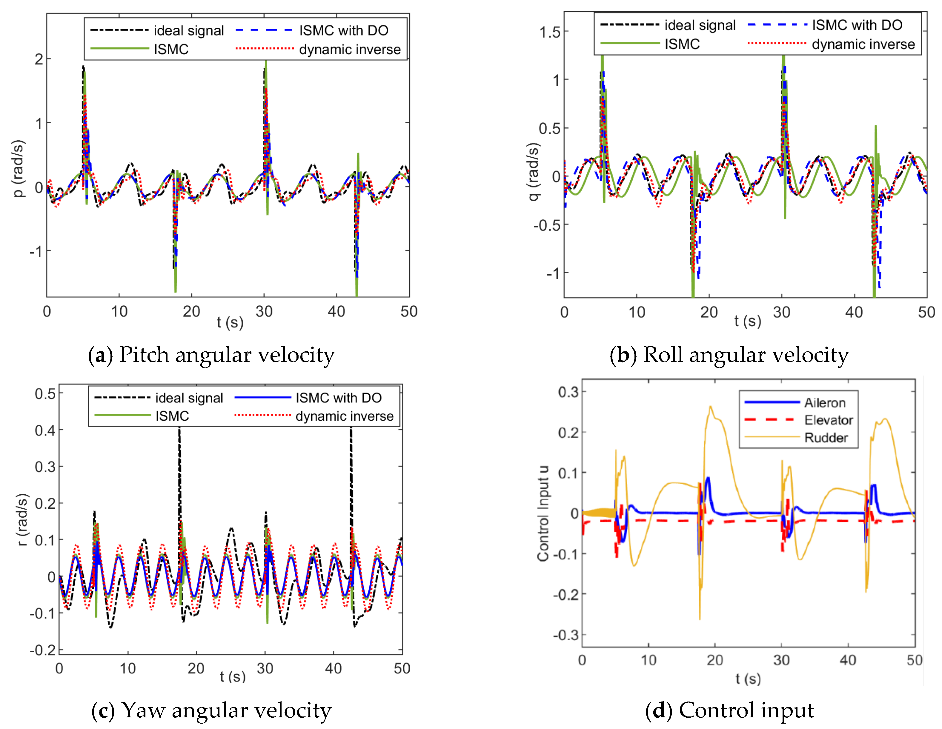
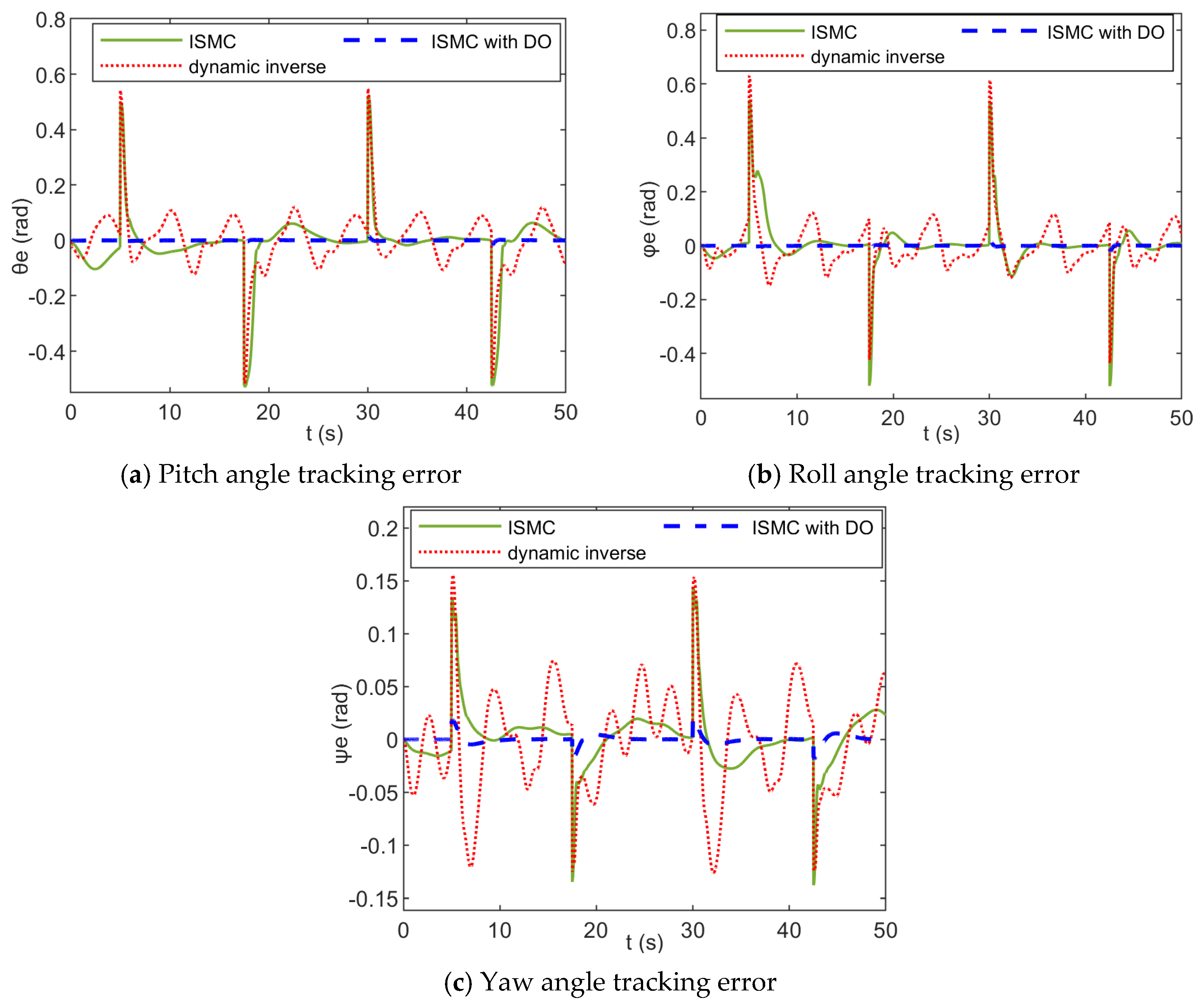
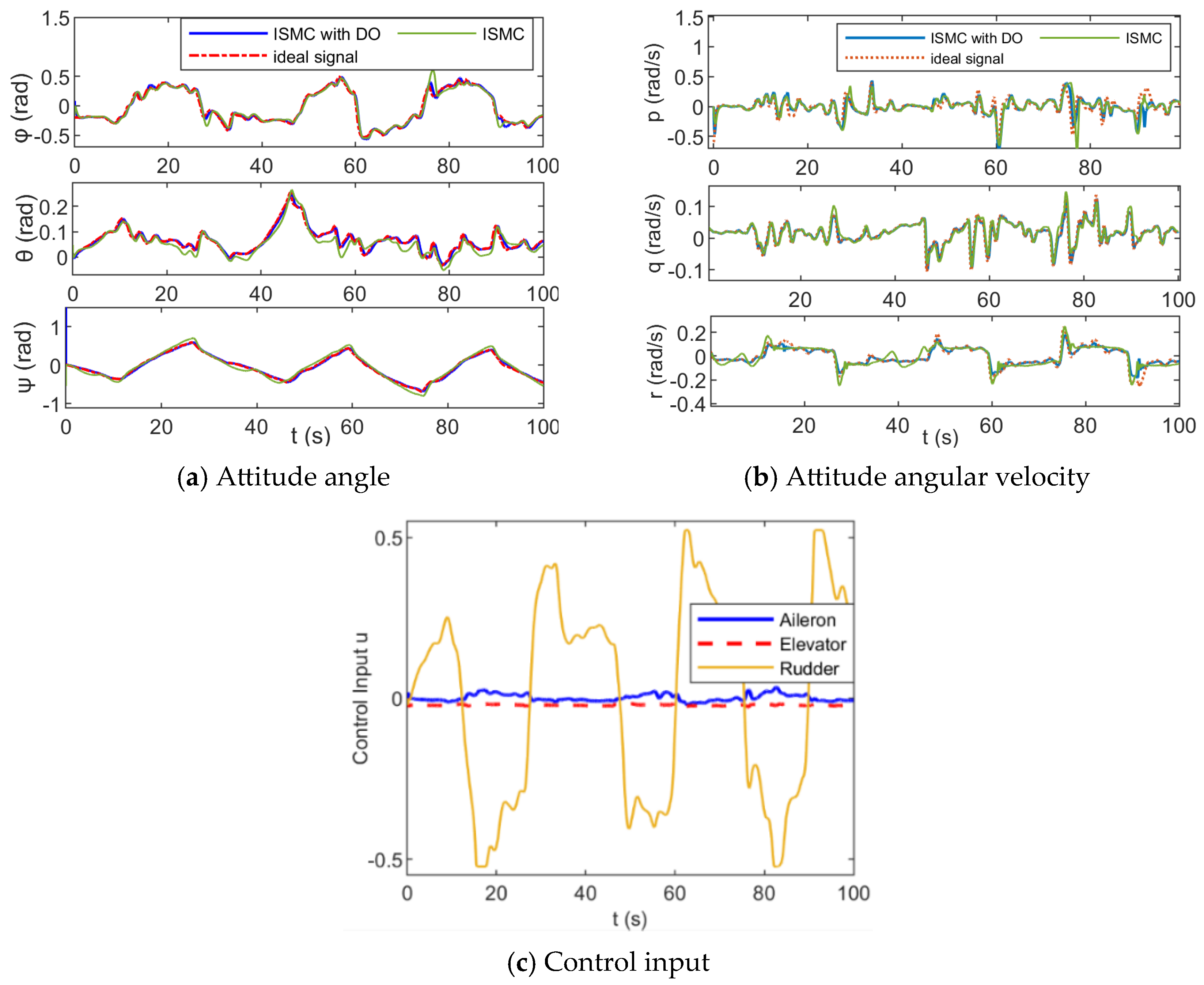
4.1. Anti-Disturbance Attitude Control of Fixed-Wing UAVs Under Sea-Level Low-Altitude Flight

In the realm of engineering, step response serves as a critical tool for assessing the dynamic performance of a control system, offering an opportunity to subject the system to stringent operational conditions through the application of step input. Evaluations of attitude control performance within the body axis coordinate system are conducted by scrutinizing its step response. Figure 3, Figure 4 and Figure 5 depict the influences on attitude tracking when employing dynamic inverse control, ISMC, and ISMC-DO. For these simulations, the initial attitude angles $\eta ={[\begin{array}{ccc}\varphi & \theta & \psi \end{array}]}^T$ and angular velocities $\rho ={[\begin{array}{ccc}{v}_p& v_q& v_r\end{array}]}^T$ are set to zero, and the external disturbances are assumed to be $d={[\begin{array}{ccc}\sin t& \cos t& \sin 2t\end{array}]}^T$.

Figure 3, Figure 4 and Figure 5 reveal a noticeable overshoot in the attitude angles when employing dynamic inverse control, especially when exposed to external disturbances. In such conditions, tracking errors oscillate within $[-0.1,+0.1]$, rendering this approach insufficient for accurate attitude tracking. In contrast, the attitude control strategy based on ISMC-DO excels in rapid tracking performance, even in the face of parameter uncertainties and external disturbances. Each attitude angle manifests minimal overshoot, and the adjustment time falls within a 3 s window. Moreover, the angular velocity closely adheres to the guidelines set by the inner loop instruction. Therefore, the ISMC-DO technique demonstrates superior efficacy in both tracking speed and control accuracy.

While step response serves as an insightful tool for gauging the performance of the controller, real flight conditions often require tracking of a command signal. Therefore, we subjected the dynamic inverse control, ISMC, and ISMC-DO methods to square-wave tracking. In these tests, external disturbances were designated as $d={[\begin{array}{ccc}\sin t& \cos t& \sin 2t\end{array}]}^T$, and the angle tracking instructions ${\eta }_c={[\begin{array}{ccc}{\varphi }_c& {\theta }_c& {\psi }_c\end{array}]}^T$ were characterized as square waves. Specifically, ${\varphi }_c$ and ${\theta }_c$ are square waves featuring an amplitude of π/6 rad, a period of 25 s, a 50% pulse width, and a 5 s phase delay; ${\psi }_c$ follows similar characteristics, but with an amplitude of 2π/45 rad. Figure 6, Figure 7 and Figure 8 illustrate the resulting effects on attitude tracking.

According to the simulation findings, ISMC-DO outperforms both ISMC and dynamic inverse control in terms of tracking error, while exhibiting robustness against disturbances—except in scenarios where angle changes are particularly abrupt. This superiority is attributed to the ability of the ISMC to neutralize parameter uncertainties engendered by fuel consumption, coupled with the capabilities of the DO in estimating wave disturbances. Consequently, this ensures precise attitude tracking for low-altitude UAVs, even when subjected to unpredictable disturbances, thereby augmenting the resistance of the system to such disturbances.

However, Figure 8 indicates instances where the tracking error of ISMC-DO is marginally greater than that of the dynamic inverse method, specifically during abrupt angle changes. Such outcomes arise because the dynamic inverse approach [42] assumes constant model parameters, thus yielding smaller errors. Nevertheless, real-world flight conditions inevitably introduce parameter uncertainties due to fuel consumption. Despite inducing some degree of chattering, ISMC-DO offers a more authentic representation of the attitude control capabilities of the UAV under low-altitude flight conditions.

4.2. Anti-Disturbance Attitude Control of Fixed-Wing UAVs Under Large-Angle Maneuvering

The adoption of the quaternion theory into the ISMC-DO-based control framework effectively mitigates the singularity issues intrinsic to the Euler angle model. Unlike Euler angles, quaternions are devoid of singular points, thus reducing the nonlinearity of the problem. Relying on the amassed maneuver command data—which encompass looping, the split-S, the Pougatcheff cobra maneuver, and the Immelmann turn [42]—we conducted maneuver command tracking experiments using both ISMC and ISMC-DO. The following figures depict the tracking performance in terms of trajectory, attitude angle, and angular velocity during these maneuvers.

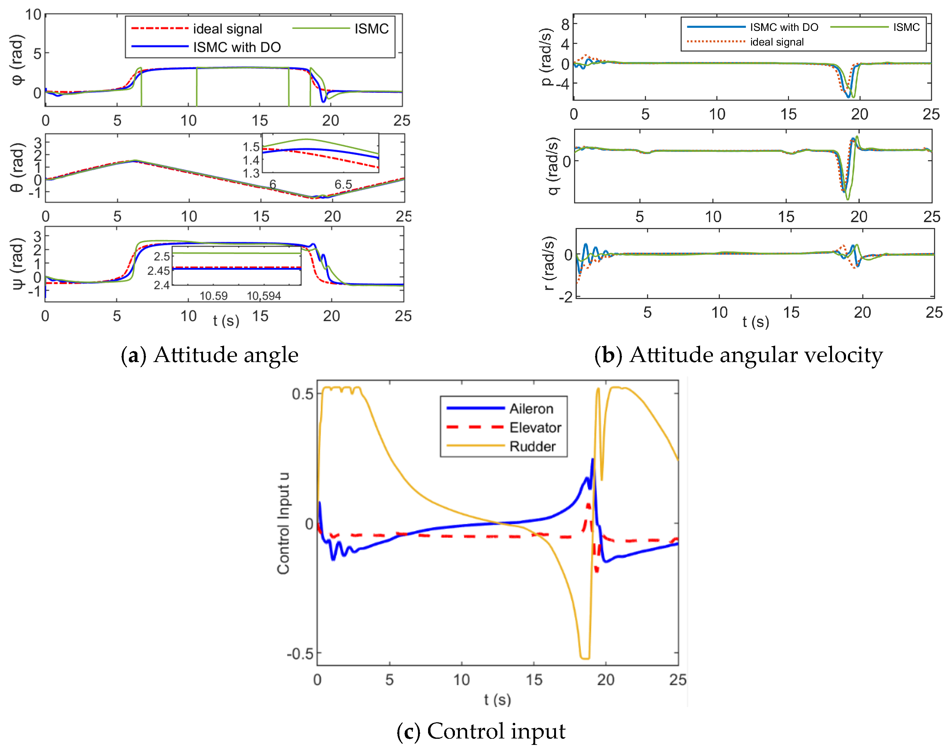
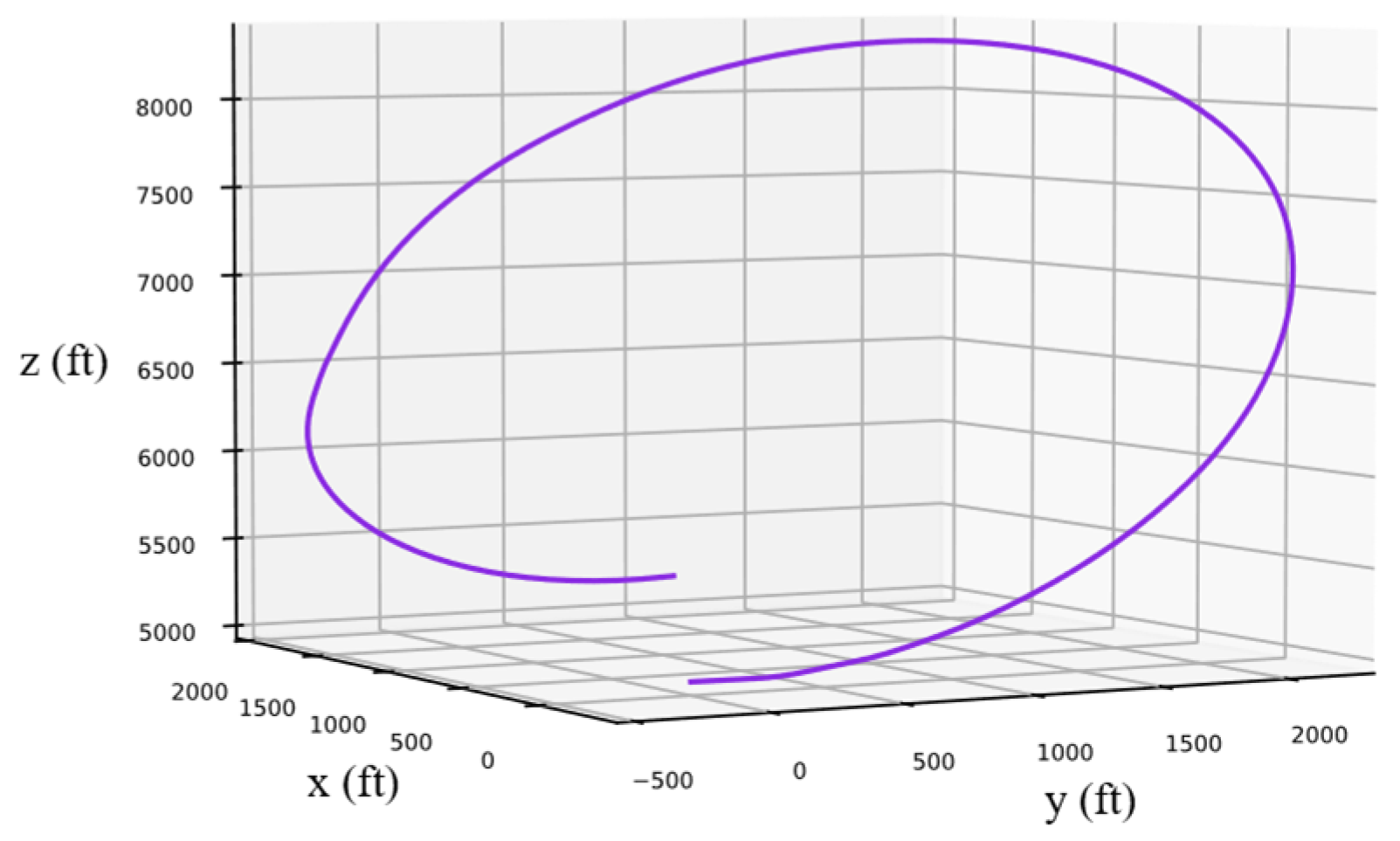
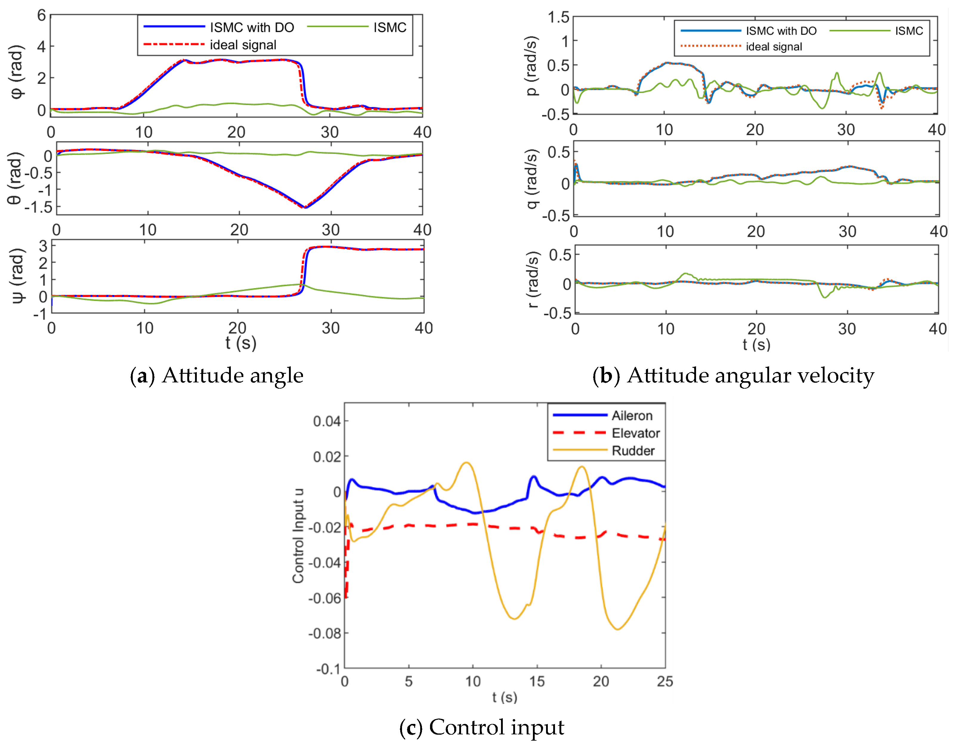
4.2.1. Simulation of Attitude Control of “Looping”

During a “looping” maneuver, the aircraft executes an elliptical path within the vertical plane, undergoing a 360°directional shift. Comprising phases like jumping, inverted flying, and diving, this complex movement is depicted in Figure 9 and Figure 10.

Leveraging a control methodology that amalgamates the quaternion theory with ISMC-DO, the “looping” maneuver is successfully executed. The simulation outcomes substantiate that this methodology enhances tracking performance for both roll and yaw angles, while alleviating singularities. Notably, due to issues related to the conversion between quaternion and Euler angles, special attention is accorded to the yaw angle. Consequently, its overall superposition stands at 2π after 18 s. Throughout the maneuver, the roll and yaw angular velocities remain near zero, while the pitch angle rate remains approximately constant.

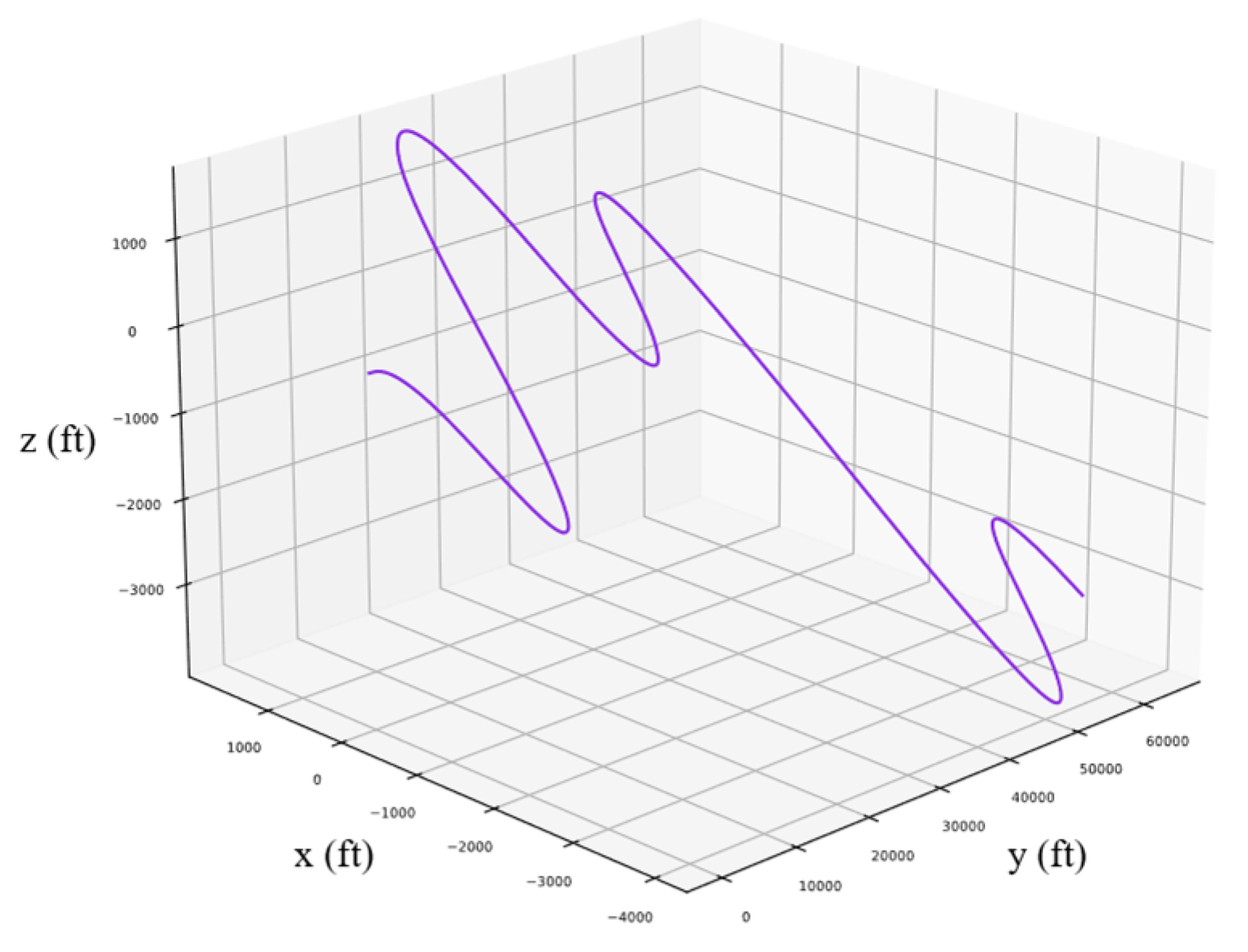
4.2.2. Simulation of Attitude Control of “Split-S”

The “split-S” maneuver is essentially a half-inverted somersault that originates from a roll. This maneuver not only amplifies the velocity of the UAV, but also results in a reduced altitude and a 180° change in course. The resulting simulation data for the “split-S” maneuver are displayed in Figure 11 and Figure 12.

As delineated in these figures, during the “split-S” maneuver, the UAV modifies its roll angle by 180° at a designated roll angular velocity. Subsequently, the aircraft elevates its pitch velocity, transiting from an initial 0° to a −90° position, and then back to 0, while maintaining a constant pitch velocity.

4.2.3. Simulation of Attitude Control of “Pougatcheff Cobra Maneuver”

The “Pougatcheff cobra maneuver” can be conceptualized as an amalgamation of a horizontal turn followed by a set and level flight. When the UAV alters its trajectory, this phase is effectively approximated by a horizontal turn. Subsequently, upon reaching the apex of the main course deviation, the motion of the UAV can be approximated as a set and level flight. Figure 13 and Figure 14 present the simulation results.

As delineated in these figures, the “Pougatcheff cobra maneuver” instigates periodic course adjustments for the UAV through alternating roll angles ranging approximately between 30° and −30. This alternation manifests as a serpentine-like horizontal flight path. Concurrently, the yaw and pitch angles undergo nearly periodic fluctuations. Amidst these complex conditions, the ISMC-DO control system proves its capability to adhere to maneuvering instructions under stringent testing scenarios.

4.2.4. Simulation of Attitude Control of “Immelmann Turn”

Frequently termed a “rising half-roll inversion”, the Immelmann turn consists of a forward somersault initiated from level flight. Upon reaching the zenith of the somersault, the UAV swiftly transitions from an inverted to an upright orientation, subsequently leveling out. This particular maneuver offers tactical advantages, such as rapid altitude gain and a superior position for trailing enemy aircraft. Figure 15 and Figure 16 display the simulation outcomes for this maneuver.

The figures reveal that the pitch angle during the “Immelmann turn” cycles from 0° to 90° and back to 0. Upon completing half of the somersault, the UAV executes a 180° roll at a specified angular rate. Through these simulation assessments, the efficacy of the quaternion-based ISMC-DO attitude control approach for fixed-wing UAVs is substantiated. The results offer considerable insights for the execution of intricate maneuvers, underlining the robustness and applicability of the method.

5. Conclusions

We have introduced an ISMC-DO as a robust solution for anti-disturbance attitude control in fixed-wing UAVs operating at low altitudes. Initially, to mitigate the uncertainties in parameters arising from fuel consumption, a double-closed-loop ISMC system was meticulously designed. Then, a DO was integrated to precisely estimate unexpected ocean wave disturbances, thus improving attitude tracking accuracy during low-altitude flights. It can be rigorously confirmed that the ISMC-DO-based control architecture is asymptotically stable when analyzed through a Lyapunov function. Furthermore, for the purpose of executing large-angle maneuvers, the quaternion theory was employed to bypass the limitations of the Euler angle model. Simulation results robustly demonstrate that, even in the presence of model inaccuracies, external disruptions, and singularities in attitude angles, the ISMC-DO system successfully bolsters the anti-disturbance resilience of the UAV, while maintaining high levels of attitude tracking accuracy. As a future avenue of research, the applicability of the ISMC-DO methodology will be explored for the landing control of shipborne UAVs on surface vessels.

References

1. Wang, X.; Liu, Z.; Cong, Y.; Li, J.; Chen, H. Miniature fixed-wing UAV swarms: Review and outlook. Acta Aeronaut. Astronaut. Sin. 2020, 41, 23732. [Google Scholar] [CrossRef]
2. Wu, Z.; Ni, J.; Qian, W.; Bu, X.; Liu, B. Composite prescribed performance control of small unmanned aerial vehicles using modified nonlinear disturbance observer. ISA Trans. 2021, 116, 30–45. [Google Scholar] [CrossRef] [PubMed]
3. Yang, W.; Shi, Z.; Zhong, Y. Robust adaptive three-dimensional trajectory tracking control scheme design for small fixed-wing UAVs. ISA Trans. 2023, 141, 377–391. [Google Scholar] [CrossRef] [PubMed]
4. Yan, D.; Zhang, W.; Chen, H.; Shi, J. Robust control strategy for multi-UAVs system using MPC combined with Kalman-consensus filter and disturbance observer. ISA Trans. 2023, 135, 35–51. [Google Scholar] [CrossRef]
5. De Marco, A.; D’Onza, P.M.; Manfredi, S. A deep reinforcement learning control approach for high-performance aircraft. Nonlinear Dyn. 2023, 111, 17037–17077. [Google Scholar] [CrossRef]
6. Ren, Z.; Zhang, D.; Tang, S.; Xiong, W.; Yang, S.-H. Cooperative maneuver decision making for multi-UAV air combat based on incomplete information dynamic game. Def. Technol. 2023, 27, 308–317. [Google Scholar] [CrossRef]
7. Nian, X.-H.; Zhou, W.-X.; Li, S.-L.; Wu, H.-Y. 2-D path following for fixed wing UAV using global fast terminal sliding mode control. ISA Trans. 2022, 136, 162–172. [Google Scholar] [CrossRef]
8. Sun, R.; Zhou, Z.; Zhu, X. Flight quality characteristics and observer-based anti-windup finite-time terminal sliding mode attitude control of aileron-free full-wing configuration UAV. Aerosp. Sci. Technol. 2021, 112, 106638. [Google Scholar] [CrossRef]
9. SaiCharanSagar, A.; Vaitheeswaran, S.M.; Shendge, P.D. Uncertainity Estimation Based Approach To Attitude Control of Fixed Wing UAV. IFAC-Pap. 2016, 49, 278–283. [Google Scholar] [CrossRef]
10. Olavo, J.L.G.; Thums, G.D.; Jesus, T.A.; Pimenta, L.C.d.A.; Torres, L.A.B.; Palhares, R.M. Robust Guidance Strategy for Target Circulation by Controlled UAV. IEEE Trans. Aerosp. Electron. Syst. 2018, 54, 1415–1431. [Google Scholar] [CrossRef]
11. Baldi, S.; Sun, D.; Xia, X.; Zhou, G.; Liu, D. ArduPilot-Based Adaptive Autopilot: Architecture and Software-in-the-Loop Experiments. IEEE Trans. Aerosp. Electron. Syst. 2022, 58, 4473–4485. [Google Scholar] [CrossRef]
12. Zhao, D.; Liu, Y.; Wu, X.; Dong, H.; Wang, C.; Tang, J.; Shen, C.; Liu, J. Attitude-Induced error modeling and compensation with GRU networks for the polarization compass during UAV orientation. Measurement 2022, 190, 110734. [Google Scholar] [CrossRef]
13. Mullen, J.; Bailey, S.C.C.; Hoagg, J.B. Filtered dynamic inversion for altitude control of fixed-wing unmanned air vehicles. Aerosp. Sci. Technol. 2016, 54, 241–252. [Google Scholar] [CrossRef]
14. Yu, X.; Yang, J.; Li, S. Finite-time path following control for small-scale fixed-wing UAVs under wind disturbances. J. Frankl. Inst. 2020, 357, 7879–7903. [Google Scholar] [CrossRef]
15. Sufendi; Trilaksono, B.R.; Nasution, S.H.; Purwanto, E.B. Design and implementation of hardware-in-the-loop-simulation for uav using pid control method. In Proceedings of the 2013 3rd International Conference on Instrumentation, Communications, Information Technology and Biomedical Engineering (ICICI-BME), Bandung, Indonesia, 7–8 November 2013; pp. 124–130. [Google Scholar]
16. Azar, A.T.; Serrano, F.E.; Koubaa, A.; Taha, M.A.; Kamal, N.A. Chapter 9-Fast terminal sliding mode controller for high speed and complex maneuvering of unmanned aerial vehicles. In Unmanned Aerial Systems; Koubaa, A., Azar, A.T., Eds.; Academic Press: Cambridge, MA, USA, 2021; pp. 203–230. [Google Scholar]
17. Groves, K.; Sigthorsson, D.; Serrani, A.; Yurkovich, S.; Bolender, M.; Doman, D. Reference command tracking for a linearized model of an air-breathing hypersonic vehicle. In Proceedings of the AIAA Guidance, Navigation, and Control Conference and Exhibit, San Francisco, CA, USA, 15–18 August 2005; p. 6144. [Google Scholar]
18. Bauersfeld, L.; Spannagl, L.; Ducard, G.J.J.; Onder, C.H. MPC Flight Control for a Tilt-Rotor VTOL Aircraft. IEEE Trans. Aerosp. Electron. Syst. 2021, 57, 2395–2409. [Google Scholar] [CrossRef]
19. Guerrero-Sánchez, M.E.; Hernández-González, O.; Valencia-Palomo, G.; López-Estrada, F.R.; Rodríguez-Mata, A.E.; Garrido, J. Filtered Observer-Based IDA-PBC Control for Trajectory Tracking of a Quadrotor. IEEE Access 2021, 9, 114821–114835. [Google Scholar] [CrossRef]
20. Durán-Delfín, J.E.; García-Beltrán, C.D.; Guerrero-Sánchez, M.E.; Valencia-Palomo, G.; Hernández-González, O. Modeling and Passivity-Based Control for a convertible fixed-wing VTOL. Appl. Math. Comput. 2024, 461, 128298. [Google Scholar] [CrossRef]
21. Sartori, D.; Quagliotti, F.; Rutherford, M.J.; Valavanis, K.P. Design and development of a backstepping controller autopilot for fixed-wing UAVs. Aeronaut. J. 2021, 125, 2087–2113. [Google Scholar] [CrossRef]
22. Zhang, R.; Zhang, J.; Yu, H. Review of modeling and control in UAV autonomous maneuvering flight. In Proceedings of the 2018 IEEE International Conference on Mechatronics and Automation (ICMA), Changchun, China, 5–8 August 2018; pp. 1920–1925. [Google Scholar]
23. Lungu, M. Backstepping and dynamic inversion combined controller for auto-landing of fixed wing UAVs. Aerosp. Sci. Technol. 2020, 96, 105526. [Google Scholar] [CrossRef]
24. Wang, X.; Tan, C.P.; Wu, F.; Wang, J. Fault-Tolerant Attitude Control for Rigid Spacecraft Without Angular Velocity Measurements. IEEE Trans. Cybern. 2021, 51, 1216–1229. [Google Scholar] [CrossRef]
25. Reinhardt, D.; Johansen, T.A. Control of Fixed-Wing UAV Attitude and Speed based on Embedded Nonlinear Model Predictive Control. IFAC-Pap. 2021, 54, 91–98. [Google Scholar] [CrossRef]
26. Wang, X.; Tan, C.P. Output Feedback Active Fault Tolerant Control for a 3-DOF Laboratory Helicopter With Sensor Fault. IEEE Trans. Autom. Sci. Eng. 2024, 21, 2689–2700. [Google Scholar] [CrossRef]
27. Zhang, C.; Zhang, G.; Dong, Q. Adaptive dynamic programming-based adaptive-gain sliding mode tracking control for fixed-wing unmanned aerial vehicle with disturbances. Int. J. Robust Nonlinear Control 2023, 33, 1065–1097. [Google Scholar] [CrossRef]
28. He, H.; Duan, H. A multi-strategy pigeon-inspired optimization approach to active disturbance rejection control parameters tuning for vertical take-off and landing fixed-wing UAV. Chin. J. Aeronaut. 2022, 35, 19–30. [Google Scholar] [CrossRef]
29. Castañeda, H.; Salas-Peña, O.S.; León-Morales, J.d. Extended observer based on adaptive second order sliding mode control for a fixed wing UAV. ISA Trans. 2017, 66, 226–232. [Google Scholar] [CrossRef]
30. Hou, Y.; Lv, M.; Liang, X.; Yang, A. Fuzzy adaptive fixed-time fault-tolerant attitude tracking control for tailless flying wing aircrafts. Aerosp. Sci. Technol. 2022, 130, 107950. [Google Scholar] [CrossRef]
31. Wang, X.; Sun, S.; Tao, C.; Xu, B. Neural sliding mode control of low-altitude flying UAV considering wave effect. Comput. Electr. Eng. 2021, 96, 107505. [Google Scholar] [CrossRef]
32. Mahgoub, Y.; El-Badawy, A. Nonlinear disturbance observer-based control of a structural dynamic model of a twin-tailed fighter aircraft. Nonlinear Dyn. 2022, 108, 315–328. [Google Scholar] [CrossRef]
33. Petrlík, M.; Báča, T.; Heřt, D.; Vrba, M.; Krajník, T.; Saska, M. A Robust UAV System for Operations in a Constrained Environment. IEEE Robot. Autom. Lett. 2020, 5, 2169–2176. [Google Scholar] [CrossRef]
34. Wang, Y.; Wang, Y.; Ren, B. Energy Saving Quadrotor Control for Field Inspections. IEEE Trans. Syst. Man Cybern. Syst. 2022, 52, 1768–1777. [Google Scholar] [CrossRef]
35. Liu, X.; Yuan, Z.; Gao, Z.; Zhang, W. Reinforcement Learning-Based Fault-Tolerant Control for Quadrotor UAVs Under Actuator Fault. IEEE Trans. Ind. Inform. 2024, 20, 13926–13935. [Google Scholar] [CrossRef]
36. Huang, Z.; Chen, M.; Shi, P. Disturbance Utilization-Based Tracking Control for the Fixed-Wing UAV With Disturbance Estimation. IEEE Trans. Circuits Syst. I Regul. Pap. 2023, 70, 1337–1349. [Google Scholar] [CrossRef]
37. Xu, L.; Qi, G. Function observer based on model compensation control for a fixed-wing UAV. Aerosp. Sci. Technol. 2024, 152, 109325. [Google Scholar] [CrossRef]
38. Chan, P.T.; Rad, A.B.; Wang, J. Indirect adaptive fuzzy sliding mode control: Part II: Parameter projection and supervisory control. Fuzzy Sets Syst. 2001, 122, 31–43. [Google Scholar] [CrossRef]
39. Chen, W.H. Nonlinear Disturbance Observer Based Dynamic Inversion Control of Missiles. IFAC Proc. Vol. 2001, 34, 463–468. [Google Scholar] [CrossRef]
40. Ariyibi, S.O.; Tekinalp, O. Quaternion-based nonlinear attitude control of quadrotor formations carrying a slung load. Aerosp. Sci. Technol. 2020, 105, 105995. [Google Scholar] [CrossRef]
41. Yao, X.; Lian, Y.; Ju, H.P. Disturbance-observer-based event-triggered control for semi-Markovian jump nonlinear systems. Appl. Math. Comput. 2019, 363, 124597. [Google Scholar] [CrossRef]
42. Cao, S.; Wang, X.; Zhang, R.; Yu, H.; Shen, L. From Demonstration to Flight: Realization of Autonomous Aerobatic Maneuvers for Fast, Miniature Fixed-Wing UAVs. IEEE Robot. Autom. Lett. 2022, 7, 5771–5778. [Google Scholar] [CrossRef]
Figure 2. Attitude control structure diagram based on ISMC-DO method.
Drones 09 00164 g002
Figure 3. Step response test comparison of attitude control angles in body axis coordinate system.
Drones 09 00164 g003
Figure 4. Step response test comparison of attitude control angle tracking errors in body axis coordinate system.
Drones 09 00164 g004
Figure 5. Step response test comparison of attitude control angular velocities in body axis coordinate system.
Drones 09 00164 g005
Figure 6. Attitude angle tracking curve comparison under external disturbances.
Drones 09 00164 g006
Figure 7. Attitude angular velocity tracking curve comparison under external disturbances.
Drones 09 00164 g007
Figure 8. Attitude angle tracking error comparison under external disturbances.
Drones 09 00164 g008
Figure 9. Tracking effect comparison of attitude angle and angular velocity of “looping”.
Drones 09 00164 g009
Figure 10. “Looping” trajectory tracking effect.
Drones 09 00164 g010
Figure 11. Tracking effect comparison of attitude angle and angular velocity of “split-S”.
Drones 09 00164 g011
Figure 12. “Split-S” trajectory tracking effect.
Drones 09 00164 g012
Figure 13. Tracking effect comparison of attitude angle and angular velocity of “Pougatcheff cobra maneuver”.
Drones 09 00164 g013
Figure 14. “Pougatcheff cobra maneuver” trajectory tracking effect.
Drones 09 00164 g014
Figure 15. Tracking effect comparison of attitude angle and angular velocity of “Immelmann turn”.
Drones 09 00164 g015
Figure 16. “Immelmann turn” trajectory tracking effect.
Drones 09 00164 g016