Efficient Coverage Path Planning for a Drone in an Urban Environment

Abstract

Multirotor drones play an increasingly significant role in smart cities and are among the most widely discussed emerging technologies. They are expected to support various applications such as package delivery, data collection, traffic policing, surveillance, and medicine. As part of their services, future drones should be able to solve the last-mile challenge and land safely in urban areas. This paper addresses the path planning task for an autonomous drone searching for a landing place in an urban environment. Our algorithm uses a novel multi-resolution probabilistic approach in which visual information is collected by the drone at decreasing altitudes. As part of the exploration task, we present the Global Path Planning (GPP) problem, which uses probabilistic information and the camera’s field of view to plan safe trajectories that will maximize the search success by covering areas with high potential for proper landing while avoiding no-fly zones and complying with time constraints. The GPP problem is formulated as a minimization problem and then is shown to be NP-hard. As a baseline, we develop an approximation algorithm based on an exhaustive search, and then we devise a more complex yet efficient heuristic algorithm to solve the problem. Finally, we evaluate the algorithms’ performance using simulation experiments. Simulation results obtained from various scenarios show that the proposed heuristic algorithm significantly reduces computation time while keeping coverage performance close to the baseline. To the best of our knowledge, this is the first work referring to a multi-resolution approach to such search missions; further, in particular, the GPP problem has not been addressed previously.

1. Introduction

Unmanned aerial vehicles, sometimes generically called drones, are becoming increasingly popular to provide mobility solutions for congested smart cities [1,2]. Equipped with a wide range of sensors and real-time processing capabilities, drones combine the key principles of technological modernity: data processing, networking, autonomy, and mobility. In smart city environments, drones are called to play a major role in a variety of applications, including package delivery [3,4], data collection [5], traffic policing [6], surveillance [7], Search and Rescue (SAR) operations [8,9,10], and even as transportation devices [11]. The integration of drones into densely populated areas presents many challenges due to safety, security, and privacy considerations. This is especially true when considering autonomous operations with little or no human intervention.

To fulfill their intended purposes, drones must be provided with the ability to explore complex urban environments and search for mission-dependent targets. Motivated by this fact, [12] recently considered a multi-resolution probabilistic approach for searching for a landing site in an urban environment by maintaining a probability map quantifying the probability of different areas being suitable for landing. Note that in that paper, as well as in the current one, "multi-resolution” refers to the fact that information is gathered from different altitudes, giving increased spatial resolution when flying at lower altitudes. This is not to be confused with other usages of multiple-resolution, such as image processing tools (e.g., a pyramid parametrization) or employing a sequence of images as in super-resolution. These probabilities are updated based on images taken from a downward-looking camera and by re-visiting certain areas from different viewpoints. In order to do this efficiently, a trajectory planning scheme is required that selects which areas should be re-visited and then computes an efficient and safe trajectory.

In this work, we address the trajectory planning problem outlined above. Following [13], we propose a solution for the Global Path Planning (GPP) problem that aims to plan safe trajectories to explore an area at a constant altitude. Due to time and energy constraints, the trajectories are necessarily limited in length and must cover areas with a high probability of being appropriate for landing.

The remainder of this paper is organized as follows: Section 2 reviews existing work regarding well-known coverage path planning algorithms and related computational geometry problems. The formulation of the GPP problem is provided in Section 3. Section 4 presents a baseline algorithm for the GPP problem based on an exhaustive search. Section 5 introduces SST—an efficient heuristic algorithm for the GPP problem. Performance results are reported in Section 6, and Section 7 concludes the paper.

2. Related Work

The GPP problem studied in this work is related to a wide range of studies in the literature spread across several fields, from computational geometry problems to coverage and optimal trajectory planning. Indeed, the problem can be considered a variation of area coverage, initially formulated by [14] and extensively studied since then. Coverage Path Planning (CPP) can be formulated as follows: given a specified region in 2D or 3D, plan a trajectory for one or multiple robots such that every point in the region is visited while avoiding obstacles. Applications of the CPP problem are numerous and include part painting in the automobile industry, guaranteeing full floor cleaning or grass cutting, and finding people in distress in emergency areas. The survey provided by [15] provides a good introduction and pointers to the literature.

In a typical CPP formulation, the area to be visited is divided into two sub-regions: the Area of Interest (AOI) and obstacles. The AOI is sometimes divided into smaller cells, and each cell may have a deterministic or probabilistic value attached to it. Probabilistic values may help establish an order in which the cells are to be visited and are commonly used when performing search tasks. For instance, Refs. [9] and [16] calculate a discrete path for a drone by using probability maps where each cell represents the potential risk/occupancy degree. In particular, [16] develops a greedy algorithm that uses clustering to accumulate maximum probabilities and is limited by the maximum allowed length.

Another extensive survey [17] specifically considers the coverage problem using drones. Although the land and air versions of the problem are strongly related, planning a coverage path for a drone includes some additional features, including the limited endurance of the platform, its maneuverability limitations, restricted payload, obstacles that may cause occlusions, and other similar issues. The survey revises different CPP approaches, from simple geometric flight patterns for non-complex AOI to more complex grid-based solutions considering full and partial information about the AOI.

The use of drones for coverage tasks requires considering their mounted camera properties, which can only capture points with a cone-shaped Field of View (FOV). The FOV of the camera can be further reduced by obstacles like buildings and walls. To achieve complete coverage of the AOI, each point must be mapped onto the image plane at least once in a complete trajectory. This was considered, for instance, in [7,18], which introduce two-step trajectory planning algorithms for coverage missions of geometrically complex environments that consider camera sensing constraints. First, they find a set of waypoints from which the AOI can be covered fully; then, they plan a smooth trajectory along these waypoints such that the completion time is minimal. In [19], a flight path planning algorithm is proposed to find collision-free, minimum-length paths for drones’ coverage missions. The authors use a footprints’ sweeps fitting method to address this problem, considering the camera footprint as a coverage unit.

In drone coverage missions, the AOI is sometimes partitioned using a grid where the camera footprint determines the size of each cell [20]. As a result, the drone can observe an entire cell when located at its geometrical center, and the area is said to be fully covered when it visits the centers of all cells.

The GPP problem discussed in this paper consists of finding a safe path covering an AOI while meeting a time constraint—i.e., the path length is limited. As a result, it is not possible to scan the entire AOI but to choose which sub-areas have a high priority for scanning. In the case described in [5,21], a drone needs to visit several spatially distributed Points of Interest (POIs) to maximize the information collected subject to energy constraints. Similarly, [8] suggests an efficient localization solution for SAR missions. For this case, given a map indicating the importance level of each area, the planning algorithm should determine strategic waypoints at which the UAV hovers and collects data while an efficient trajectory composed of all waypoints is generated using a solution to the Traveling Salesman Problem (TSP).

The tasks of selecting a set of waypoints and optimal routing between these points are dealt with in familiar computational geometry problems. The art gallery problem [22] considers a polygonal gallery where a minimum number of guards are to be positioned such that at least one guard can see every point in the gallery; the watchman route problem [23] seeks the shortest route a watchman should take so that every point in a given space can be seen from at least one point along the route; the orienteering problem [24] aims to construct a path through a set of nodes that maximizes the total score and does not exceed a given budget; and probably the most famous one, the TSP [25]—all these problems have been proven to be NP-hard and are often solved by approximation algorithms.

One heuristic method commonly used for solving the optimization problems mentioned above is local search [26]. In a typical local search algorithm, an initial solution is first constructed, for instance, by a greedy algorithm. Then, in an iterative manner, the initial solution is modified by local operations, with a slight improvement in each iteration. Ref. [27] presents a random mixed local search method for finding an optimal solution for the Open-Loop Traveling Salesman Problem (OLTSP). Starting with some initial trajectory, the algorithm improves this method (in terms of length) by mixing in local search operators (NodeSwap, 2opt, LinkSwap).

Most of the approaches mentioned above use offline solutions computed before the mission is actually executed. Therefore, computing time is of secondary importance and is usually not a measure of the algorithm’s quality. In the case considered in this study, computation time is a significant factor. During the mission of autonomous landing, it is necessary to find a trajectory at decreasing altitudes—i.e., the GPP problem is to be solved several times in a short period. Therefore, in addition to the requirement of finding a near-optimal solution, we aim to develop an algorithm that is also efficient in terms of computation time.

3. System Model and Problem Definition

In this section, the system model and the GPP problem are introduced. The GPP problem is then formulated as an optimization problem and shown to be NP-hard.

3.1. System Model

Consider the problem of finding a landing site for a drone in an urban region $\mathcal{A}$. The region $\mathcal{A}$ is assumed to be a plane partially occupied by structures, including buildings, traffic lights, billboards, vegetation, and similar obstacles typical of built environments. The drone, equipped with a downward-looking camera, explores the region $\mathcal{A}$ by following a trajectory that lies on the plane ${\pi }^h$ parallel to $\mathcal{A}$ at a constant altitude h. The region ${\pi }^h$ is divided into two complementary sub-regions ${\pi }^h={\pi }_f^h\cup {\pi }_o^h$, where the former is the area where the drone is permitted to fly safely and securely while the latter is a no-fly zone (NFZ), i.e., an area where the drone cannot fly due to obstacles or regulations.

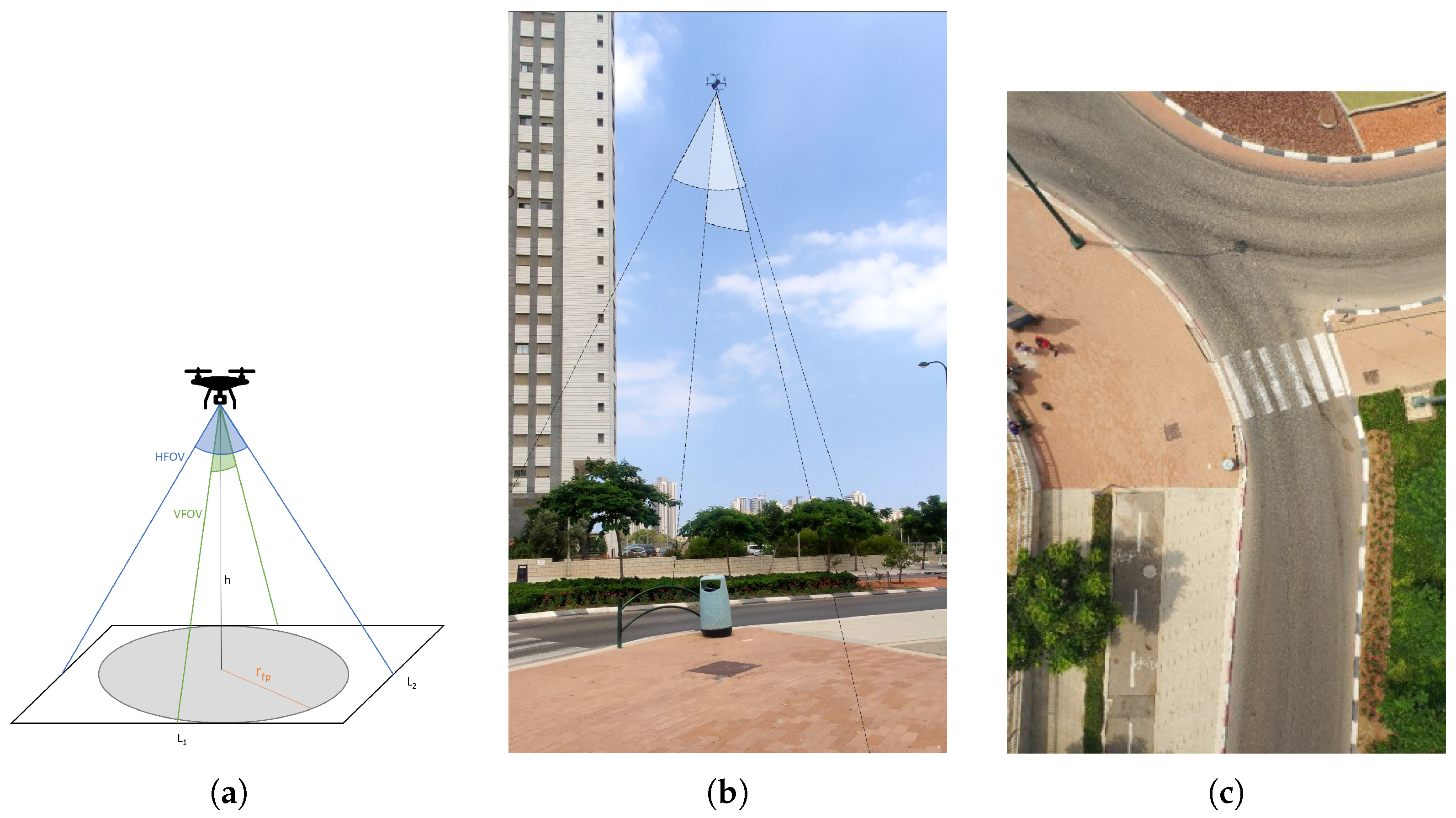
Throughout the flight, subsets of $\mathcal{A}$ are projected onto the camera image plane. Let ${\mathcal{I}}_k=\mathcal{I}\left(w_k\right)$ and ${\mathcal{F}}_k\subset \mathcal{A}$ denote the image taken by the camera at the waypoint $w_k\in {\pi }_f^h$ and the corresponding footprint on $\mathcal{A}$. The image taken at waypoint $w_k$ will be such that its center lies at the intersection between the camera’s line of sight and the image plane. As illustrated in Figure 1, the size of the camera footprint ${\mathcal{F}}_k$ is a function of the drone altitude and the FOV of the camera. The dimensions of the footprint can be calculated using the following:

$$\begin{array}{cc}\hfill L_1& =2·h·tan\left(\frac{HFOV}{2}\right)\hfill \\ \hfill L_2& =2·h·tan\left(\frac{VFOV}{2}\right)\hfill \\ \hfill r_{fp}& =min(L_1,L_2)/2\hfill \end{array}$$

(1)

In order to guarantee a safe landing place, $\mathcal{A}$ can be discretized into $M\times N$ identical grid cells $c_{mn}$ such that $\bigcup c_{mn}=\mathcal{A}$. As shown in Figure 2, the cell dimensions are derived from the size of the body and propellers of the drone together with the flying conditions (e.g., wind). This partition is in line with discrete search theory (see, e.g., [28]) but with a different motivation.

Following this, a probability $p_{mn}$, with $0\le p_{mn}\le 1$, is attached to each cell $c_{mn}$, resulting in a probability map modeling the likelihood that each cell is suitable for landing. Then, the idea is to re-explore cells with a relatively high probability and update their values. As the level of certainty increases, the probabilities are likely to approach ‘1’ or ‘0’ until one or more probabilities exceed a certain threshold, making it possible to determine that the corresponding cell is suitable for landing. See [12] for a detailed discussion.

3.2. Initialization

The information available prior to the beginning of the landing mission is a Digital Surface Model (DSM) of the explored area, from which the locations of the obstacles at any height can be extracted. The obstacles are approximated by polygons, and their vertices are given in the world coordinate system.

According to the DSM, an initial probability map is built. As no additional information is available, the values in this probability map are ‘0’ for cells that belong to obstacles and ‘0.5’ otherwise, meaning that, at first, all cells in the free area are equal candidates for a landing site.

3.3. Global Path Planning Problem

The objective of the GPP problem is to find a safe trajectory that begins at an initial position $w_0$ and covers areas with a high potential of being a proper landing site. As the drone has limited energy and performs the trajectory in an urban area, the planned trajectory must comply with a time-of-flight constraint and avoid NFZ.

For a given image footprint ${\mathcal{F}}_k$, let the set of pairs of indices $J_k$ be

$$J_k=\{(m,n)\mathrm{s}.\mathrm{t}.c_{mn}\subset {\mathcal{F}}_k\}$$

(2)

Also, given $0<\underline{p}\le 1$, let $\mathrm{\Gamma }\left(\underline{p}\right)$ be the following set of pairs of indices:

$$\mathrm{\Gamma }\left(\underline{p}\right)=\{(m,n)\mathrm{s}.\mathrm{t}.p_{mn}\ge \underline{p}\}$$

(3)

With this definition, we can treat $\underline{p}$ as a threshold value that separates the cells of interest from the remaining cells.

Definition 1.

The set of waypoints $W^h=\{w_0,w_1,...,w_k\}$, $w_i\in {\pi }^h$ is said to be a $\underline{p}$ -Coverage (note that this definition is different from the one in [29] for k-coverage—the latter ensures each cell is covered by at least k covers) at altitude h if for all $(m,n)\in \mathrm{\Gamma }\left(\underline{p}\right)$ there exists at least one $w_i$ such that $c_{mn}\subset {\mathcal{F}}_i$.

In general, a footprint contains numerous cells; therefore, $\underline{p}$-Coverage sets are far from unique, and two different ones may have a different number of elements.

Definition 2.

A trajectory passing through $W^h$ is a continuous map $T:[t_0,t_{end}]\to {\pi }^h$ such that $T\left(0\right)=w_0$ and there exists a set of time instants ${\left\{t_i\right\}}_{i=1,·,k}$ such that $T\left(t_i\right)=w_i,\forall w_i\in W^h$. The trajectory is said to be $\underline{p}$-covering if $W^h$ is a $\underline{p}$-Coverage.

In the following, T will simply be referred to as a trajectory, since $W^h$ will be clear from the context. Note that the set of time instants in the definition is, in general, not ordered—namely, $i<j\Rightarrow t_i<t_j$.

Definition 3.

A cell $c_{mn}$ is said to be visited by a trajectory T if $c_{mn}\subset {\mathcal{F}}_k$ for some k.

Definition 4.

A trajectory is said to be safe if $T\left(t\right)\in {\pi }_f^h$ for all $t\in [t_0,t_{end}]$.

As a standard when introducing new planning algorithms, no dynamic constraints are placed in the definition of feasible trajectories.

3.4. Exact Formulation

Define a cost function $\tau (·)$ over all safe trajectories T. The cost function measures a property of the trajectory that one would like to control. For definiteness, a total traveling time constraint is assumed here; hence, let ${\tau }_{max}$ be the maximal time-of-flight allowed for the trajectory.

With these definitions, the GPP can be translated into the problem of finding the minimum value of p such that there exists a safe, p-covering trajectory for which $\tau \left(T\right)=t_{end}-t_0\le {\tau }_{max}$:

$$\begin{array}{cc}\hfill min& p\\ \hfill \mathrm{s}.\mathrm{t}. \mathrm{f}\mathrm{o}\mathrm{r} \mathrm{s}\mathrm{o}\mathrm{m}\mathrm{e} T& \\ & \tau \left(T\right)\le {\tau }_{max}\\ & \forall (m,n)\in \mathrm{\Gamma }\left(p\right):c_{m,n}\subset \mathcal{F}\left(T\right)\\ & T\in {\pi }_f\end{array}$$

(4)

The first constraint guarantees that the desired cost is not violated. For a given p, the second constraint requires T to be p-covering. Finally, the third constraint promises the safeness of T.

Notice that for $\underline{p}\approx 1$, the $\underline{p}$-coverage set $W^h$ will be relatively small, and hence, one would expect to meet the upper bound ${\tau }_{max}$ of the cost function. As $\underline{p}$ gets smaller, the number of cells to be visited increases, and so eventually, the upper bound might not be met by any feasible trajectory. The problem, therefore, captures the desirable property of visiting as many cells as possible while concentrating on the higher probability ones.

Theorem 1.

GPP is an NP-hard problem.

Proof. 

To prove the NP-hardness of the problem, we use a known NP-hard problem, the Orienteering Problem (OP) [30], and reduce it to the GPP problem in a polynomial time. The OP is formulated as follows. Given n nodes in the Euclidean plane $[v_1,..,v_i,..,v_n]$, each with a score $s\left(i\right)\ge 0$, find a route of maximum score through these nodes beginning at $v_1$ and ending at $v_n$ of length no greater than $T_{MAX}$.

Consider an instance $\mathcal{P}$ of the OP. We reduce it to a GPP problem by the following operations.

• Place the nodes on a grid such that a single cell does not contain more than one node.
• Convert the scores to probabilities by normalizing them.
• Generate a probability map $\mathcal{M}$ out of the grid by assigning the score values to cells containing nodes and 0 otherwise.
• To ensure the selection of $v_N$ and its position at the end of the path, set $p\left(v_N\right)=\infty$ and $dist(v_N,v_i)=\infty \forall i$.
• Set the required initial waypoint as $v_1$.

Define ${\mathcal{P}}^{\prime }$ as a GPP problem with a probability map $\mathcal{M}$, initial position $v_1$, and time constraint $T_{MAX}$. With the assumption of a single-cell size footprint, the minimization of p in ${\mathcal{P}}^{\prime }$ is equivalent to the maximization of the total score in $\mathcal{P}$. □

The optimization problem considered above provides a mathematical formulation of the GPP problem. In Section 4 and Section 5, two alternative approaches for solving the GPP problem that trade the simplicity of exhaustive search with a more complex and efficient algorithm will be discussed.

4. Baseline Algorithm

As GPP is a new problem, we have first developed a solution based on an exhaustive search to serve as a baseline. A naive approach for finding the optimal probability threshold $\underline{p}$ for the GPP problem presented in Equation (4) is to list all possible candidates for the solution and check whether each meets the problem’s requirements. This approach results in a factorial algorithm that is, in principle, computationally infeasible for large problems.

As stated before, the value of $\underline{p}$ and the size of the $\underline{p}$-coverage set $W_h$ are inversely proportional. For instance, assume a specific probability threshold $\underline{p}=p_0$ and define the corresponding $p_0$-covering trajectory $T_{p_0}$. In case $T_{p_0}$ violates the cost constraint, then the minimum $\underline{p}$ cannot be lower than $p_0$. Alternatively, if $T_{p_0}$ complies with the constraints, it is certain that the minimum $\underline{p}$ is lower than or equal to $p_0$. Referring to this behavior, a binary search is appropriate for finding the optimal solution.

The Exhaustive Search (ES) algorithm, initially developed, iteratively searches for the minimum probability threshold for which the constraints are met. In each iteration, $\underline{p}$ is fixed, and a corresponding $\underline{p}$-covering trajectory is found. Then, $\underline{p}$ is updated according to whether the found trajectory complies with the constraints until convergence. A detailed description is provided in Algorithm 1.

The inputs to the algorithm are a probability map and obstacle locations corresponding to the region $\mathcal{A}$ at flight altitude h, the required first waypoint, and mission constraints. The output of the algorithm is a trajectory covering a sub-area of $\mathcal{A}$ at a constant altitude that avoids obstacles and meets the time constraints of the mission.

First, a visibility graph [31] is built based on the known obstacle locations. The visibility graph allows for finding collision-free optimal paths between points in the free area ${\pi }_f$. It is used as an auxiliary graph at a later stage when it is desirable to present the connectivity between waypoints. The visibility graph can be built efficiently using, e.g., the Plane Sweep algorithm in [32].

To determine the search boundaries, two variables $min$ and $max$ are initialized with the minimum and the maximum probabilities found in $\mathcal{P}$. The iterative part begins with calculating the threshold $\underline{p}$ as the middle of the search boundaries. Considering the probability map, obstacle locations, and the required first waypoint, a corresponding trajectory $T_{\underline{p}}$ is then found. Starting at $w_0$, the planned trajectory is $\underline{p}$-covering and safe. In case $\tau \left(T_{\underline{p}}\right)\le {\tau }_{max}$, $T_{\underline{p}}\to T$ since it meets all the constraints and corresponds to the minimal threshold found so far. Finally, the search range is narrowed according to the previous comparison: the upper boundary $max$ is reduced to $\underline{p}$ in case the constraints are met, or the lower boundary $min$ is enlarged to $\underline{p}$ if the opposite is true. The search continues until the search interval, i.e., the difference between $max$ and $min$, is less than some $ϵ$.

Algorithm 1: Exhaustive Search

Input: Probability map $\mathcal{P}$, obstacle locations $\mathcal{O}$, first waypoint $w_0$, mission constraints ${\tau }_{max}$ Output:Trajectory T 1: $\mathcal{VG}$ = buildVisibilityGraph($\mathcal{O}$) 2: $min,max\leftarrow$ min_prob($\mathcal{P}$), max_prob($\mathcal{P}$) initialization 3: $diff\leftarrow max-min$ 4: while diff $\ge \epsilon$ do 5:    $\underline{p}\leftarrow$ updateThreshold ($min,max$) 6:    $T_{\underline{p}}\leftarrow$ planTrajectory($\mathcal{P}$, $\mathcal{VG}$, $w_0$, $\underline{p}$) 7:    if $\tau \left(T_{\underline{p}}\right)\le {\tau }_{max}$ then 8:      $T\leftarrow T_{\underline{p}}$ 9:      $max\leftarrow \underline{p}$ {continue the search in the lower half of the range} 10:   else 11:      $min\leftarrow \underline{p}$ {continue the search in the upper half of the range} 12:   end if 13:   $diff\leftarrow max-min$ 14: end while 15: return T

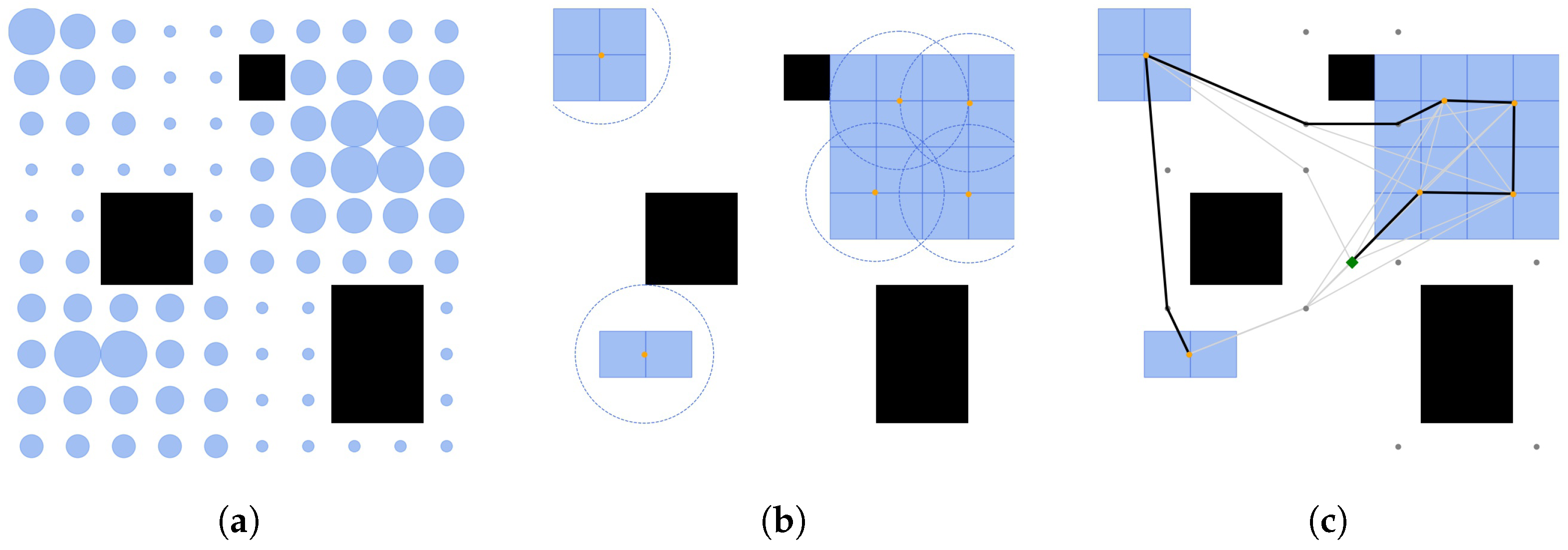
Inspired by [7,8], the process of planning a $\underline{p}$-covering trajectory presented in Algorithm 2 consists of two main parts: waypoint selection and efficient waypoint arrangement. See Figure 3 for a graphical representation. For a given threshold $\underline{p}$, the POIs are described by the set $\mathrm{\Gamma }\left(\underline{p}\right)$. As Equation (2) states, multiple cells are included in the camera footprint when passing through a single waypoint. It is then possible to find a minimum set of strategic waypoints $W^h$, which is $\underline{p}$-covering and guarantees complete and effective coverage of all the POIs. For this purpose, the POIs are clustered such that the size of each cluster does not exceed the camera footprint size. The set $W^h$ is then built by collecting the centers of the clusters so that visiting all $w_k\in W^h$ guarantees $\underline{p}$-coverage. Among the different clustering methods examined, the single-pass algorithm described in [33] proved to be the fastest.

Algorithm 2: planTrajectory

Input: Probability map $\mathcal{P}$, visibility graph $\mathcal{VG}$, first waypoint $w_0$, threshold $\underline{p}$ Output: Trajectory $T\underline{p}$ 1: $POI\leftarrow$ applyThreshold($\mathcal{P}$, $\underline{p}$) 2: $W^h\leftarrow$ClusterPOI($POI$) 3: $W^h$.add($w_0$) 4: $G\leftarrow$buildeGraph($W^h,\mathcal{VG}$) 5: $T_{\underline{p}}\leftarrow$ solveOLTSP(G, I, R) 6: return  $T\underline{p}$

To construct an efficient path that visits all the waypoints, a complete graph G with vertices $W^h$ is built, with the shortest path lengths as its weights. The visibility graph guarantees that the shortest path between each pair of waypoints is collision-free. Based on the complete graph, the visiting order is determined by solving an OLTSP in which the goal is to find the shortest path that visits each waypoint exactly once without returning to the starting position. In particular, the near-optimal algorithm presented in [27] is used with the nearest-neighbor (NN) algorithm [25] as an initialization heuristic. The algorithm is based on local-search operations with two input parameters: the number of iterations I and the number of repetitions R.

The resulting algorithm generates a trajectory that complies with the entire set of constraints and corresponds to the smallest feasible probability threshold.

5. SST—An Efficient Heuristic Algorithm for the GPP Problem

The ES algorithm is memory-less in the sense that it finds a trajectory each time it is called without taking advantage of the fact that the planned trajectories for different altitudes are not entirely uncorrelated. As a result, time-consuming operations are performed repeatedly, resulting in long computation times. This section presents a heuristic algorithm that exploits the mission properties to reduce the computation times while maintaining good performance.

5.1. Overview

Together with being safe and complying with time constraints, the planned trajectory has to maximize the relevant information collected while following that information, allowing better decision-making regarding which landing spot to select. Since any point in the free area ${\pi }_f$ is an appropriate candidate for a trajectory waypoint, selecting a subset of waypoints that maximizes the information among infinitely many possibilities is a great challenge.

To tackle this problem, a pre-processing stage has been added with the aim of finding a finite, narrow set of candidate waypoints $\mathcal{V}$ that will serve the task of trajectory planning throughout the entire mission. Considering this set of candidate waypoints, the planning stage includes three main steps: Score–Select–Traverse (SST).

• Score—Assign each candidate waypoint a score that represents some measure of its corresponding footprint.
• Select—Select a subset of waypoints to form the trajectory.
• Traverse—Determine the visiting order to minimize travel time.

The detailed algorithms for the pre-processing and planning stages are presented in Algorithms 3 and 4, respectively, and further discussed in the following sections.

Algorithm 3: SST—Pre-Processing

Input: A preliminary probability map $\mathcal{P}$, the minimum flying altitude $h_{min}$, obstacle locations in $h_{min}$${\mathcal{O}}_{h_{min}}$ Output: A set of candidate waypoints $\mathcal{V}$, a visibility graph $\mathcal{VG}$ 1: $POI\leftarrow$ extractPOI($\mathcal{P},{\mathcal{O}}_{h_{min}}$) 2: $bandwidth\leftarrow$ calcFootprintSize($h_{min}$) 3: $\mathcal{V}\leftarrow$ ClusterPOI($POI,bandwidth$) 4: $\mathcal{VG}\leftarrow$ PlaneSweep(${\mathcal{O}}_{h_{min}}$) 5: return $\mathcal{V},\mathcal{VG}$

Algorithm 4: SST—Planning

Input: A probability map $\mathcal{P}$, first waypoint $w_0$, mission constraints ${\tau }_{max}$, visibility graph $\mathcal{VG}$ Output: A trajectory T 1: ${\mathcal{G}}^h\leftarrow$ scoreAndSelect($\mathcal{P},w_0,{\tau }_{max},\mathcal{VG}$) 2: $visit\_order\leftarrow$ solveOLTSP(${\mathcal{G}}^h$, I, R) 3: $T\leftarrow$ post_processing($visit\_order$) 4: return T

5.2. Candidate Waypoint Set—$\mathcal{V}$

As part of the planning process (SST), the second step is to select the set of waypoints ${\mathcal{W}}^h\subset \mathcal{V}$ that will form the trajectory in order to ensure that it visits high-probability areas. In the absence of any preliminary operations, the search space is very large since any point included in the map boundaries and within the free space is valid.

In order to reduce computation times for the planning stage, the search space is narrowed down to a set of candidate waypoints $\mathcal{V}$ that are found in a pre-processing stage. This set of points is created by dividing the free space into clusters such that the area of each cluster is fully covered by the footprint of the drone when hovering above its center. As opposed to the ES algorithm, this time, the entire free space is clustered, regardless of the probability values. Moreover, the clustering operation occurs only once, and the footprint size considered is the one obtained at the lowest flight altitude as it increases with height. The set of candidate waypoints $\mathcal{V}$ is the collection of all cluster centers. With this set of waypoints as a baseline, any point in the free space can be covered by the drone footprint at any height by simply selecting the cluster center closest to that point of interest:

$$\forall c_{m,n}\subset \mathcal{A},\exists v\in \mathcal{V}:c_{m,n}\subset \mathcal{F}\left(v\right)$$

(5)

5.3. Pre-Processing Stage

The pre-processing stage is described in Algorithm 3. This part of the solution is performed once, before the beginning of the mission, and the preliminary probability map, the value of the lowest flight altitude, and a list of obstacle vertices at this altitude are received as inputs.

To determine the smallest area the drone could cover in a single time instant during flight, its footprint size is calculated at the lowest flight altitude; see Figure 1a and Equation (1). As the orientation of the drone is unknown at the early stages of planning, the circle inscribed in the rectangle image is considered its footprint.

The set of points of interest $POI$ is extracted using the probability map and obstacle locations. It contains all cell coordinates in the map boundaries with a probability larger than zero and within the free space ${\pi }_f$. $POI$ is then clustered with a bandwidth of $r_{fp}$—the drone footprint size. The collection of all clusters’ centers creates the set of candidate waypoints $\mathcal{V}$ that are used as a baseline for the planning stage.

In addition to the set $\mathcal{V}$, a visibility-graph $\mathcal{VG}$ is built as part of the pre-processing stage corresponding to the obstacles of the lowest altitude. Based on the assumption that obstacles at all altitudes are contained within obstacles at the lowest altitude, the visibility graph represents safe flight routes at all altitudes.

Note: To enable the drone to safely travel the free space while avoiding obstacles, the obstacle locations given as input are first edited such that an offset is added to each of the obstacles. This allows the drone to be treated as a point vehicle while planning the trajectory.

5.4. Planning Stage

The planning stage of the suggested SST algorithm is presented in Algorithms 4–6, as well as in Figure 4, as follows:

Algorithm 5: scoreAndSelect

Input: A probability map $\mathcal{P}$, first waypoint $w_0$, mission constraints ${\tau }_{max}$, visibility graph $\mathcal{VG}$ Output: A graph ${\mathcal{G}}^h$ 1: scoreAndSort($\mathcal{V},\mathcal{P},\mathcal{O}$) 2: $\mathcal{VG}$.addVertex($w_0$) 3: ${\mathcal{G}}^h$.addVertex($w_0$) 4: ${\mathcal{W}}^h\leftarrow w_0$ 5: ${\tau }_{curr}=0$ estimated time to perform current trajectory 6: $open\_list\leftarrow \mathcal{V}$ 7: while $open\_list\ne Ø$ do 8:    ${\tau }_{remain}={\tau }_{max}-{\tau }_{curr}$ 9:    $v^{*}\leftarrow$ chooseNextVertex(${\mathcal{W}}^h,open\_list,r_{fp},{\tau }_{remain})$ 10:    $temp\_{\mathcal{G}}^h\leftarrow$ copy(${\mathcal{G}}^h$) 11:    $temp\_{\mathcal{G}}^h$.addVertex($v^{*}$) 12:    ${\tau }_{estimated}\leftarrow$ estimatePathLength($temp\_{\mathcal{G}}^h)$ 13:    if ${\tau }_{estimated}\le {\tau }_{max}$ then 14:      ${\mathcal{W}}^h\leftarrow {\mathcal{W}}^h\cup v^{*}$ 15:      ${\mathcal{G}}^h\leftarrow temp\_{\mathcal{G}}^h$ 16:      ${\tau }_{curr}\leftarrow {\tau }_{estimated}$ 17:    end if 18:    $open\_list$.remove($v^{*}$) 19:    if ${\mathcal{W}}^h$ covers entire free area ${\pi }_f$ or ${\tau }_{curr}=={\tau }_{max}$ then 20:      return ${\mathcal{G}}^h$ 21:    end if 22: end while 23: return ${\mathcal{G}}^h$

Algorithm 6: chooseNextVertex

Input: $open\_list$ sorted by scores, footprint size $r_{fp}$, remaining time-of-flight ${\tau }_{remain}$ Output: $v^{*}$ 1: $max\_dist\leftarrow {\tau }_{remain}·velocity$ 2: $min\_dist\leftarrow 2*r_{fp}·overlapFactor$ 3: for v in $open\_list$ do 4:    $distances\leftarrow EuclideanDist(v,{\mathcal{W}}^h)$ 5:    $distance\leftarrow min\left(distances\right)$ 6:    if $distance\ge min\_dist$ then 7:      if $distance\le max\_dist$ then 8:         return v 9:      end if 10:  end if 11:    $open\_list$.remove(v) 12: end for

• scoreAndSelect. The algorithm’s first aim is to select trajectory waypoints ${\mathcal{W}}^h=(w_1,...,w_K)\subset \mathcal{V}$ that allow it to explore high-probability areas without exceeding the time-of-flight limit. Furthermore, to represent the connectivity between the selected waypoints, a graph ${\mathcal{G}}^h$ is constructed with ${\mathcal{W}}^h$ as its vertices and the shortest path lengths as its weights. This graph will later allow for establishing the shortest path visiting all selected waypoints. The procedure of selecting ${\mathcal{W}}^h$ out of $\mathcal{V}$ and the construction of ${\mathcal{G}}^h$ is presented in Algorithm.
  Each waypoint in $\mathcal{V}$ is assigned a score based on the probability map and the flight altitude, indicating the potential for finding a landing zone in its environment (Section 5.5.1). The candidate waypoints are then sorted according to their scores in decreasing order. The subset of waypoints ${\mathcal{W}}^h\subset \mathcal{V}$ that will ultimately form the trajectory is chosen from $\mathcal{V}$ in an iterative manner. In each iteration, a waypoint $v^{\ast }\in \mathcal{V}$ is selected and added to a temporal copy of ${\mathcal{G}}^h$. An upper bound is then calculated for the length of the path visiting every vertex in the temporal graph, as described in Section 5.5.3. In case the path length meets the time constraint, the set ${\mathcal{W}}^h$ and the graph ${\mathcal{G}}^h$ are updated, as well as the value of ${\tau }_{curr}$ presenting the current path length estimation. The process terminates in one of the following cases:
  • All candidate waypoints have been examined.
  • The waypoints in ${\mathcal{W}}^h$ cover the entire free area ${\pi }_f$.
  • The mission constraint has been met by ${\tau }_{curr}$.
  To determine the next waypoint $v^{\ast }$ to add to ${\mathcal{W}}^h$ (Algorithm 6), two parameters are considered:
  • min_dist is the minimal distance allowed between two waypoints to avoid redundancy in the data collected during the flight. Its value depends on the flight altitude (footprint size) and a parameter that defines how much overlap is allowed between footprints.
  • max_dist is the difference between the allowed trajectory length and the currently estimated trajectory length.
  $v^{\ast }$ is the waypoint with the highest score that has not been examined yet where the following holds:

  $$min\_dist\le dist\left(v\right)\le max\_dist.$$

  (6)
  Here, $dist$ is defined as follows:

  $$dist\left(v\right)=\underset{w\in {\mathcal{W}}^h}{min}d(v,w)$$

  (7)

  and $d(v,w)$ is the Euclidean distance between the waypoints v and w.
  To build a complete graph with the shortest path lengths as its weights, adding a new vertex to the graph ${\mathcal{G}}^h$ requires finding the shortest path from the new vertex to each of the existing vertices. To calculate these paths, the new vertex $v^{\ast }$ is first connected to the visibility graph $\mathcal{VG}$, where the shortest paths are found.
• solveOLTSP. Given the graph ${\mathcal{G}}^h$, the final step of trajectory planning is to find the shortest path starting at $w_0$ and traversing all its vertices. This problem is an instance of the OLTSP and, similarly to the ES algorithm, is solved using a random mixed local search algorithm with NN as an initialization heuristic.
• Post-Processing The local paths found during the construction of ${\mathcal{G}}^h$ are optimal regarding the graph $\mathcal{VG}$, i.e., according to the obstacles at the lowest altitude. Assuming obstacles at altitude $h_i$ are contained in the obstacles at $h_{i+1}$ where $h_i>h_{i+1}$, there might be redundant detours around obstacles that are not present at the current altitude. To avoid this, a post-processing procedure checks for possible shortcuts. Denote the waypoints in T that originated in ${\mathcal{W}}^h$ as $w_k,k=1,..,K$. The trajectory must pass through these waypoints, which cannot be eliminated. Denote the rest of the waypoints in T as $v_q,q=1,...,Q$. These waypoints are a part of the local paths, which are used to avoid obstacles and can be eliminated if a valid shortcut is found. A valid shortcut means eliminating a waypoint $v_q$ from T that ends with an edge connecting its adjacent waypoints in the free space ${\pi }_f$. By editing the trajectory in this way, the safeness of T is not violated as well as the mission constraints, since the edges’ weights are the Euclidean distances and the triangle inequality holds.

It should be pointed out that the manner in which ${\mathcal{W}}^h$ is constructed results in a set that does not necessarily fulfill Definition 1 and hence, cannot be determined as a p-coverage. However, it exhausts the mission constraints by covering as many cells as possible while prioritizing those with a high probability.

5.5. Heuristics and Methods

This section describes the heuristics used throughout the SST algorithm.

5.5.1. Scoring—The Information Gain

Given $\mathcal{V}$ as a baseline, planning a trajectory T at altitude h requires finding a subset ${\mathcal{W}}^h\subset \mathcal{V}$ that includes the most informative waypoints for the drone to traverse. The scores attached to each candidate waypoint can be any heuristic representing its information gain. As an example, according to the probability map and flight altitude, the information gain of each point can be measured by the following two properties:

$$\begin{array}{cc}\hfill \forall v\in \mathcal{V}:max\left(v\right)& =\underset{\{m,n\}\in J\left(v\right)}{\max }{p}_{m,n}\hfill \\ \hfill sum\left(v\right)& =\sum _{\{m,n\}\in J\left(v\right)}{p}_{m,n}\hfill \end{array}$$

(8)

By sorting the waypoints in $\mathcal{V}$ according to these properties in decreasing order (first by $max(·)$, then by $sum(·)$), the algorithm is able to choose as many waypoints as possible for ${\mathcal{W}}^h$ while concentrating on those with the highest probabilities. In this manner, we will favor waypoints from which the highest probabilities can be observed, even if they are isolated, as required by the optimization problem (Equation (4)).

5.5.2. Euclidean Distance

In the presence of obstacles, the Euclidean distance is a lower bound for the length of the shortest path between two points $v_1,v_2\in {\pi }_f$.

According to their scores, waypoints $v\in \mathcal{V}$ are added one by one to the subset ${\mathcal{W}}^h$. Prior to adding a waypoint to the subset ${\mathcal{W}}^h$, it has to meet two criteria regarding the distance from current members:

• $dist\ge min\_dist$—to avoid redundancy in the data collected during the flight.
• $dist\le max\_dist$—as the trajectory length is restricted due to the time-of-flight constraint.

Calculating the Euclidean distance is an $O\left(1\right)$ operation, as opposed to finding the shortest path, which requires $O\left(n^2\right)$, where n is the number of vertices of the visibility graph $\mathcal{VG}$ (number of obstacle vertices). Therefore, for better performance, a heuristic based on the Euclidean distance is used to decide whether a waypoint should be further examined or not.

5.5.3. Nearest Neighbor

Nearest Neighbor Search (NNS), in the context of proximity search, is the process of finding the point in a set S that is closest to a given point q.

In this case, the NN algorithm is used both to determine an upper bound for the minimum length of a tour that visits all graph vertices and as a heuristic algorithm for OLTSP. Given the first waypoint, this algorithm chooses the nearest yet unvisited waypoint as its next move.

The time complexity of the NN algorithm is $O\left(n^2\right)$, where n is the number of points to visit and the following is guaranteed [34]:

$${\displaystyle \frac{NN\left(I\right)}{OPT\left(I\right)}}\le 0.5(\lceil {\log }_{2}n\rceil +1)$$

(9)

6. Performance Evaluation

This section describes the experimental setting used to evaluate the performance of the proposed algorithm. Simulation results are presented to compare the baseline algorithm with variants of the SST algorithm. In addition, the impact of various parameters on the performance of the proposed algorithm is analyzed.

6.1. Experimental Setting

To develop and test the proposed algorithm, a simulation environment of a drone flying in an urban area was created using the AirSim simulator [35] built on Unreal Engine [36]. For a detailed description and visual examples of the simulator, the reader may refer to [12].

The algorithm performance analysis is based on a 3D Digital Surface Model (DSM) with an area of $\mathcal{S}=1500\times 1500$ [m²] generated by an AirSim simulation [12]. The DSM allows us to determine a priori the obstacle locations (e.g., buildings) within the 2D occupancy grid as a function of the drone’s altitude. The drone’s velocity was set to a constant value of $10{\displaystyle \frac{\mathrm{m}}{\mathrm{s}}}$, and the image footprint was calculated for the down-facing camera with a FOV of ${70}^{\circ }$ vertically and ${50}^{\circ }$ horizontally. The flight altitude was set to 20 m, 40 m, 70 m, 100 m or 150 m, and the searching area was restricted to $\mathcal{S}$, ${\displaystyle \frac{1}{2}}\mathcal{S}$, ${\displaystyle \frac{1}{4}}\mathcal{S}$, ${\displaystyle \frac{1}{8}}\mathcal{S}$, or ${\displaystyle \frac{1}{16}}\mathcal{S}$. The time constraint was set to 300 s as an estimation of the time required for a drone flying at 150 m to cover a $1000\times 1000$ [m²] dense urban area, assuming $50\%$ of it was free space. It is worth mentioning that the suggested multi-resolution approach, with five iterations of 300 s each, requires $24\%$ less time than a single drone scan of the same area at 20 m.

All algorithms examined were implemented in Python and executed on a PC with a $3.0$ GHz Intel Core i5 CPU (Intel Corporation, Santa Clara, CA, USA) and 8 GB RAM.

6.2. Compared Algorithms

As the GPP is a newly introduced problem, there are no algorithms available for comparison in the literature. For the examination of the suggested SST algorithm, we used the ES algorithm presented in Section 4 as a baseline. In addition, several variants of the suggested algorithm were examined, keeping the score–select–traverse structure. The variants differ in how $\mathcal{V}$, the candidate waypoints set, is constructed:

• SST—All Cells (AC)s—$\mathcal{V}$ contains all the cells that belong to the free area.
• SST—Cluster Every Call (CEC)—$\mathcal{V}$ is determined at the planning stage by clustering the cells belonging to the free area according to the drone footprint size.
• SST—K-Means Dilution (DIL—N)—$\mathcal{V}$ is calculated as in the vanilla algorithm and is then diluted at the planning stage to a predefined size N by using the k-means algorithm [37].

6.3. Experimental Results

Seventy sub-areas of differing sizes were randomly selected from the search area to evaluate the algorithm’s performance. The scenarios described in Section 6.1 were tested at each flight altitude with a time constraint of ${\tau }_{max}=300$ s. The probability maps were generated so that cells associated with obstacles were set to have probability zero, while the remaining cells’ probabilities were set by randomly positioning several Gaussian distributions over the search region so that their centers were randomized with a uniform distribution. Moreover, three internal parameters used by the algorithms were set as follows: $I=10,000$, $R=5$ (Algorithms 2 and 4), and $overlappingFactor=0.375$ (Algorithm 6). An example of a single instance solved by each of the seven considered algorithms is pictured in Figure 5.

The algorithm performance was measured using two metrics. The first one is coverage. As the optimization criterion (Equation (4)) describes, the goal is to maximize the covered area while concentrating on areas with high probabilities. In order to quantify the coverage obtained by each algorithm, a threshold $p_{thresh}$ was applied to the input probability map, creating a discrete map $\mathcal{DM}\left(p_{thresh}\right)$ indicating the cells with probabilities greater than this threshold. Let $\mathcal{VM}\left(T\right)$ denote the visiting map, where cells covered by the planned trajectory are equal to 1, and 0 otherwise. The coverage of a trajectory T as a function of $p_{thresh}$ is given by the following:

$$coverage\left(p_{thresh}\right)={\displaystyle \frac{\sum \mathbb{1}\{c_{mn}\in \mathcal{VM}\left(T\right)\&c_{mn}\in \mathcal{DM}\left(p_{thresh}\right)\}}{\sum \mathbb{1}\{c_{mn}\in \mathcal{DM}\left(p_{thresh}\right)\}}}$$

(10)

Results of the coverage performance are shown in Figure 6. As expected, the ES algorithm achieved the best results in terms of coverage. Its wide search space allowed positioning the trajectory waypoints such that high-probability areas were efficiently covered. Among the SST algorithms, the vanilla version produced the closest results to the ES algorithm. It can be seen that for high probabilities ($p_{thresh}\ge 0.85$), its average coverage ratio is similar to that achieved by ES, and as the threshold decreases, the gap grows up to $5\%$ for probabilities larger than $0.5$. SST-AC and SST-DIL-10,000 produced results close to SST, while SST-DIL-100 performed the worst.

The second aspect of performance is computation times. Since the GPP has to be solved several times during the mission of autonomous landing, it is crucial to keep computation times reasonable. A comparison of the average computation time of each tested algorithm is presented in

Table 1. Planning stage average computation time [s].

Algorithms	20 m	40 m	70 m	100 m	150 m	Avg.
ES	1049.0	404.1	218.1	149.8	151.2	394.4
SST	41.4	29.1	22.4	19.7	17.0	25.9
SST-AC	425.6	386.2	385.3	383.6	378.4	391.8
SST-CEC	120.7	55.3	47.2	46.9	47.9	63.6
SST-DIL-100	7.9	7.7	7.3	6.8	5.9	7.1
SST-DIL-1000	27.7	23.8	18.5	14.1	10.9	19.0
SST-DIL-10,000	81.4	64.5	40.5	29.8	24.1	48.1

. The average computation times of ES and SST-AC are the maximal obtained and are greater than one minute, which implies that these algorithms are not suitable for solving the problem discussed. For the SST variations with dilution, one can conclude that for small values of N, the dilution operation indeed decreases computation times (at the price of lower coverage); however, as N increases, it can cause an increase in computation times. Compared to ES, vanilla SST shows a $93\%$ reduction in average planning computation time.

In addition, we examined the impact of problem parameters on performance. The impact of the search area size was tested by varying its size from ${\displaystyle \frac{1}{16}}MN$ to $MN$ where $MN=1500\times 1500$ [m²]. Ten probability maps were randomly generated and then trimmed to six different sizes for a total of 60 scenarios. All other parameters, including flight altitude, time constraint, initial waypoint, and obstacle locations, remained constant across all scenarios. Figure 7a shows that for ES and most SST algorithms, the computation time increases with area size. As the number of candidate waypoints is a function of the size of the free area, this is the expected result. However, for the SST variations with dilution (N = 100, 1000), the opposite is true—computation time decreases with the increase in area size. We can explain this result as follows: the dilution operation results in the candidate waypoints being farther apart in large areas compared to small areas, making it possible to include fewer waypoints in the trajectory for the same time (length) constraint. This affects the solution of OLTSP and decreases computation times. Figure 7b shows how the search area size affects the coverage performance. As expected, the coverage ratio decreases with the increase of area size since the area to be explored expands, whereas the time (length) constraint remains unchanged.

The second parameter examined was the number of obstacle vertices. For this purpose, we created a scenario including 15 obstacles randomly chosen from the original $1500\times 1500$ [m²] search area, then iteratively added more obstacles, creating 13 areas with increasing number of obstacle vertices. For each search area, five different probability maps were generated for a total of 65 scenarios. In this case as well, all other parameters remained constant. Figure 8 depicts the impact of the number of obstacle vertices on the algorithms’ performance. For an increasing number of obstacle vertices, there is a moderate increase in both computation time and coverage ratio. The computation time is affected by the number of obstacles as it determines the number of vertices in the visibility graph $\mathcal{VG}$ and hence influences the performance of calculating the shortest path. However, the presence of obstacles can neither improve the coverage ratio—as they reduce the free space—nor worsen it, since in this case, they extend the way to cells with high probabilities.

Finally,

Table 2. Exhaustion of time constraints [%].

ES	SST	SST_AC	SST_CEC
96.1	88.2	88.1	85.2
SST_DIL_100	SST_DIL_1000	SST_DIL_10,000
88.2	88.0	87.3

introduces how much each algorithm’s output trajectories exhausted the time constraint. As expected, the ES algorithm, which has the largest search space, produced trajectories that exhaust most of the time within the time limit provided. In addition to the smaller search space, there are two more reasons for the shorter trajectories produced by the SST algorithms. First, as discussed in Section 5.5.3, the upper bound given by the NN heuristic might be loose, causing early termination of the waypoints’ selection step. Secondly, the trajectory is planned according to obstacles at the lowest altitude and then is shortened using detours.

7. Conclusions and Future Work

This paper dealt with the global path planning problem that arises when considering the autonomous landing of a drone in a dense urban environment. From the overall problem formulation, searching for a landing site required planning collision-free trajectories, meeting time constraints, and performing almost real-time computations. During the planning process, a probability map of the area of interest was considered, containing the likelihood of each sub-area being suitable for landing. In addition, a DSM was used to identify obstacle locations.

We first formulated GPP as a minimization problem and showed that it belongs to the NP-hard computational geometry problem class. Then, we developed two computational algorithms: one based on exhaustive search and a family of approximating ones, generically called Score–Select–Traverse (SST). The first is easy to implement but involves a potentially exponential number of computations. The second includes a number of different variations and is the main contribution of this paper.

The algorithms in the SST family comprise two stages—pre-processing and planning. The pre-processing stage was created to perform time-consuming operations before the beginning of the mission, using only prior knowledge. The planning stage uses the information acquired throughout the search to reduce the area of interest.

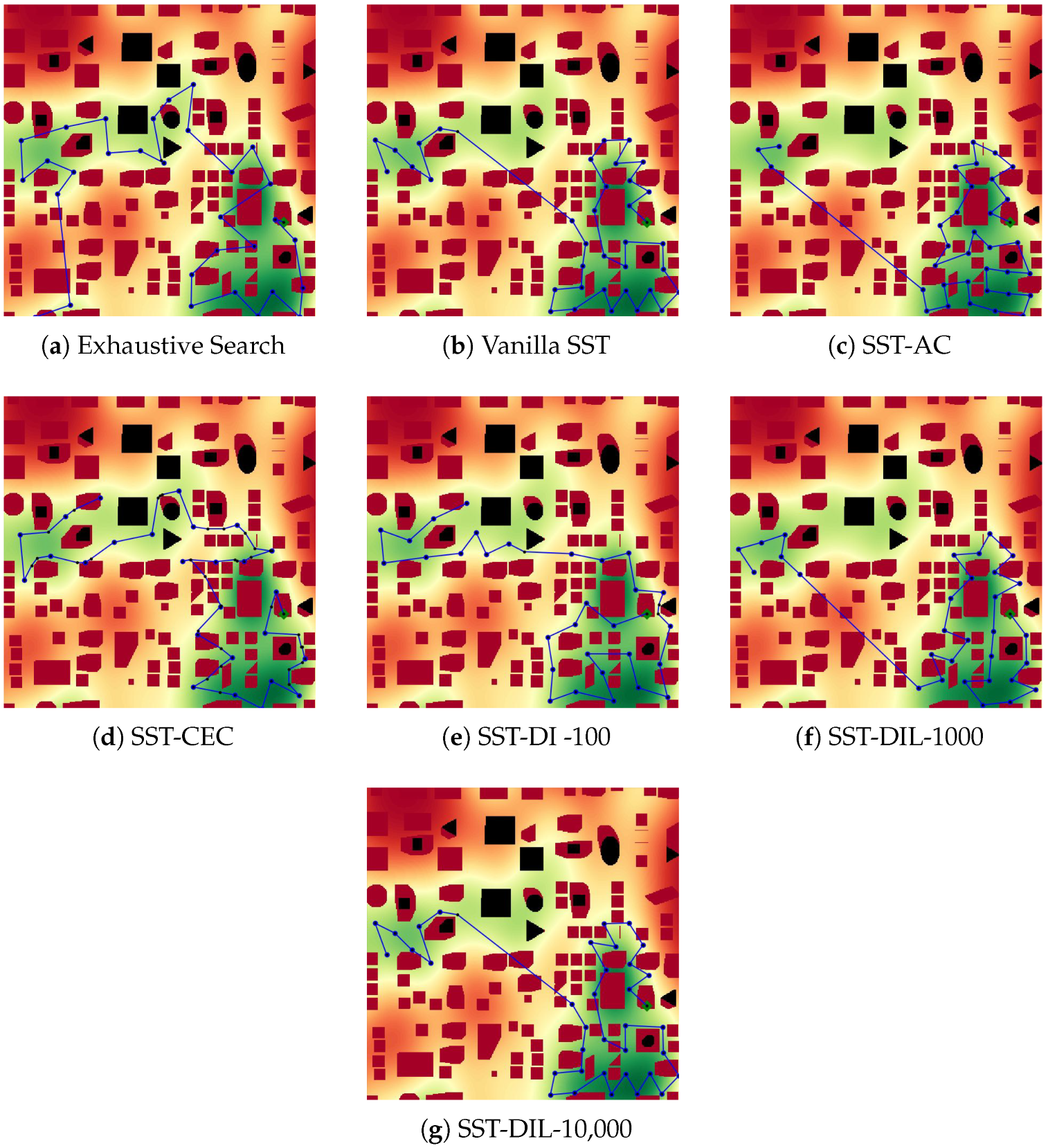
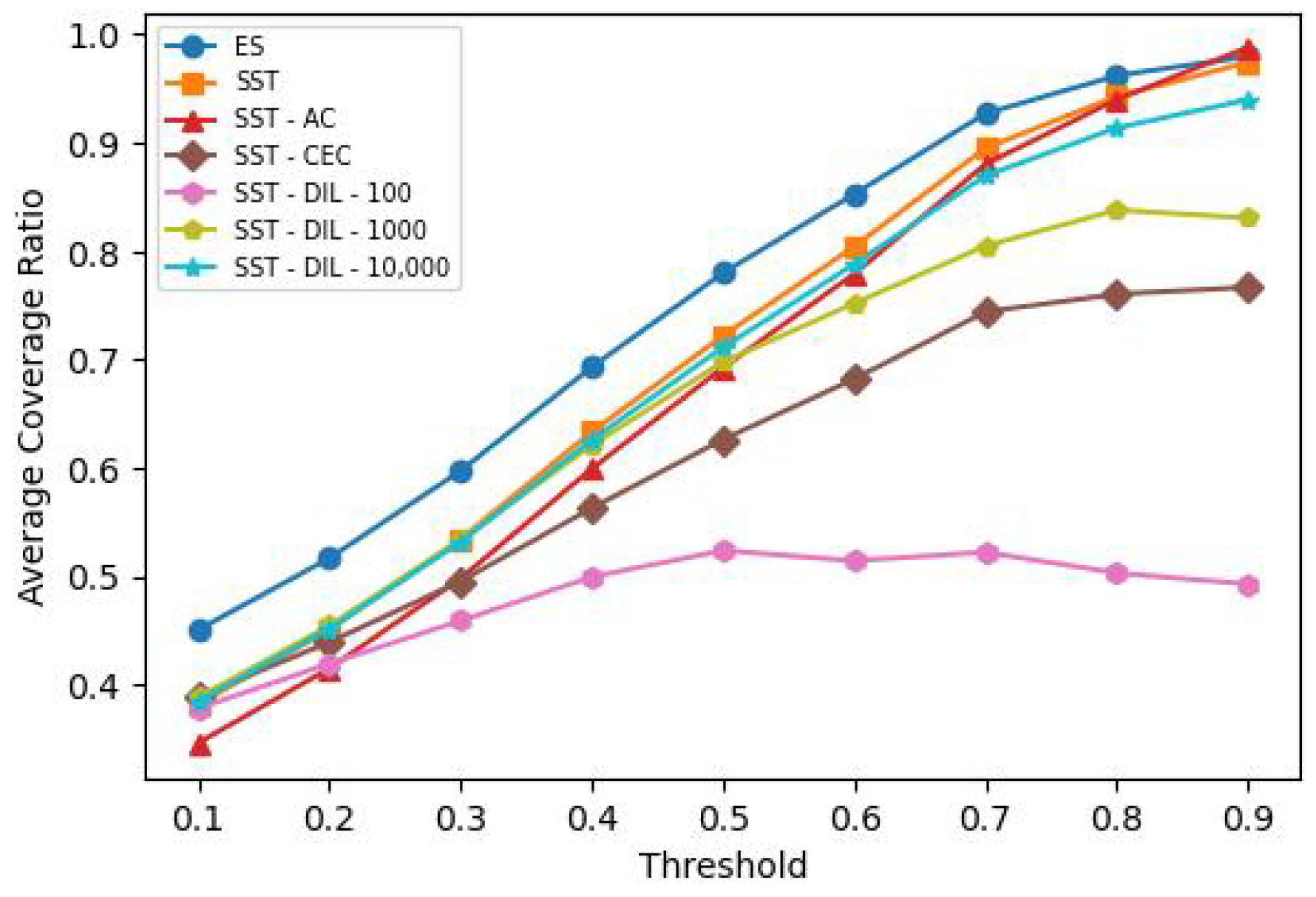
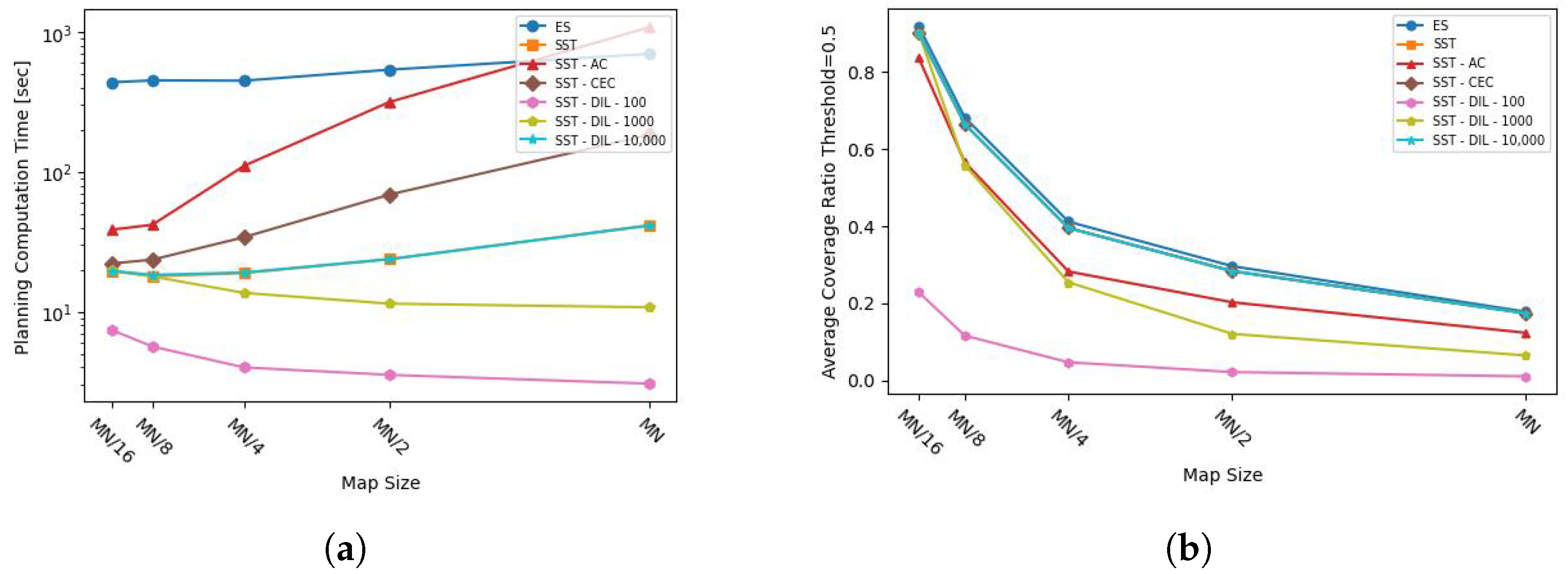
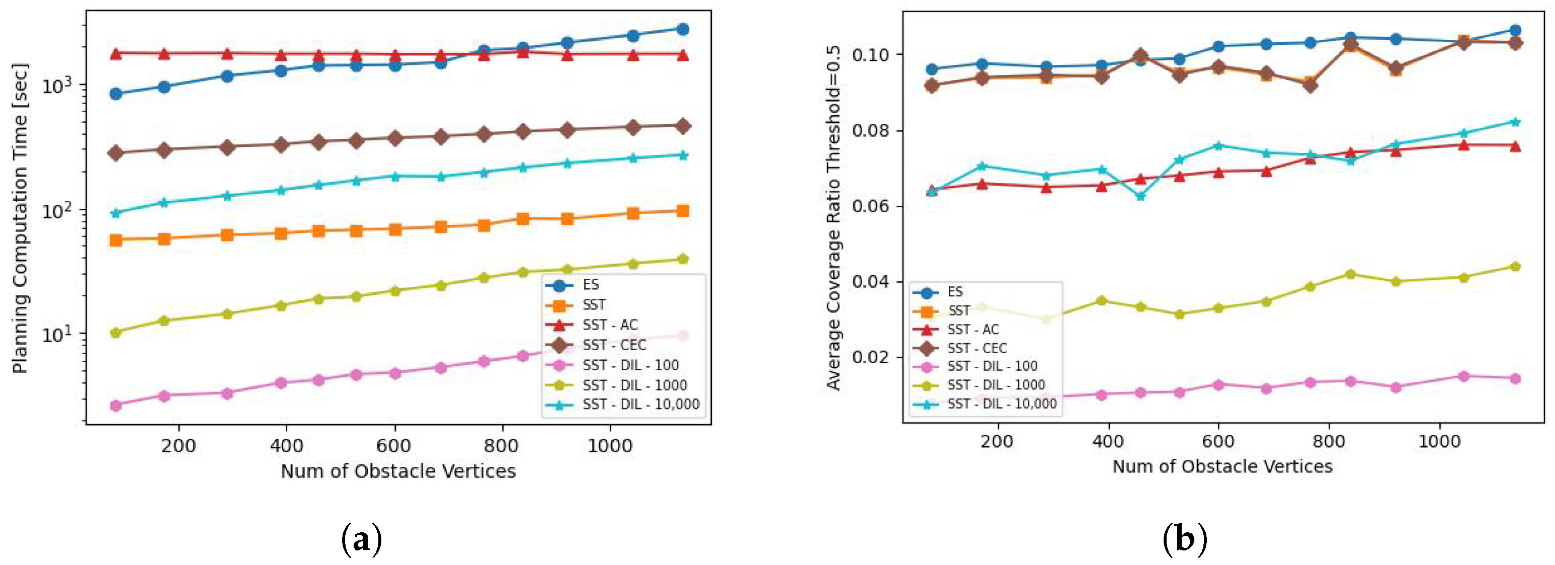
The performance of the algorithms was compared using a simulation study. Not surprisingly, our experiments showed that some variations of the SST algorithm can significantly outperform the baseline heuristic in terms of computational times. Although being best in terms of coverage, ES and SST-AC were seen to be computationally expensive, making them unsuitable for almost real-time performance. On the other hand, the coverage performance of the vanilla SST algorithm was sufficiently close to that of ES, hence providing a good tradeoff between computation times and coverage.

Further work should probably be directed at deepening the way we dilute the set of candidate waypoints, in particular by considering using previously planned trajectories. To improve the exhaustion of time constraints, a fast-to-compute, tighter upper bound for the trajectory length should be developed. Lastly, since the proposed algorithm contains several parts that can be computed in parallel, the use of a GPU should be considered to reduce computation times in actual implementations.