Connectivity Preservation and Obstacle Avoidance Control for Multiple Quadrotor UAVs with Limited Communication Distance

Abstract

This paper studies the distributed formation control problem for multiple unmanned aerial vehicles (UAVs), focusing on preserving connectivity and avoiding obstacles within the constraints of a limited communication distance and in the presence of multiple dynamic obstacles. The UAV network is modeled as a proximity graph, where the edges are defined by the distances between the UAVs. A hierarchical control strategy is employed to manage the position and attitude subsystems independently. A distributed position formation controller is developed for the position subsystems, utilizing bounded artificial potential functions to preserve the network connectivity and avoid collisions between UAVs while achieving the desired formation. The position controller also integrates a time-varying sliding manifold and obstacle avoidance potential functions to prevent collisions with dynamic obstacles. Additionally, an attitude controller is designed for the attitude subsystem to track the desired attitude angles generated by the positioning subsystem. Numerical simulations validate that the proposed controllers effectively preserve the communication network’s connectivity, avoid collisions between the UAVs and dynamic obstacles, and achieve the desired formation simultaneously.

1. Introduction

In recent years, academic interest in multiple unmanned aerial vehicles (UAVs) has surged, driven by their potential applications in areas such as remote sensing, search and rescue, traffic monitoring, multi-lifting, and video surveillance [1,2,3,4,5,6,7]. Unlike a single UAV, multiple UAVs can operate in parallel, making them more efficient in tasks like large-area surveillance or search and rescue in a collapsed building [8,9,10,11,12]. Research on the formation control of multiple UAVs has intensified, with a significant shift from centralized to distributed control approaches [13,14]. However, developing distributed formation controllers remains a challenge, as each UAV has access only to local information.

The connectivity of the communication network is crucial in designing a distributed controller for multiple quadrotor UAVs. Many of the existing studies have traditionally presupposed the connectivity of the communication graph, whether directed or undirected, throughout the formation control processes of UAV clusters [15,16]. For instance, ref. [16] presented a robust distributed formation control method for quadrotor teams, addressing communication delays, nonlinear dynamics, and external disturbances and achieving finite-time convergence of the tracking errors, with experimental validation. Similarly, the work in [17] outlines a hierarchical distributed formation tracking control algorithm for leader-following quadrotors, ensuring asymptotic stability, and demonstrates its effectiveness through simulations and experiments. Event-triggered time-varying or time-invariant formation controllers were also developed for multiple UAVs in [18,19]. Additionally, ref. [20] proposed a collision-resilient control scheme for quadrotors which incorporated a nonlinear disturbance observer and a tilt–torsion decomposition-based attitude controller and was validated through simulations and flight tests. Fault detection and fault-tolerant cooperative control strategies were proposed in [21] for multiple UAVs under actuator faults, sensor faults, and wind disturbances. The distributed formation control design problem for multiple UAVs with a switching interaction topology was studied further in [22,23,24], where the graph was jointly connected. However, the implementation of connectivity in distributed formation control has often been overlooked, with many studies assuming continuous [25,26] or intermittent [27,28] network connectivity.

Due to the limited communication range and mobility of UAVs, disruptions in the communication network can occur, hindering formation control of UAVs. Therefore, ensuring network connectivity is essential when designing distributed formation controllers for multiple UAVs. Connectivity preservation control refers to the process of ensuring that the communication network among multiple agents remains intact and functional by preserving appropriate relative distances and avoiding obstacles, even in dynamic environments. Preserving the connectivity assumptions is challenging in the presence of a limited communication range.Over the past decade, extensive research has been conducted on connectivity preservation in multi-agent systems [29,30]. Nevertheless, most of the existing results have focused on first-order [31] and second-order models [32,33,34,35] without addressing the connectivity preservation problems in nonlinear dynamic systems, such as those in UAV applications. The issue of connectivity preservation for multiple UAVs presents distinct challenges compared to multi-agent systems in two primary ways [36]. While most studies on multi-agent systems have focused on achieving a consensus, connectivity preservation in UAV formation control must account for the complexities of the formation-specific objectives. Unlike the predominantly linear modeling of multi-agent systems, UAV formation control deals with nonlinear dynamics, adding further complexity to connectivity maintenance. Recently, a local connectivity preservation controller for multi-quadrotor aircraft was studied. Recent efforts have introduced local connectivity preservation controllers for multi-quadrotor UAVs [37], as well as a novel approach to maintaining connectivity in UAV systems with bounded actuation and a limited communication range [36]. Recently, advanced decision-making models for connected autonomous vehicles (CAVs) focusing on human-like driving behaviors, game-theoretic frameworks, and risk assessments to enhance lane change decisions, coordination at unsignalized intersections, and interactions with human-driven vehicles in mixed traffic environments were proposed in [38,39,40]. However, the above literature did not consider the effect of obstacles.

Obstacle avoidance is another problem to address when controlling multiple UAVs. Designing distributed controllers that account for obstacles adds complexity, but recent studies have made progress in achieving the desired UAV formations despite these difficulties [41,42,43]. Moreover, when UAVs perform obstacle avoidance tasks, the communication network’s connectivity may be compromised. Therefore, it is crucial to simultaneously address connectivity preservation and obstacle avoidance in the design of distributed controllers for multiple UAVs. Some research has approached this issue. For example, a bounded controller for a multi-robot system was developed to preserve the network connectivity in the presence of obstacles [44]. Similarly, an adaptive tracking control scheme for spacecraft formation flying integrated inter-collision avoidance, obstacle dodging, and connectivity preservation [45]. Other studies have investigated time-varying output formation tracking problems with collision avoidance, obstacle dodging, and connectivity preservation in high-order multi-agent systems [46]. However, these works have been limited by their focus on static obstacles. The central challenge of this work is to develop a distributed connectivity preservation and obstacle avoidance controller for multiple UAVs, specifically in the context of dynamic obstacles.

Motivated by the practical challenges of preserving connectivity and avoiding dynamic obstacles in UAV formations, this paper presents a distributed controller for multiple quadrotor UAVs with communication distance limitations and multiple dynamic obstacles. The approach involves developing a novel formation potential function and an obstacle avoidance potential function, which, combined with a sliding mode control method, enable the design of a distributed position controller. This controller ensures network connectivity, prevents collisions between the UAVs and obstacles, and achieves the desired formation. Additionally, an attitude tracking controller is designed to generate the required control forces, ensuring accurate attitude tracking. Together, these elements address the core challenges of connectivity preservation, obstacle avoidance, and formation control in dynamic environments.

This paper offers three key contributions:

(1)

Unlike traditional distributed cooperative controllers [47,48,49] that assume a continuously connected network, the proposed connectivity preservation method only requires an initially connected network, even with communication distance limitations.

(2)

While previous studies like [37] have focused solely on collision avoidance and connectivity preservation among UAVs, this controller also tackles obstacle avoidance between UAVs and external obstacles.

(3)

In contrast to the existing static obstacle avoidance schemes reviewed in [44,45,46], the proposed control law addresses dynamic obstacle avoidance by utilizing dynamic surface control and a repulsive potential function. This work represents one of the first approaches to simultaneously handling the distributed control of quadrotor UAVs, connectivity preservation, and dynamic obstacle avoidance.

This paper is organized as follows: Section 2 outlines the position and attitude dynamics of quadrotor UAVs and proposes a dynamic communication network model. In Section 3, the potential functions and the distributed position controller are developed, followed by the attitude tracking controller in Section 3.3. Section 4 presents numerical simulations to validate the efficacy of the controllers. Finally, this paper concludes with a summary in Section 5.

2. Preliminaries and the Problem Statement

This section introduces the dynamics of quadrotor UAVs and presents key concepts from algebraic graph theory. In addition, a dynamic graph model of the UAVs’ communication network is developed.

2.1. The Dynamics of Quadrotor UAVs

Consider two reference frames: (1) an inertial frame ${\mathcal{F}}_I=\left\{O_I{x}_I{y}_I{z}_I\right\}$, whose origin $O_I$ is fixed at a specific point on Earth, and (2) a body frame ${\mathcal{F}}_{B_i}=\left\{O_{B_i}{x}_{B_i}{y}_{B_i}{z}_{B_i}\right\}$, whose origin $O_{B_i}$ coincides with the fuselage center of gravity of the ith UAV. The relations between these two frames are shown in Figure 1. The position dynamics of the ith UAV in the inertial frame ${\mathcal{F}}_I$ can be modeled as [37,50]

$$\begin{array}{cc}\hfill m_i{\ddot{\mathit{p}}}_i& =-{\mathit{D}}_i{\dot{\mathit{p}}}_i-m_{i}g{\mathit{e}}_3+T_i{\mathit{R}}_i{\mathit{e}}_3,i=1,\dots ,N\hfill \end{array}$$

(1)

where $m_i$ denotes the total mass of the ith UAV; ${\mathit{p}}_i={[p_{i,x},p_{i,y},p_{i,z}]}^{\top }$ represents its position; ${\dot{\mathit{p}}}_i={[{\dot{\mathit{p}}}_{i,x},{\dot{\mathit{p}}}_{i,y},{\dot{\mathit{p}}}_{i,z}]}^{\top }$ is the velocity; ${\ddot{\mathit{p}}}_i={[{\dot{\mathit{p}}}_{i,x},{\dot{\mathit{p}}}_{i,y},{\dot{\mathit{p}}}_{i,z}]}^{\top }$ is the acceleration in the inertial frame ${\mathcal{F}}_I$; ${\mathit{D}}_i=\mathrm{Diag}(D_{i,x},D_{i,y},D_{i,z})$ represents the aerodynamic damping coefficients; g = 9.81 m/s² is referred to as the acceleration of gravity; and ${\mathit{e}}_3={[0,0,1]}^{\top }\in {\mathbb{R}}^3$. N denotes the number of UAVs. The term $T_i$ is the total lift generated by the four propellers, and ${\mathit{R}}_i$ is the rotation matrix that transforms the vectors from the body ${\mathcal{F}}_{B_i}$ into the inertial frame ${\mathcal{F}}_I$, expressed as

$$\begin{array}{c}\hfill {\mathit{R}}_i=\left[\begin{array}{ccc}cos{\theta }_{i}cos{\psi }_i& sin{\varphi }_{i}sin{\theta }_{i}cos{\psi }_i-cos{\varphi }_{i}sin{\psi }_i& cos{\varphi }_{i}sin{\theta }_{i}cos{\psi }_i+sin{\varphi }_{i}sin{\psi }_i\\ cos{\theta }_{i}sin{\psi }_i& sin{\varphi }_{i}sin{\theta }_{i}sin{\psi }_i+cos{\varphi }_{i}cos{\psi }_i& cos{\varphi }_{i}sin{\theta }_{i}sin{\psi }_i-sin{\varphi }_{i}cos{\psi }_i\\ -sin{\theta }_i& sin{\varphi }_{i}cos{\theta }_i& cos{\varphi }_{i}cos{\theta }_i\end{array}\right]\end{array},$$

where ${\theta }_i,{\varphi }_i$, and ${\psi }_i$ denote the roll, pitch, and yaw angles, respectively.

Given that the position dynamics are influenced by the attitude, the attitude can be treated as a virtual control for the system. To simplify the design of the position controller, we define a virtual input ${\mathit{u}}_i$ as follows [51,52]:

$${\mathit{u}}_i:=T_i{\mathit{R}}_i{\mathit{e}}_3-m_{i}g{\mathit{e}}_3.$$

(2)

Substituting Equation (2) into the original position dynamics Equation (1), the position dynamics can be rewritten as

$$\begin{array}{cc}\hfill m_i{\ddot{\mathit{p}}}_i& =-{\mathit{D}}_i{\dot{\mathit{p}}}_i+{\mathit{u}}_i.\hfill \end{array}$$

(3)

This reformulated equation simplifies the design of the position control law by isolating ${\mathit{u}}_i$ as the key control variable.

For the attitude dynamics, the Euler angles of the ith UAV are denoted by ${\mathit{\eta }}_i=({\varphi }_i,{\theta }_i,{\psi }_i)$, where ${\varphi }_i$, ${\theta }_i$, and ${\psi }_i$ represent the roll, pitch, and yaw, respectively. The angular velocity ${\omega }_i={[{\omega }_{i,x},{\omega }_{i,y},{\omega }_{i,z}]}^{\top }$ is expressed in the body frame ${\mathcal{F}}_{B_i}$. The attitude dynamics can be described as follows [51]:

$$\begin{array}{cc}\hfill & {\dot{\mathit{\eta }}}_i={\mathbf{\Phi }}_i\left({\mathit{\eta }}_i\right){\omega }_i,\hfill \\ \hfill & {\mathit{M}}_i\left({\mathit{\eta }}_i\right)\ddot{{\mathit{\eta }}_i}+{\mathit{C}}_i({\mathit{\eta }}_i,\dot{{\mathit{\eta }}_i})\dot{{\mathit{\eta }}_i}=\mathbf{\Psi }{\left({\mathit{\eta }}_i\right)}^{\top }{\mathit{\tau }}_i,\hfill \end{array}$$

(4)

where ${\mathit{M}}_i\left({\mathit{\eta }}_i\right)={\mathbf{\Psi }}_i{\left({\mathit{\eta }}_i\right)}^{\top }{\mathit{J}}_i{\mathbf{\Psi }}_i\left({\mathit{\eta }}_i\right)$; ${\mathit{J}}_i$ is the inertial matrix of the UAV described in the body frame ${\mathcal{F}}_{B_i}$; ${\mathbf{\Psi }}_i\left({\mathit{\eta }}_i\right)={\mathbf{\Phi }}_i^{-1}\left({\mathit{\eta }}_i\right)$ where ${\mathbf{\Phi }}_i\left({\mathit{\eta }}_i\right)$ is a transformation matrix related to the Euler angles; ${\mathit{\tau }}_i$ represents the torque produced by the four rotors in the body frame ${\mathcal{F}}_{B_i}$; and the Euler matrix ${\Phi }_i\left({\mathit{\eta }}_i\right)$ is given by

$${\mathbf{\Phi }}_i\left({\mathit{\eta }}_i\right)=\left[\begin{array}{ccc}1& sin{\varphi }_{i}sin{\theta }_i/cos{\theta }_i& cos{\varphi }_{i}sin{\theta }_i/cos{\theta }_i\\ 0& cos{\varphi }_i& -sin{\varphi }_i\\ 0& sin{\varphi }_i/cos{\theta }_i& cos{\varphi }_i/cos{\theta }_i\end{array}\right].$$

The Coriolis and centrifugal matrix ${\mathit{C}}_i({\mathit{\eta }}_i,\dot{{\eta }_i})$ for the ith UAV is given by

$${\mathit{C}}_i({\mathit{\eta }}_i,\dot{{\mathit{\eta }}_i})=-\mathbf{\Psi }{\left({\mathit{\eta }}_i\right)}^{\top }{\mathit{J}}_i\dot{\mathbf{\Psi }}\left({\mathit{\eta }}_i\right)+\mathbf{\Psi }{\left({\mathit{\eta }}_i\right)}^{\top }{[\mathbf{\Psi }\left({\mathit{\eta }}_i\right)\dot{{\mathit{\eta }}_i}]}^{\times }{\mathit{J}}_i\mathbf{\Psi }\left({\mathit{\eta }}_i\right),$$

(5)

where ${\mathit{x}}^{\times }$ is a skew symmetric matrix and is defined as follows:

$${\mathit{x}}^{\times }=\left[\begin{array}{ccc}0& -x_3& x_2\\ x_3& 0& -x_1\\ -x_2& x_1& 0\end{array}\right].$$

This matrix accounts for the Coriolis and centrifugal forces acting on the UAV, considering its angular velocity ${\dot{\mathit{\eta }}}_i$ and the inertia matrix ${\mathit{J}}_i$.

Remark 1. 

As shown in (3), the real-time distances between the UAVs determine the elements of the adjacency matrix in (6). The key challenge in designing a distributed controller is how to preserve the connectivity of this dynamic graph throughout operation, ensuring that the communication network remains functional despite changes in the UAVs’ positions.

2.2. Dynamic Communication Network Modeling

The dynamic communication network plays a crucial rule in the distributed formation control of multiple UAVs. The network of all UAVs can be modeled using a distance-induced proximity graph. This proximity graph is represented as $\mathcal{G}(\mathcal{V},\mathcal{E})$, where $\mathcal{V}=\{1,2,\dots ,N\}$ denotes the vertex set, corresponding to the UAVs, and $\mathcal{E}\subset \mathcal{V}\times \mathcal{V}$ denotes the edge set, representing the communication links between the UAVs. In a graph, a path is characterized by a sequence of connected edges, such as $(i_1,i_2),(i_2,i_3),\dots$, where each edge $(i_k,i_{k+1})$ belongs to the set $\mathcal{E}$ with $k=1,2,\cdots$. The graph $\mathcal{G}$ is referred to as connected when there is at least one path linking any two vertices in $\mathcal{V}$. The communication between the UAVs and the detection between UAVs and obstacles are shown in Figure 2. UAVs within the communication range can communicate with each other, and when an obstacle enters the detection range of the UAV, the UAV can obtain information about the obstacle.

Suppose that all UAVs share the same communication distance $\Delta$, and the minimum allowable distance between UAV i and j is denoted by ${\delta }_{ij}$. When the distance between UAVs i and j falls below $\Delta$ but exceeds ${\delta }_{ij}$, then the edge $(i,j)$ is included in the edge set $\mathcal{E}$. If not, the edge $(i,j)$ is excluded from $\mathcal{E}$. Using the definition of the edge, the corresponding adjacency matrix $\mathit{A}\left(\mathcal{G}\right)=\left[a_{ij}\right]\in {\mathbb{R}}^{N\times N}$ for the graph $\mathcal{G}$ is defined as

$$a_{ij}\left(t\right)=\left\{\begin{array}{cc}1,\hfill & \mathrm{if}\left|\right|{\mathit{p}}_{ij}\left(t\right)\left|\right|\in ({\delta }_{ij}+ϵ,\Delta -ϵ),i,j\in \mathcal{V}\},\hfill \\ 0,\hfill & \mathrm{otherwise},\hfill \end{array}\right.$$

(6)

where ${\mathit{p}}_{ij}\left(t\right)={\mathit{p}}_i\left(t\right)-{\mathit{p}}_j\left(t\right)$ denotes the relative displacement of UAVs i and j, and $ϵ>0$ is a small constant. The Laplacian matrix $\mathit{L}\left(\mathcal{G}\right)=\left[l_{ij}\right]\in {\mathbb{R}}^{N\times N}$ is defined using the adjacency matrix $\mathit{A}\left(\mathcal{G}\right)$ as follows:

$$l_{ij}=\left\{\begin{array}{cc}{\sum }_{j=1}^N{a}_{ij},\hfill & \mathrm{if}i=j,\hfill \\ -a_{ij},\hfill & \mathrm{otherwise}.\hfill \end{array}\right.$$

Suppose the minimum allowable distance between UAV i and obstacle k is ${\delta }_{ik}^o$. When the distance between UAV i and obstacle l falls below $\Delta$ but exceeds ${\delta }_{ik}^o$, then the edge $(i,k)$ is included in the edge set ${\mathcal{E}}^o$. If not, the edge $(i,k)$ is excluded from ${\mathcal{E}}^o$. The adjacency matrix $\mathit{B}=\left[b_{ik}\right]\in {\mathbb{R}}^{N\times M}$ characterizes the interactions between UAV i and obstacle k and is defined as follows:

$$b_{ik}\left(t\right)=\left\{\begin{array}{cc}1,\hfill & \mathrm{if}\left|\right|{\mathit{p}}_{ik}^o\left(t\right)\left|\right|\in ({\delta }_{ik}^o+ϵ,\Delta -ϵ),i\in \mathcal{V},k\in {\mathcal{V}}^o\},\hfill \\ 0,\hfill & \mathrm{otherwise},\hfill \end{array}\right.$$

(7)

where ${\mathit{p}}_{ik}^o\left(t\right)={\mathit{p}}_i\left(t\right)-{\mathit{p}}_k^o\left(t\right)$ denotes the displacement between UAV i and obstacle k, ${\mathcal{V}}^o$ denotes the set of the obstacles, and M denotes the number of obstacles.

Remark 2. 

In this study, we consider the communication distance limitation because it significantly impacts the performance of distributed controllers for multiple UAVs. The communication distance affects the reliability of data transmission, and factors like long distances or bad weather can cause packet loss, delays, or reduced quality. As a result, UAVs typically have a limited reliable communication range. While the focus of this research is on theoretical modeling and control strategies, considering the communication distance is crucial for improving the practical application of the system in dynamic environments. Including these limitations makes the work more relevant to real-world engineering challenges.

2.3. The Control Objective

Our objective in this paper is to engineer a distributed controller that directs the quadrotor UAVs into a desired formation, overcoming limitations such as restricted communication distances and moving obstacles. We establish our controller design based on this crucial lemma and several assumptions:

Lemma 1. 

If the graph $\mathcal{G}$ is connected, then its Laplacian matrix $\mathit{L}\left(\mathcal{G}\right)$ is positive semidefinite [53].

Assumption 1. 

As stipulated by (6), the initial graph $\mathcal{G}\left(0\right)$ is inherently a connected graph.

Assumption 2. 

The desired formation ${\mathit{p}}_d$ must adhere to the following criteria:

$$\begin{array}{cc}\hfill d_{ij}<& \Delta ,\forall i\in \{1,\dots ,N\},j\in {\mathcal{N}}_i,\hfill \\ \hfill d_{ij}>& {\delta }_{ij},\forall i,j\in \{1,\dots ,N\},\hfill \end{array}$$

where $d_{ij}=\left|\right|{\mathit{p}}_i^d-{\mathit{p}}_j^d\left|\right|$ denotes the intended distance between UAVs i and j.

Assumption 3. 

Obstacles impact the UAVs temporarily, with their effects limited to a bounded duration, and their velocities remain within a defined range.

Remark 3. 

In the prevailing research on distributed formation control of UAVs, it is commonly accepted that the network remains consistently connected [47,48,49,54,55]. Contrarily, Assumption 1 modifies this to require only initial connectivity rather than continuous connectivity. Assumption 2, also referenced in [44], confirms that the specified formation is achievable. Furthermore, Assumption 3 guarantees that obstacles do not prevent UAVs from attaining the desired formation, substantiating the validity of these assumptions.

3. Distributed Controller Design

The control system for the quadrotor UAVs is segregated into position and attitude subsystems, acknowledging the cascading characteristics of these vehicles. The distributed formation controller for the position subsystem is derived using a series of novel artificial potential functions and the dynamic surface control technique. Figure 3 shows the working process of the proposed connectivity preservation controllers.

3.1. Artificial Potential Functions

Two artificial potential functions were developed: a formation potential function, $P_{ij}^f$, and an obstacle avoidance potential function, $P_{ik}^o$. The function $P_{ij}^f$ is used to preserve connectivity in the network, the collisions between the UAVs, and the desired formation. The formation potential function $P_{ij}^f$ is defined according to the initial distance between two UAVs.

(1)

If $∥{\mathit{p}}_{ij}\left(0\right)∥\in [{\delta }_{ij},\Delta )$, $P_{ij}^f$ is defined as follows [56,57]:

$$P_{ij}^f\left(∥{\mathit{p}}_{ij}∥\right)=\left\{\begin{array}{cc}{P}^r\left(∥{\mathit{p}}_{ij}∥\right),\hfill & ∥{\mathit{p}}_{ij}\left(t\right)∥\in \left({\delta }_{ij},d_{ij}\right]\hfill \\ P^a\left(∥{\mathit{p}}_{ij}∥\right),\hfill & ∥{\mathit{p}}_{ij}\left(t\right)∥\in \left[d_{ij},\Delta \right)\hfill \end{array}\right.,$$

where $P^r\left(∥{\mathit{p}}_{ij}∥\right)$ denotes the repulsive potential function, and $P^a\left(∥{\mathit{p}}_{ij}∥\right)$ represents the attractive potential function, with both mediating the interactions between UAVs based on their distances. The three potential functions satisfy the following conditions:

(a)

$P_{ij}^f\left(∥{\mathit{p}}_{ij}∥\right)$ is a continuous and differentiable nonnegative function of $\left|\right|{\mathit{p}}_{ij}\left(t\right)\left|\right|$;

(b)

$P_{ij}^f\left(∥{\mathit{p}}_{ij}∥\right)$ is symmetric and achieves its unique minimum while $\left|\right|{\mathit{p}}_{ij}\left(t\right)\left|\right|=d_{ij}$;

(c)

$P^r\left(∥{\mathit{p}}_{ij}∥\right)$ monotonically decreases with respect to $\parallel {\mathit{p}}_{ij}\parallel$, and $P_{ij}^r\to \infty$ as $\left|\right|{\mathit{p}}_{ij}\left(t\right)\left|\right|\to {\delta }_{ij}$;

(d)

$P^a\left(∥{\mathit{p}}_{ij}∥\right)$ monotonically decreases with respect to $∥{\mathit{p}}_{ij}∥$, and $P_{ij}^a\to \infty$ as $\left|\right|{\mathit{p}}_{ij}\left(t\right)\left|\right|\to \Delta$.

(2)

If $∥{\mathit{p}}_{ij}\left(0\right)∥\in (\Delta ,\infty )$, $P_{ij}^f$ is defined as [56,57]

$$P_{ij}^f\left(∥{\mathit{p}}_{ij}∥\right)=\left\{\begin{array}{cc}{P}^r\left(∥{\mathit{p}}_{ij}∥\right),\hfill & ∥{\mathit{p}}_{ij}\left(t\right)∥\in \left({\delta }_{ij},d_{ij}\right]\hfill \\ P^d\left(∥{\mathit{p}}_{ij}∥\right),\hfill & ∥{\mathit{p}}_{ij}\left(t\right)∥\in \left[d_{ij},\Delta \right)\hfill \\ P^d(\Delta ),\hfill & ∥{\mathit{p}}_{ij}\left(t\right)∥\in [\Delta ,\infty )\hfill \end{array}\right.,$$

where $P^d\left(∥{\mathit{p}}_{ij}∥\right)$ is the desired formation potential function. $P_{ij}^f\left(∥{\mathit{p}}_{ij}∥\right)$ and $P^r\left(∥{\mathit{p}}_{ij}∥\right)$ satisfy the above conditions (a)–(c). $P^d\left(∥{\mathit{p}}_{ij}∥\right)$ monotonically increases with respect to $∥{\mathit{p}}_{ij}∥$, and $P_{ij}^d\to S$ as $\left|\right|{\mathit{p}}_{ij}\left(t\right)\left|\right|\to \Delta$, where S is a positive constant.

The obstacle avoidance potential function, $P_{ik}^o$, is specifically designed to prevent collisions between the UAVs and the dynamic obstacles. The function $P_{ik}^o$ is given as follows [57]:

$$P_{ik}^o\left(∥{\mathit{p}}_{ik}^o∥\right)=\left\{\begin{array}{cc}{P}_{ij}^r\left(∥{\mathit{p}}_{ik}^o∥\right),\hfill & ∥{\mathit{p}}_{ik}^o\left(t\right)∥\in \left({\delta }_{ik}^o+ϵ,d_{ik}^o\right]\hfill \\ 0,\hfill & ∥{\mathit{p}}_{ik}^o\left(t\right)∥\in \left[d_{ik}^o,\infty \right)\hfill \end{array}\right.,$$

where the term $d_{ik}^o$ refers to the critical distance that triggers the obstacle avoidance potential function for UAV i and obstacle k. $P_{ij}^r\left(∥{\mathit{p}}_{ik}^o∥\right)$ satisfies

(1)

$P_{ik}^r\left(\right||{\mathit{p}}_{ik}^o\left(t\right)\left|\right|)$ being a continuous and differentiable nonnegative function of $\left|\right|{\mathit{p}}_{ik}^o\left(t\right)\left|\right|$;

(2)

$P_{ik}^r\left(\right||{\mathit{p}}_{ik}^o\left(t\right)\left|\right|)$ monotonically decreasing with respect to $\left|\right|{\mathit{p}}_{ik}^o\left(t\right)\left|\right|$, while $\left|\right|{\mathit{p}}_{ik}^o\left(t\right)\left|\right|\in [{\delta }_{ik}^o,d_{ik}^o]$;

(3)

$P_{ik}^r\left(\right||{\mathit{p}}_{ik}^o\left(t\right)\left|\right|)\to \infty$ as $\left|\right|{\mathit{p}}_{ik}^o\left(t\right)\left|\right|\to {\delta }_{ik}^o$, and $P_{ik}^r\to 0$ as $\left|\right|{\mathit{p}}_{ik}^o\left(t\right)\left|\right|\to d_{ik}^o$.

3.2. Position Controller Design and Analysis

We define the following coordinate transformation for each UAV:

$${\mathit{s}}_i={\dot{\mathit{p}}}_i-{\widehat{\mathit{v}}}_i(i=1,\dots ,N)$$

(8)

where the engineered virtual velocity item ${\widehat{\mathit{v}}}_i$ is developed to help avoid potential collisions with obstacles as follows:

$${\widehat{\mathit{v}}}_i=-{\nabla }_{{\mathit{p}}_i}P+{\alpha }_2\sum _{k=1}^M{b}_{ik}{\mathit{w}}_{ik},$$

(9)

where the artificial potential function P is defined as follows [57]:

$$\begin{array}{c}\hfill P={\alpha }_1\sum _{i=1}^N\sum _{j=1}^N{a}_{ij}{P}_{ij}^f\left(\right||{\mathit{p}}_{ij}\left(t\right)\left|\right|)+{\alpha }_2\sum _{i=1}^N\sum _{k=1}^M{b}_{ik}{P}_{ik}^o\left(\right||{\mathit{p}}_{ik}^o\left(t\right)\left|\right|),\end{array}$$

(10)

where ${\alpha }_1$ and ${\alpha }_2$ are positive constants, and

$${\mathit{w}}_{ik,q}=\left\{\begin{array}{cc}{\displaystyle \frac{{\left({\nabla }_{{\mathit{p}}_i}{P}_{ik}^o\right)}_q{\dot{\mathit{p}}}_{k,q}^o}{{\left({\nabla }_{{\mathit{p}}_i}P\right)}_q}},\hfill & \mathrm{if}{\left({\nabla }_{{\mathit{p}}_i}{P}_{ik}^o\right)}_q\ne 0,\hfill \\ 0,\hfill & \mathrm{otherwise},\hfill \end{array}\right.q=x,y,z,$$

(11)

where ${\left({\nabla }_{{\mathit{p}}_i}{P}_{ik}^o\right)}_q$ and ${\dot{\mathit{p}}}_{kq}^o$ are the components of ${\nabla }_{{\mathit{p}}_i}{P}_{ik}^o$ and ${\dot{\mathit{p}}}_k^o$ in direction q, respectively.

Remark 4. 

Consider a scenario where $\left({\nabla }_{{\mathit{p}}_i}P\right)q$ is zero, rendering the expression for ${\mathit{w}}_{ik,q}$ undefined due to its reliance on a non-zero denominator. To address this, one can modify the denominator to include a small positive constant ν when zero is encountered. This adjustment is seldom required, however, as the presence of ${\nabla }_{{\mathit{p}}_i}{P}^o$ within ${\nabla }_{{\mathit{p}}_i}P$ usually ensures non-zero values.

Following the introduction of the potential functions, the distributed position controller is constructed as detailed below. This design integrates the essential components of the potential functions to manage the UAVs’ spatial dynamics effectively, focusing on achieving the desired formations while avoiding obstacles and preserving connectivity.

$${\mathit{u}}_i=-{\alpha }_3\sum _{j=1}^N{a}_{ij}({\mathit{s}}_i-{\mathit{s}}_j)-{\alpha }_4{\mathit{s}}_i-{\beta }_i\mathrm{sgn}\left({\mathit{s}}_i\right)-{\nabla }_{{\mathit{p}}_i}P+{\mathit{D}}_i{\dot{\mathit{p}}}_i,$$

(12)

where ${\alpha }_3$, ${\alpha }_4$, and ${\beta }_i$ are positive constants.

We define a low-pass filter in the context of UAV control systems as illustrated in the following equation [58,59]:

$$\lambda {\dot{\mathit{h}}}_i=-{\mathit{h}}_i+{\widehat{\mathit{v}}}_i,$$

(13)

where $\lambda$ is a small constant. This setup allows for a dynamic response where the filter’s output, ${\mathit{h}}_i$, approximates the behavior of the input ${\widehat{\mathit{v}}}_i$ over time.

Selecting an appropriate value for $\lambda$, similar to the methodology in [60], leads to the approximation

$${\mathit{h}}_i\approx {\left[{\widehat{\mathit{v}}}_i\right]}_{eq},$$

(14)

where the subscript “eq” denotes the equivalent value of ${\widehat{\mathit{v}}}_i$. This indicates that ${\mathit{h}}_i$ converges to a value close to the desired velocity input ${\widehat{\mathit{v}}}_i$. Then, we have the following inequality [58]:

$$m_i∥{\displaystyle \frac{\mathrm{d}}{\mathrm{d}t}}{\widehat{\mathit{v}}}_i∥=m_i\left|\right|{\dot{\mathit{h}}}_i\left|\right|\le {\gamma }_i,$$

(15)

where $m_i$ represents the mass of the UAV, and ${\gamma }_i$ is a predefined positive constant that limits the maximum allowable change in velocity, ensuring that the system’s response remains within safe operational limits. According to the decomposition principle of E.S. Pyatnitsky, Equation (15) guarantees the controllability of the Lagrangian dynamical system. This setup effectively filters out high-frequency components from the velocity signals, thus smoothing the UAV’s motion and improving its stability and the control accuracy.

Theorem 1. 

Consider a system defined by (3) involving N UAVs and M dynamic obstacles, with the adjacency matrices derived from Equations (6) and (7). Assuming that Assumptions 1–3 are satisfied and choosing ${\beta }_i>{\gamma }_i$, the implementation of the distributed controller (12) guarantees the achievement of the following objectives:

(1) 

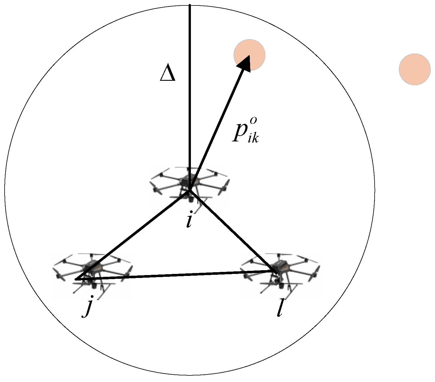
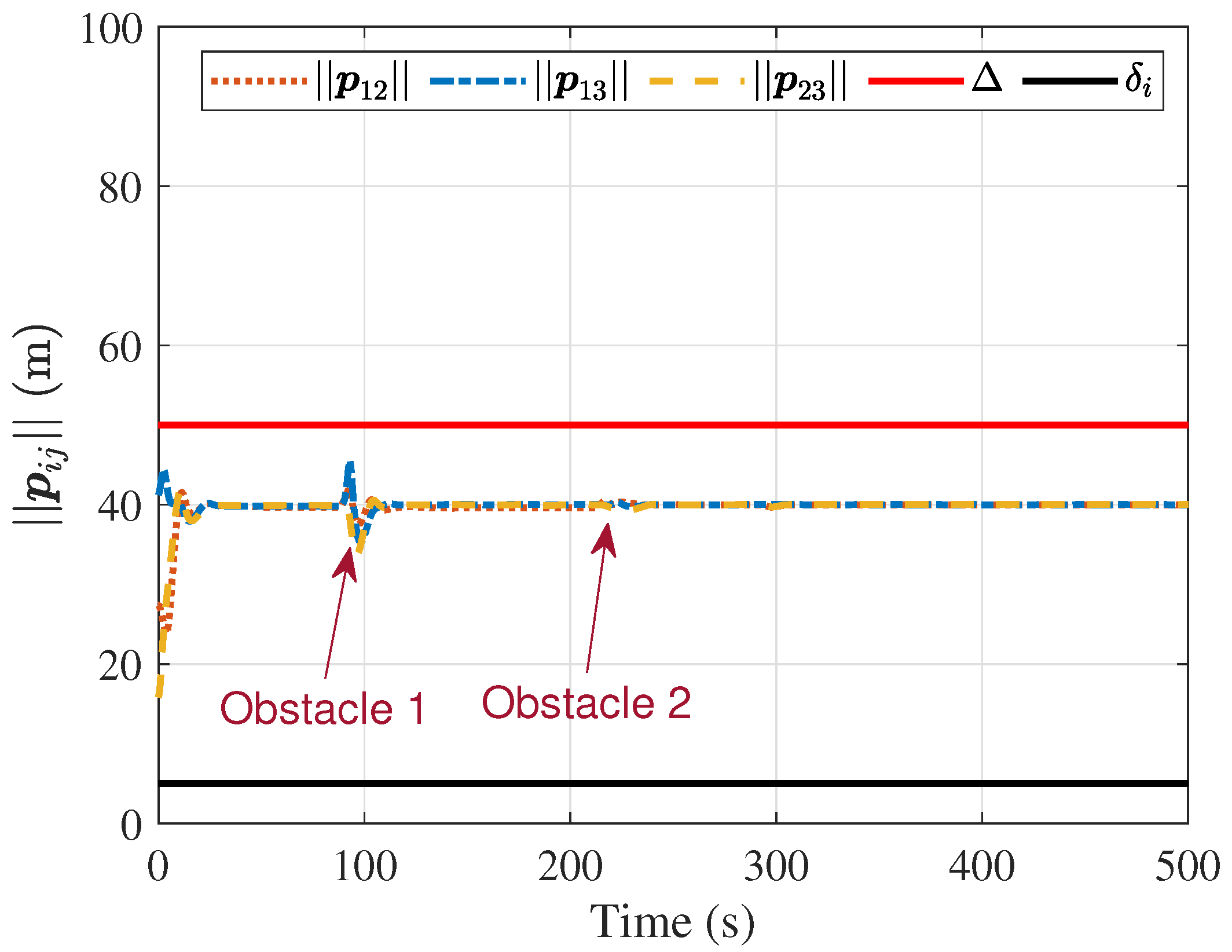
If the initial distance between any two connected UAVs $(i,j)\in \mathcal{E}$ is less than Δ, i.e., $\left|{\mathit{p}}_{ij}\left(0\right)\right|<\Delta$, then $\left|{\mathit{p}}_{ij}\left(t\right)\right|<\Delta$ for all $t>0$;

(2) 

The distance between any two UAVs $i,j\in \mathcal{V}$ remains greater than ${\delta }_{ij}$ at all times, i.e., $\left|{\mathit{p}}_{ij}\left(t\right)\right|>{\delta }_{ij}$ for all $t>0$;

(3) 

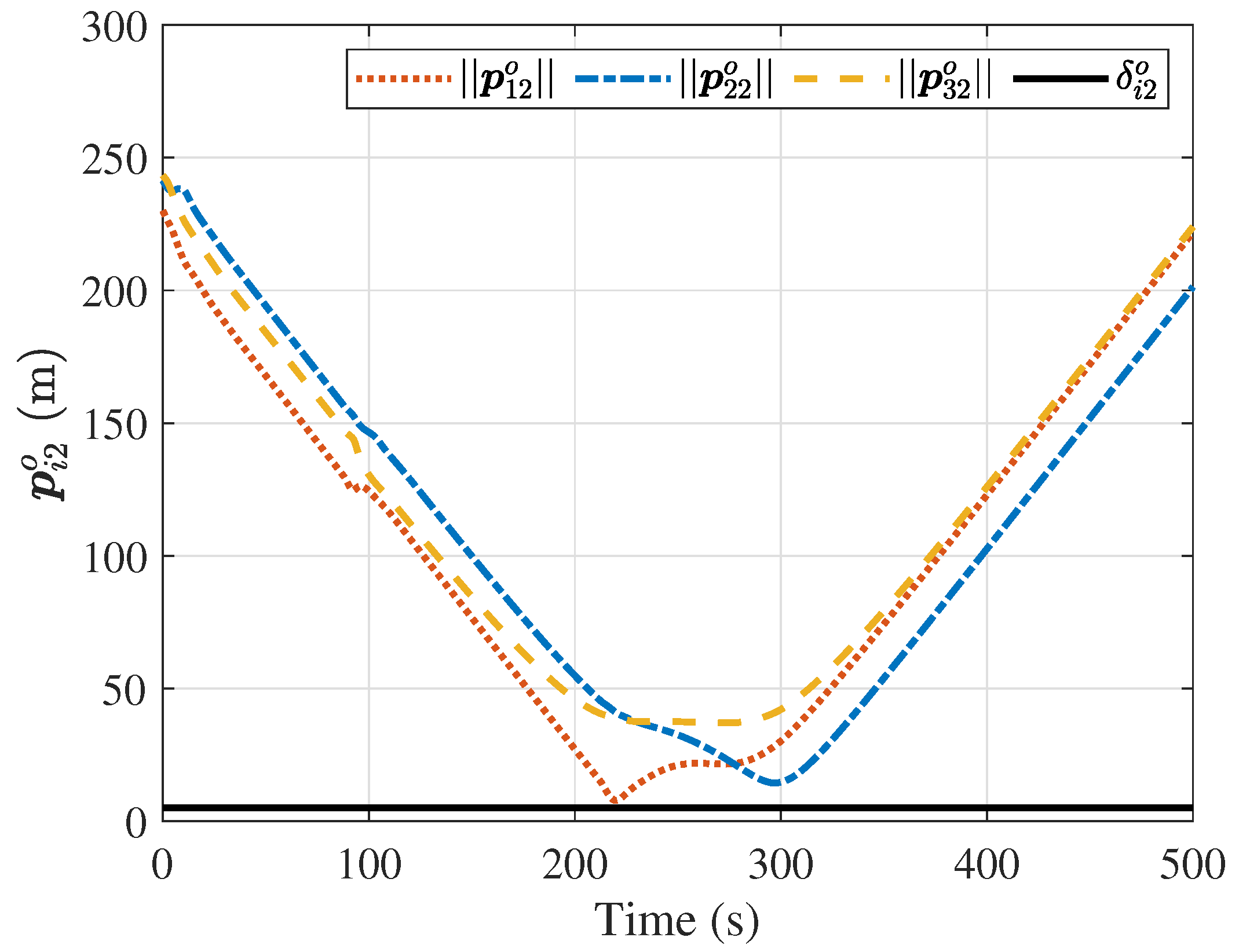
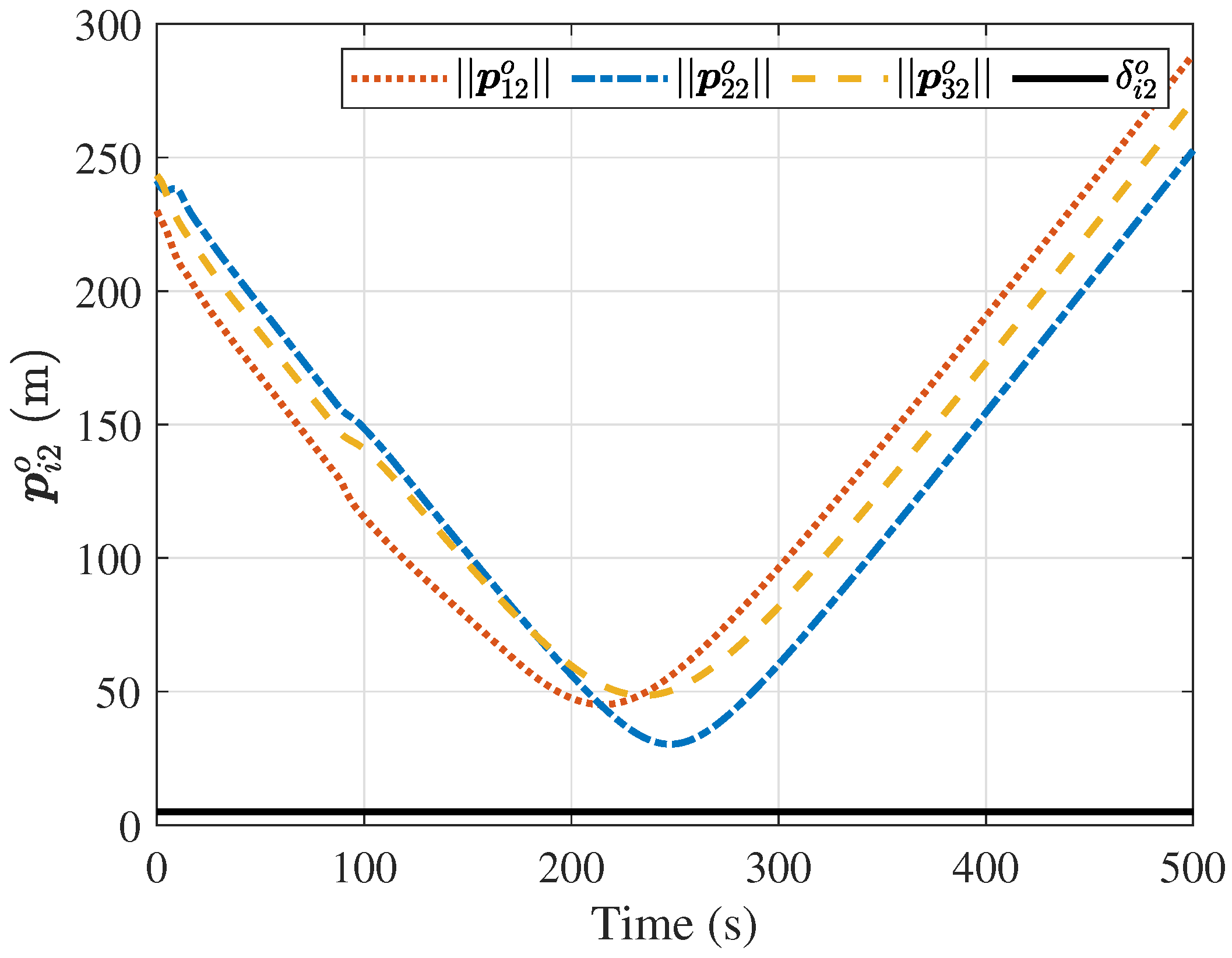
The distance between any UAV $i\in \mathcal{V}$ and any obstacle $k\in {\mathcal{V}}^o$ remains greater than ${\delta }_{ik}^o$ at all times, i.e., $\left|{\mathit{p}}_{ik}^o\left(t\right)\right|>{\delta }_{ik}^o$ for all $t>0$;

(4) 

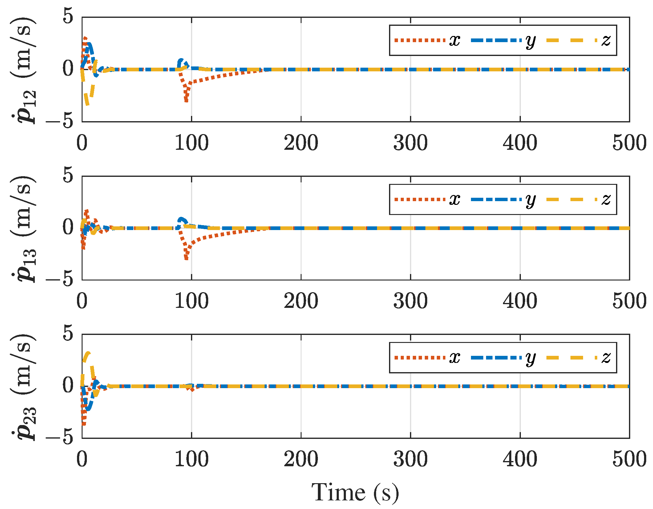
As time progresses towards infinity, the distance between each pair of connected UAVs $(i,j)\in \mathcal{E}$ converges to $d_{ij}$, and the velocity of each UAV $i=1,2,\dots ,N$ approaches zero, i.e., $\left|{\mathit{p}}_{ij}\left(t\right)\right|\to d_{ij}$ and ${\dot{\mathit{p}}}_i\left(t\right)\to 0$ as $t\to \infty$.

Proof. 

Taking the derivative of (8) and scaling both sides by $m_i$,

$$m_i{\dot{\mathit{s}}}_i=m_i{\ddot{\mathit{p}}}_i-m_i{\dot{\widehat{\mathit{v}}}}_i$$

(16)

Next, we integrate the control laws defined in (3) and (12) into the derived equation, resulting in the following comprehensive dynamic model:

$$\begin{array}{cc}\hfill m_i{\dot{\mathit{s}}}_i=& -{\mathit{D}}_i{\dot{\mathit{p}}}_i-{\alpha }_3\sum _{j=1}^N{a}_{ij}({\mathit{s}}_i-{\mathit{s}}_j)-{\alpha }_4{\mathit{s}}_i-{\beta }_i\mathrm{sgn}\left({\mathit{s}}_i\right)-{\nabla }_{{\mathit{p}}_i}P+{\mathit{D}}_i{\dot{\mathit{p}}}_i-m_i{\dot{\widehat{\mathit{v}}}}_i\hfill \\ \hfill =& -{\alpha }_3\sum _{j=1}^N{a}_{ij}({\mathit{s}}_i-{\mathit{s}}_j)-{\alpha }_4{\mathit{s}}_i-{\beta }_i\mathrm{sgn}\left({\mathit{s}}_i\right)-{\nabla }_{{\mathit{p}}_i}P-m_i{\dot{\widehat{\mathit{v}}}}_i\hfill \end{array}$$

(17)

To assess the stability of this dynamic system, we propose the following Lyapunov function candidate:

$$V_1\left(t\right)={\displaystyle \frac{1}{2}}\sum _{i=1}^N{m}_i{\mathit{s}}_i^{\top }{\mathit{s}}_i.$$

(18)

Taking the derivative of (18) and incorporating the results from (17), we derive the following expression for the time derivative of the Lyapunov function:

$$\begin{array}{cc}\hfill {\dot{V}}_1\left(t\right)=& \sum _{i=1}^N{\mathit{s}}_i^{\top }[-{\alpha }_3\sum _{j=1}^N{a}_{ij}({\mathit{s}}_i-{\mathit{s}}_j)-{\alpha }_4{\mathit{s}}_i\hfill \\ \hfill & -{\beta }_i\mathrm{sgn}\left({\mathit{s}}_i\right)-{\nabla }_{{\mathit{p}}_i}P-m_i{\dot{\widehat{\mathit{v}}}}_i]\hfill \\ \hfill =& -{\alpha }_4\sum _{i=1}^N{\mathit{s}}_i^{\top }{\mathit{s}}_i-{\alpha }_3\sum _{i=1}^N\sum _{j=1}^N{a}_{ij}{\mathit{s}}_i^{\top }({\mathit{s}}_i-{\mathit{s}}_j)\hfill \\ \hfill & -\sum _{i=1}^N{\left({\nabla }_{{\mathit{p}}_i}P\right)}^{\top }{\mathit{s}}_i-\sum _{i=1}^N{\mathit{s}}_i^{\top }[{\beta }_i\mathrm{sgn}\left({\mathit{s}}_i\right)+m_i{\dot{\widehat{\mathit{v}}}}_i]\hfill \end{array}$$

(19)

Now, we propose the following Lyapunov function candidate for the stability analysis:

$$V_2\left(t\right)=V_1\left(t\right)+P.$$

(20)

where P denotes the artificial potential function defined in (10).

Taking note of the definition of P and using (19), the derivative of $V_2\left(t\right)$ is computed as

$$\begin{array}{cc}\hfill {\dot{V}}_2\left(t\right)=& -{\alpha }_4\sum _{i=1}^N{\mathit{s}}_i^{\top }{\mathit{s}}_i-{\alpha }_3\sum _{i=1}^N\sum _{j=1}^N{a}_{ij}{\mathit{s}}_i^{\top }({\mathit{s}}_i-{\mathit{s}}_j)\hfill \\ \hfill & -\sum _{i=1}^N{\left({\nabla }_{{\mathit{p}}_i}P\right)}^{\top }{\mathit{s}}_i-\sum _{i=1}^N{\mathit{s}}_i^{\top }[{\beta }_i\mathrm{sgn}\left({\mathit{s}}_i\right)+m_i{\dot{\widehat{\mathit{v}}}}_i]\hfill \\ \hfill & +\sum _{i=1}^N{\left({\nabla }_{{\mathit{p}}_i}P\right)}^{\top }{\dot{\mathit{p}}}_i+\sum _{i=1}^M{\left({\nabla }_{{\mathit{p}}_k^o}P\right)}^{\top }{\dot{\mathit{p}}}_k^o\hfill \\ \hfill =& -{\alpha }_4\sum _{i=1}^N{\mathit{s}}_i^{\top }{\mathit{s}}_i-{\alpha }_3\sum _{i=1}^N\sum _{j=1}^N{a}_{ij}{\mathit{s}}_i^{\top }({\mathit{s}}_i-{\mathit{s}}_j)\hfill \\ \hfill & -\sum _{i=1}^N{\mathit{s}}_i^{\top }[{\beta }_i\mathrm{sgn}\left({\mathit{s}}_i\right)+m_i{\dot{\widehat{\mathit{v}}}}_i]+\sum _{i=1}^N{\left({\nabla }_{{\mathit{p}}_i}P\right)}^{\top }{\widehat{\mathit{v}}}_i+\sum _{i=1}^M{\left({\nabla }_{{\mathit{p}}_k^o}P\right)}^{\top }{\dot{\mathit{p}}}_k^o.\hfill \end{array}$$

(21)

By using (9), Equation (21) can be rewritten as

$$\begin{array}{cc}\hfill {\dot{V}}_2\left(t\right)=& -{\alpha }_4\sum _{i=1}^N{\mathit{s}}_i^{\top }{\mathit{s}}_i-{\alpha }_3\sum _{i=1}^N\sum _{j=1}^N{a}_{ij}{\mathit{s}}_i^{\top }({\mathit{s}}_i-{\mathit{s}}_j)-\sum _{i=1}^N{\mathit{s}}_i^{\top }[{\beta }_i\mathrm{sgn}\left({\mathit{s}}_i\right)+m_i{\dot{\widehat{\mathit{v}}}}_i]\hfill \\ \hfill & -\sum _{i=1}^N{\left({\nabla }_{{\mathit{p}}_i}P\right)}^{\top }\left({\nabla }_{{\mathit{p}}_i}P\right)+{\alpha }_2\sum _{i=1}^N\sum _{k=1}^M{b}_{ik}{\left({\nabla }_{{\mathit{p}}_i}P\right)}^{\top }{\mathit{w}}_{ik}+\sum _{i=1}^M{\left({\nabla }_{{\mathit{p}}_k^o}P\right)}^{\top }{\dot{\mathit{p}}}_k^o.\hfill \end{array}$$

(22)

Pre-multiplying both sides of (11) by ${\left({\nabla }_{{\mathit{p}}_i}P\right)}^{\top }$ yields

$${\left({\nabla }_{{\mathit{p}}_i}P\right)}^{\top }{\mathit{w}}_{ik}={\left({\nabla }_{{\mathit{p}}_i}{P}_{ik}^o\right)}^{\top }{\dot{\mathit{p}}}_k^o=-{\left({\nabla }_{{\mathit{p}}_k^o}{P}_{ik}^o\right)}^{\top }{\dot{\mathit{p}}}_k^o.$$

(23)

Based on (23) and ${\beta }_i>{\gamma }_i$, (22) can be simplified as

$$\begin{array}{cc}\hfill {\dot{V}}_2\left(t\right)=& -{\alpha }_4\sum _{i=1}^N{\mathit{s}}_i^{\top }{\mathit{s}}_i-{\alpha }_3\sum _{i=1}^N\sum _{j=1}^N{a}_{ij}{\mathit{s}}_i^{\top }({\mathit{s}}_i-{\mathit{s}}_j)-\hfill \\ \hfill & \sum _{i=1}^N{\mathit{s}}_i^{\top }[{\beta }_i\mathrm{sgn}\left({\mathit{s}}_i\right)+m_i{\dot{\widehat{\mathit{v}}}}_i]-\sum _{i=1}^N{\left({\nabla }_{{\mathit{p}}_i}P\right)}^{\top }\left({\nabla }_{{\mathit{p}}_i}P\right)\hfill \\ \hfill & \le -\sum _{i=1}^N\left|\right|{\nabla }_{{\mathit{p}}_i}{P\left)\right||}^2-{\alpha }_3\left|\right|\left[\mathit{L}\left(t\right)\otimes {\mathit{I}}_3\right]\left|\right|·{\left|\right|\mathit{s}\left|\right|}^2-{\alpha }_4{\left|\right|\mathit{s}\left|\right|}^2.\hfill \end{array}$$

(24)

The graph $\mathcal{G}\left(t\right)$ is assumed to change only at discrete times $t_k(k=0,1,\dots ,t_0=0)$ and remains static within each interval $\left[t_{k-1},t_k\right)$. Based on Assumption 1 and Lemma 1, the Laplacian matrix $\mathit{L}\left(t\right)$ remains positive semi-definite during $[t_0,t_1)$. Furthermore, we have ${\dot{V}}_2\left(t\right)\le 0$ and $V_2\left(t\right)\le V_2\left(0\right)$ while $t\in [t_0,t_1)$. At $t=t_1$, up to $N(N-1)$ UAV links and $MN$ UAV–obstacle links enrich the potential function P, resulting in $V_2\left(t_1\right)<{\overline{V}}_2=V_2\left(0\right)+P_{max}$ at time $t=t_1$, where $P_{max}={\alpha }_{1}N(N-1)\left[P^f(\Delta -ϵ)+P^f({\delta }_{ij}+ϵ)\right]+{\alpha }_{2}MN{P}^o({\delta }_{ij}^o+ϵ)$. This confirms that $V_2\left(t\right)$ remains bounded at $t=t_1$.

Building upon the preceding analysis, $V_2\left(t\right)$ adheres to the following dynamics:

$$\begin{array}{cc}\hfill & {\dot{V}}_2\left(t\right)\le -\sum _{i=1}^N\left|\right|{\nabla }_{{\mathit{p}}_i}{P\left)\right||}^2-{\alpha }_3\left|\right|\left[\mathit{L}\left(t\right)\otimes {\mathit{I}}_3\right]\left|\right|·{\left|\right|\mathit{s}\left|\right|}^2-{\alpha }_4{\left|\right|\mathit{s}\left|\right|}^2\le 0,\forall t\in \left[t_{k-1},t_k\right),\hfill \\ \hfill & V_2\left(t_1\right)<{\overline{V}}_2=V_2\left(0\right)+P_{max},t=t_k.\hfill \end{array}$$

(25)

Applying mathematical induction, we establish that

$$V_2\left(t\right)\le V_2\left(t_{k-1}\right)<{\overline{V}}_2,\forall t\in \left[0,\infty \right].$$

(26)

This ensures the boundedness of ${\mathit{s}}_i,P_{ij}^f,P_{ik}^o$. The bounded nature of $P_{ij}^f$ and $P_{ik}^o$ guarantees that collisions are prevented and no edge in the graph $\mathcal{G}\left(0\right)$ is lost, thus fulfilling objectives (1)–(3).

Further derived from (25), we see that ${\mathit{s}}_i\to 0$ and ${\nabla }_{{\mathit{p}}_i}P\to 0$ as $t\to \infty$. Assumption 3 ensures that ${\alpha }_2{\sum }_{k=1}^M{b}_{ik}{\mathit{w}}_{ik}=0$ as $t\to \infty$. Given that ${\dot{\mathit{p}}}_i={\mathit{s}}_i-{\nabla }_{{\mathit{p}}_i}P+{\alpha }_2{\sum }_{k=1}^M{b}_{ik}{\mathit{w}}_{ik}$, we conclude that ${\dot{\mathit{p}}}_i\to 0$ as $t\to \infty$. As ${\nabla }_{{\mathit{p}}_i}P\to 0$ and ${\nabla }_{{\mathit{p}}_i}{P}_{ik}^o\to 0$, it is established that ${\nabla }_{{\mathit{p}}_i}{P}_{ij}^f\to 0$ as $t\to \infty$. In conjunction with the properties (a) of the formation artificial function $P_{ij}^f$ and Assumption 2, $\left|\right|{\mathit{p}}_{ij}\left|\right|\to d_{ij}$ as $t\to \infty$ for all $(i,j)\in \mathcal{E}$. Overall, objective (4) can be achieved. This analysis completes the proof for Theorem 1. □

3.3. Attitude Tracking Controller Design

In this section, we introduce an attitude tracking controller for the attitude subsystem, designed to follow the desired attitude output from the position controller. Inspired by the work [51], the total lift $T_i$ and the desired angles ${\varphi }_i^d$ and ${\theta }_i^d$ can be determined by

$$\begin{array}{cc}\hfill T_i^d=& \sqrt{u_{i,x}^2+u_{i,y}^2+{\left(u_{i,z}+m_{i}g\right)}^2},\hfill \\ \hfill {\varphi }_i^d=& arcsin\left({\displaystyle \frac{\left(u_{i,x}sin{\psi }_i^d-u_{i,y}cos{\psi }_i^d\right)}{T_i^d}}\right),\hfill \\ \hfill {\theta }_i^d=& arctan\left({\displaystyle \frac{u_{i,x}cos{\psi }_i^d+u_{i,y}sin{\psi }_i^d}{u_{i,z}+m_{i}g}}\right).\hfill \end{array}$$

(27)

We define the attitude tracking error as

$${\tilde{\mathit{\eta }}}_i={\mathit{\eta }}_i-{\mathit{\eta }}_i^d,$$

(28)

where ${\mathit{\eta }}_i^d=[{\varphi }_i^d,{\theta }_i^d,{\psi }_i^d]$. Given that ${\psi }_i^d$ is a free variable, we simplify our analysis by setting ${\psi }_i^d=0$. Taking the derivative of (28) and using (4), the attitude error dynamics can be written as

$$\begin{array}{cc}\hfill {\dot{\tilde{\mathit{\eta }}}}_i=& {\mathbf{\Phi }}_i\left({\mathit{\eta }}_i\right){\mathit{\omega }}_i-{\dot{\mathit{\eta }}}_i^d,\hfill \\ \hfill {\ddot{\tilde{\mathit{\eta }}}}_i=& -{\mathit{M}}_i{\left({\mathit{\eta }}_i\right)}^{-1}{\mathit{C}}_i({\mathit{\eta }}_i,\dot{{\mathit{\eta }}_i})\dot{{\mathit{\eta }}_i}+{\mathit{M}}_i{\left({\mathit{\eta }}_i\right)}^{-1}\mathbf{\Psi }{\left({\mathit{\eta }}_i\right)}^{\top }{\mathit{\tau }}_i-{\ddot{\mathit{\eta }}}_i^d.\hfill \end{array}$$

(29)

The design of the attitude tracking controller is detailed as follows:

$${\mathit{\tau }}_i={\mathit{J}}_i{\mathbf{\Psi }}_i\left({\mathit{\eta }}_i\right)\left[-{\alpha }_5{\tilde{\mathit{\eta }}}_i-{\alpha }_6{\dot{\tilde{\mathit{\eta }}}}_i+{\ddot{\mathit{\eta }}}_i^d\right]+{\mathbf{\Phi }}_i^{\top }\left({\mathit{\eta }}_i\right){\mathit{C}}_i({\mathit{\eta }}_i,{\dot{\mathit{\eta }}}_i){\dot{\mathit{\eta }}}_i,$$

(30)

where ${\alpha }_5$ and ${\alpha }_6$ are positive constants.

Theorem 2. 

Consider the error dynamics outlined in (29), which are governed by the attitude tracking controller (30); the attitude error ${\tilde{\mathit{\eta }}}_i$ is expected to asymptotically converge to zero as $t\to 0$.

Proof. 

By substituting (4) and (30) into (29), we can reformulate the attitude error dynamics as follows:

$$\begin{array}{cc}\hfill {\ddot{\tilde{\mathit{\eta }}}}_i=& -{\mathit{M}}_i{\left({\mathit{\eta }}_i\right)}^{-1}{\mathit{C}}_i({\mathit{\eta }}_i,\dot{{\mathit{\eta }}_i})\dot{{\mathit{\eta }}_i}+{\mathit{M}}_i{\left({\mathit{\eta }}_i\right)}^{-1}\mathbf{\Psi }{\left({\mathit{\eta }}_i\right)}^{\top }{\mathbf{\Phi }}_i{\left({\mathit{\eta }}_i\right)}^{\top }{\mathit{C}}_i({\mathit{\eta }}_i,{\dot{\mathit{\eta }}}_i){\dot{\mathit{\eta }}}_i.\hfill \end{array}$$

(31)

By using the equations ${\mathit{M}}_i\left({\mathit{\eta }}_i\right)={\mathbf{\Psi }}_i{\left({\mathit{\eta }}_i\right)}^{\top }{\mathit{J}}_i{\mathbf{\Psi }}_i\left({\mathit{\eta }}_i\right)$ and ${\mathbf{\Psi }}_i\left({\mathit{\eta }}_i\right)={\mathbf{\Phi }}_i{\left({\mathit{\eta }}_i\right)}^{-1}$, (31) can be simplified as

$$\begin{array}{cc}\hfill {\ddot{\tilde{\mathit{\eta }}}}_i=& -{\mathit{M}}_i{\left({\mathit{\eta }}_i\right)}^{-1}{\mathit{C}}_i({\mathit{\eta }}_i,\dot{{\mathit{\eta }}_i})\dot{{\mathit{\eta }}_i}+{\mathit{M}}_i{\left({\mathit{\eta }}_i\right)}^{-1}\mathbf{\Psi }{\left({\mathit{\eta }}_i\right)}^{\top }{\mathbf{\Phi }}_i{\left({\mathit{\eta }}_i\right)}^{\top }{\mathit{C}}_i({\mathit{\eta }}_i,{\dot{\mathit{\eta }}}_i){\dot{\mathit{\eta }}}_i\hfill \\ \hfill & +{\mathit{M}}_i{\left({\mathit{\eta }}_i\right)}^{-1}\mathbf{\Psi }{\left({\mathit{\eta }}_i\right)}^{\top }{\mathit{J}}_i{\mathbf{\Psi }}_i\left({\mathit{\eta }}_i\right)\left[-{\alpha }_5{\tilde{\mathit{\eta }}}_i-{\alpha }_6{\dot{\tilde{\mathit{\eta }}}}_i+{\ddot{\mathit{\eta }}}_i^d\right]-{\ddot{\mathit{\eta }}}_i^d\hfill \\ \hfill =& -{\mathit{M}}_i{\left({\mathit{\eta }}_i\right)}^{-1}{\mathit{C}}_i({\mathit{\eta }}_i,\dot{{\mathit{\eta }}_i})\dot{{\mathit{\eta }}_i}+\left[-{\alpha }_5{\tilde{\mathit{\eta }}}_i-{\alpha }_6{\dot{\tilde{\mathit{\eta }}}}_i+{\ddot{\mathit{\eta }}}_i^d\right]\hfill \\ \hfill & +{\mathit{M}}_i{\left({\mathit{\eta }}_i\right)}^{-1}{\mathit{C}}_i({\mathit{\eta }}_i,{\dot{\mathit{\eta }}}_i){\dot{\mathit{\eta }}}_i-{\ddot{\mathit{\eta }}}_i^d\hfill \\ \hfill =& -{\alpha }_5{\tilde{\mathit{\eta }}}_i-{\alpha }_6{\dot{\tilde{\mathit{\eta }}}}_i.\hfill \end{array}$$

(32)

Let us consider the following Lyapunov function candidate to analyze the stability of the system:

$$V_3={\displaystyle \frac{{\alpha }_5}{2}}{\tilde{\mathit{\eta }}}_i^{\top }{\tilde{\mathit{\eta }}}_i+{\displaystyle \frac{1}{2}}{\dot{\tilde{\mathit{\eta }}}}_i^{\top }{\dot{\tilde{\mathit{\eta }}}}_i.$$

(33)

Taking the derivative of $V_3$ and incorporating (32), one can obtain

$$\begin{array}{cc}\hfill {\dot{V}}_3=& {\dot{\tilde{\mathit{\eta }}}}_i^{\top }\left[{\alpha }_5{\tilde{\mathit{\eta }}}_i+{\ddot{\tilde{\mathit{\eta }}}}_i\right]\hfill \\ \hfill =& {\dot{\tilde{\mathit{\eta }}}}_i^{\top }\left[{{\alpha }_5}^{\top }{\tilde{\mathit{\eta }}}_i-{\alpha }_5{\tilde{\mathit{\eta }}}_i-{\alpha }_6{\dot{\tilde{\mathit{\eta }}}}_i\right]\hfill \\ \hfill =& -{\alpha }_6{\dot{\tilde{\mathit{\eta }}}}_i^{\top }{\dot{\tilde{\mathit{\eta }}}}_i.\hfill \end{array}$$

(34)

Utilizing LaSalle’s invariance principle, we deduce that ${\dot{\tilde{\mathit{\eta }}}}_i$ converges to the largest invariance subspace where ${\dot{V}}_3\left({\dot{\tilde{\mathit{\eta }}}}_i\right)\equiv 0$. According to (34), this condition is met specifically if and only if ${\dot{\tilde{\mathit{\eta }}}}_i\equiv 0$. Therefore, ${\dot{\tilde{\mathit{\eta }}}}_i\to 0$ as $t\to \infty$, which further implies ${\ddot{\tilde{\mathit{\eta }}}}_i\to 0$ as $t\to \infty$. From (32), we can further deduce ${\tilde{\mathit{\eta }}}_i\to 0$. In conclusion, the attitude error ${\tilde{\mathit{\eta }}}_i$ asymptotically converges to zero as $t\to 0$, indicating the stable behavior of the control system over time. □

Remark 5. 

Using the fraction power functions of the errors, the attitude tracking controller (30) in Theorem 2 can be developed as

$${\widehat{\mathit{\tau }}}_i={\mathit{J}}_i{\mathbf{\Psi }}_i\left({\mathit{\eta }}_i\right)\left[-{\alpha }_5{sig}^{{\zeta }_1}\left({\tilde{\mathit{\eta }}}_i\right)-{\alpha }_6{sig}^{{\zeta }_2}\left({\dot{\tilde{\mathit{\eta }}}}_i\right)+{\ddot{\mathit{\eta }}}_i^d\right]+{\mathbf{\Phi }}_i^{\top }\left({\mathit{\eta }}_i\right){\mathit{C}}_i({\mathit{\eta }}_i,{\dot{\mathit{\eta }}}_i){\dot{\mathit{\eta }}}_i,$$

(35)

where ${sig}^{\zeta }\left(\mathit{x}\right)=[sign\left(x_1\right)|x_1{|}^{\zeta },sign\left(x_2\right)|x_2{|}^{\zeta },\dots ,sign\left(x_n\right)|x_n{{|}^{\zeta }]}^{\top }$, $\mathit{x}={[x_1,x_2,\dots ,x_n]}^{\top }\in {\mathbb{R}}^n$. The exponents ${\zeta }_1\in (0,1)$ and ${\zeta }_2=2{\zeta }_1/(1+{\zeta }_1)$ are specifically chosen to ensure robust control dynamics. Applying the principles of homogeneous system theory and Lyapunov stability theory, it can be rigorously proven that the controller (35) ensures finite-time convergence of the tracking errors ${\tilde{\mathit{\eta }}}_i$, as detailed in [49]. This implementation effectively demonstrates the controller’s capability to achieve rapid and precise alignment with the desired attitude targets, underscoring its practical efficacy and theoretical robustness.

Remark 6. 

In summary, the stability of the position controller was rigorously established in the previous section, while the stability of the attitude controller was confirmed in the current analysis. Collectively, these results validate the effectiveness of the connectivity-preserving control law proposed in this paper for multiple UAVs. This control strategy not only ensures the stability of individual UAVs but also effectively maintains the connectivity of the graph, demonstrating its robustness and applicability in coordinated UAV operations.

4. Simulations

This section provides simulations to validate the effectiveness of the proposed controllers discussed in Section 3. Consider a system comprising three UAVs described in Equations (1) and (4). It is assumed that all of the UAVs share the same structure and model parameters. The mass of each UAV is chosen as $m_i=0.5\mathrm{kg}$, while the inertial matrices are set to ${\mathit{J}}_i=Diag(0.003,0.002,0.0025)$. Additionally, the aerodynamic damping coefficients for the UAVs are specified as ${\mathit{D}}_i=Diag(0.01,0.01,0.01)$. The UAVs’ initial positions are defined as ${\mathit{p}}_1\left(0\right)={\left[-40,-30,0\right]}^{\top }$ m, ${\mathit{p}}_2\left(0\right)={\left[-15,-40,5\right]}^{\top }$ m, and ${\mathit{p}}_3\left(0\right)={\left[0,-40,0\right]}^{\top }$ m, and the corresponding velocities are ${\dot{\mathit{p}}}_1\left(0\right)={\left[0,0.6,0\right]}^{\top }\left(\mathrm{m}/\mathrm{s}\right)$, ${\dot{\mathit{p}}}_2\left(0\right)={\left[0,0.4,0\right]}^{\top }\left(\mathrm{m}/\mathrm{s}\right)$, and ${\dot{\mathit{p}}}_3\left(0\right)={\left[0,0.1,0\right]}^{\top }\left(\mathrm{m}/\mathrm{s}\right)$. The obstacles’ initial positions are specified as ${\mathit{p}}_1^o\left(0\right)={\left[-40,-30,0\right]}^{\top }$ m and ${\mathit{p}}_2^o\left(0\right)={\left[-15,-40,5\right]}^{\top }$ m, and the velocities are defined as the time-dependent functions ${\dot{\mathit{p}}}_1^o\left(t\right)={\left[2cos\left(0.01t\right),-2sin\left(0.01t\right),0\right]}^{\top }\left(\mathrm{m}/\mathrm{s}\right)$ and ${\dot{\mathit{p}}}_2^o\left(t\right)={\left[0,-1,0\right]}^{\top }\left(\mathrm{m}/\mathrm{s}\right)$.

The communication radius of each UAV is set to $\Delta =50$ m. The collision avoidance distance is defined as ${\delta }_{ij}=5$ m, while the obstacle avoidance distance is set to ${\delta }_{ik}^o=5$ m. Based on Equations (6) and (7), the communication graph is illustrated in Figure 4. The desired inter-UAV distance is set to $d_{ij}=40$ m, while the active distance between the UAVs and obstacles is defined as $d_{ik}^o=15$ m, and the desired change in the formation distance is shown in Figure 5. These parameters ensure that Assumptions 1 and 2 are fully satisfied. The adjacent matrix $\mathit{A}$ and the Laplacian matrix $\mathit{L}$ corresponding to the communication graph are expressed as

$$\mathit{A}=\left[\begin{array}{ccc}0& 1& 1\\ 1& 0& 1\\ 1& 1& 0\end{array}\right]\mathit{L}=\left[\begin{array}{ccc}2& -1& -1\\ -1& 2& -1\\ -1& -1& 2\end{array}\right].$$

(36)

The repulsive artificial potential $P_{ij}^r$, the attractive artificial potential function $P_{ij}^a$, and the desired formation potential function $P_{ij}^d$ are derived as follows, based on the work of [57]:

$$\begin{array}{cc}\hfill P_{ij}^r=& k_r\left[\left(∥{\mathit{p}}_{ij}∥-{\delta }_{ij}\right)-d_{ij}ln\left(∥{\mathit{p}}_{ij}∥-{\delta }_{ij}\right)\right.\hfill \\ \hfill & \left.+d_{ij}ln\left(d_{ij}-{\delta }_{ij}\right)-\left(d_{ij}-{\delta }_{ij}\right)\right],\hfill \\ \hfill P_{ij}^a=& k_a\left[\left(\Delta -∥{\mathit{p}}_{ij}∥\right)-d_{ij}ln\left(\Delta -∥{\mathit{p}}_{ij}∥\right)\right.\hfill \\ \hfill & \left.+d_{ij}ln\left(\Delta -d_{ij}\right)-\left(\Delta -d_{ij}\right)\right],\hfill \\ \hfill P_{ij}^d=& k_d-k_{d}cos\left[\pi \left(∥{\mathit{p}}_{ij}∥-d_{ij}\right)/\left(\Delta -d_{ij}\right)\right].\hfill \end{array}$$

(37)

The control gains for our controllers are set as follows: ${\alpha }_1=1$, ${\alpha }_2=1$, ${\alpha }_3=0.1$, ${\alpha }_4=0.001$, ${\alpha }_5=2$, ${\alpha }_6=3.5$, and $\beta =0.1$. The control gains for comparison of the controllers are set as follows: $k_r=1$, $k_a=4$, $k_d=0.5$.

To demonstrate the effectiveness of the method in this paper, we offer two simulation cases: The first case simultaneously achieves connectivity preservation, obstacle avoidance, and formation control, and the second focuses solely on obstacle avoidance and formation control. The second case uses the same controller form as that in Equation (12), with the difference being that the potential function only considers obstacle avoidance and formation control. The artificial potential function for the second case is set as follows, based on the approach presented in [56]:

$$P_{ij}^f\left(∥{\mathit{p}}_{ij}∥\right)=\left\{\begin{array}{cc}{P}^r\left(∥{\mathit{p}}_{ij}∥\right),\hfill & ∥{\mathit{p}}_{ij}\left(t\right)∥\in \left({\delta }_{ij},d_{ij}\right]\hfill \\ P^d\left(∥{\mathit{p}}_{ij}∥\right),\hfill & ∥{\mathit{p}}_{ij}\left(t\right)∥\in \left[d_{ij},\Delta \right)\hfill \\ P^d(\Delta ),\hfill & ∥{\mathit{p}}_{ij}\left(t\right)∥\in [\Delta ,\infty )\hfill \end{array}\right.,$$

where

$$\begin{array}{cc}\hfill P_{ij}^r=& k_r\left[\left(∥{\mathit{p}}_{ij}∥-{\delta }_{ij}\right)-d_{ij}ln\left(∥{\mathit{p}}_{ij}∥-{\delta }_{ij}\right)\right.\hfill \\ \hfill & \left.+d_{ij}ln\left(\Delta -d_{ij}\right)-\left(\Delta -d_{ij}\right)\right],\hfill \\ \hfill P_{ij}^d=& k_d-k_{d}cos\left[\pi \left(∥{\mathit{p}}_{ij}∥-d_{ij}\right)/\left(\Delta -d_{ij}\right)\right].\hfill \end{array}$$

(38)

The control gains for the artificial potential functions are chosen to be the same as those given above.

Figure 6 illustrates the distances between the UAVs, where the red line represents the communication distance and the black line indicates the anti-collision distance. The results show that the distances between the UAVs confirm the preservation of the graph’s connectivity and the avoidance of collisions between all UAVs. Figure 7 highlights the impact of omitting the attractive artificial potential functions. When the UAV group encounters the first obstacle, the absence of these potentials leads to disruption of the network connectivity. In contrast, as shown in Figure 6, the controller with connectivity preservation successfully preserves the graph’s connectivity, ensuring that all UAVs achieve the desired inter-UAV distances. Conversely, in Figure 7, the topological network becomes disconnected, preventing the UAVs from reaching the desired configuration. Figure 8 and Figure 9 illustrate that the velocity errors between all UAVs eventually converged to zero in the two cases. Consequently, all UAVs were brought to a standstill.

Figure 10, Figure 11, Figure 12 and Figure 13 show that the distances between the UAVs and the obstacles remain greater than the anti-collision distance, ensuring that collisions between the UAVs and the dynamic obstacles are successfully avoided. Figure 11 demonstrates that even without an attraction potential function, the obstacle avoidance potential function can prevent collisions with Obstacle 1. Similarly, Figure 13 shows that the distance between the UAVs and Obstacle 2 does not activate the obstacle avoidance potential function. As a result, Obstacle 2 does not affect the UAV formation control. Figure 14 and Figure 15 illustrate that the attitude of all of the UAVs converges to zero over time. Additionally, Figure 16 and Figure 17 confirm that the attitude tracking errors, representing the difference between the desired and actual attitudes, also converged to zero. Figure 18 and Figure 19depict the total thrust and rotational forces of all UAVs, respectively, while Figure 20 and Figure 21 further detail the rotational forces. These results indicate that the proposed controllers can successfully achieve the desired formation while preserving connectivity, avoiding collisions, and steering clear of obstacles. In contrast, the controller without connectivity preservation only avoids obstacles and collisions.

Consequently, comparisons between the two cases clearly demonstrate the effectiveness of the connectivity-preserving control method proposed in this study.

5. Conclusions

This paper proposed a distributed formation controller for multiple UAVs operating under communication distance constraints and in the presence of multiple dynamic obstacles. Utilizing artificial potential functions and the dynamic surface control technique, a distributed formation controller was developed specifically for quadrotor UAVs. In contrast to existing approaches, the proposed controller preserves the network’s connectivity with communication distance limitations, where the communication graph is assumed to be only initially connected. Furthermore, the controller effectively prevents collisions between the UAVs and dynamic obstacles. In summary, the proposed distributed controller enhances the reliability and operational safety of multiple-UAV systems. Future research will focus on extending the connectivity preservation and obstacle avoidance framework to heterogeneous UAVs with different communication ranges.

References

- Yuan, C.; Zhang, Y.; Liu, Z. A survey on technologies for automatic forest fire monitoring, detection, and fighting using unmanned aerial vehicles and remote sensing techniques. Can. J. For. Res. 2015, 45, 783–792. [Google Scholar] [CrossRef]
- Ariyibi, S.O.; Tekinalp, O. Quaternion-based nonlinear attitude control of quadrotor formations carrying a slung load. Aerosp. Sci. Technol. 2020, 105, 105995. [Google Scholar] [CrossRef]
- Yun, W.J.; Park, S.; Kim, J.; Shin, M.; Jung, S.; Mohaisen, D.A.; Kim, J.H. Cooperative multiagent deep reinforcement learning for reliable surveillance via autonomous multi-UAV control. IEEE Trans. Ind. Inform. 2022, 18, 7086–7096. [Google Scholar] [CrossRef]
- Huang, J.; Luo, Y.; Quan, Q.; Wang, B.; Xue, X.; Zhang, Y. An autonomous task assignment and decision-making method for coverage path planning of multiple pesticide spraying UAVs. Comput. Electron. Agric. 2023, 212, 108128. [Google Scholar] [CrossRef]
- Askarzadeh, T.; Bridgelall, R.; Tolliver, D. Monitoring nodal transportation assets with uncrewed aerial vehicles: A comprehensive review. Drones 2024, 8, 233. [Google Scholar] [CrossRef]
- Earthperson, A.; Diaconeasa, M.A. Integrating commercial-off-the-shelf components into radiation-hardened drone designs for nuclear-contaminated search and rescue missions. Drones 2023, 7, 528. [Google Scholar] [CrossRef]
- Kong, X.; Ni, C.; Duan, G.; Shen, G.; Yang, Y.; Das, S.K. Energy consumption optimization of UAV-assisted traffic monitoring scheme with tiny reinforcement learning. IEEE Internet Things J. 2024, 11, 21135–21145. [Google Scholar] [CrossRef]
- McGuire, K.N.; De Wagter, C.; Tuyls, K.; Kappen, H.J.; de Croon, G.C.H.E. Minimal navigation solution for a swarm of tiny flying robots to explore an unknown environment. Sci. Robot. 2019, 4, eaaw9710. [Google Scholar] [CrossRef]
- Dorigo, M.; Theraulaz, G.; Trianni, V. Swarm robotics: Past, present, and future. Proc. IEEE 2021, 109, 1152–1165. [Google Scholar] [CrossRef]
- Liu, Y.; Liu, J.; He, Z.; Li, Z.; Zhang, Q.; Ding, Z. A survey of multi-agent systems on distributed formation control. Unmanned Syst. 2024, 12, 913–926. [Google Scholar] [CrossRef]
- Yu, Y.; Chen, C.; Guo, J.; Chadli, M.; Xiang, Z. Adaptive formation control for unmanned aerial vehicles with collision avoidance and switching communication network. IEEE Trans. Fuzzy Syst. 2023, 32, 1435–1445. [Google Scholar] [CrossRef]
- Yu, Z.; Zhang, Y.; Jiang, B.; Su, C.Y.; Fu, J.; Jin, Y.; Chai, T. Distributed adaptive fault-tolerant time-varying formation control of unmanned airships with limited communication ranges against input saturation for smart city observation. IEEE Trans. Neural Netw. Learn. Syst. 2021, 33, 1891–1904. [Google Scholar] [CrossRef]
- Chung, S.J.; Paranjape, A.A.; Dames, P.; Shen, S.; Kumar, V. A survey on aerial swarm robotics. IEEE Trans. Robot. 2018, 34, 837–855. [Google Scholar] [CrossRef]
- Yu, Z.; Zhang, Y.; Jiang, B.; Fu, J.; Jin, Y. A review on fault-tolerant cooperative control of multiple unmanned aerial vehicles. Chin. J. Aeronaut. 2022, 35, 1–18. [Google Scholar] [CrossRef]
- Yu, Z.; Zhang, Y.; Jiang, B.; Su, C.Y.; Fu, J.; Jin, Y.; Chai, T. Decentralized fractional-order backstepping fault-tolerant control of multi-UAVs against actuator faults and wind effects. Aerosp. Sci. Technol. 2020, 104, 105939. [Google Scholar] [CrossRef]
- Liu, H.; Ma, T.; Lewis, F.L.; Wan, Y. Robust formation trajectory tracking control for multiple quadrotors with communication delays. IEEE Trans. Control Syst. Technol. 2020, 28, 2633–2640. [Google Scholar] [CrossRef]
- Wang, Z.; Zou, Y.; Liu, Y.; Meng, Z. Distributed control algorithm for leader-follower formation tracking of multiple quadrotors: Theory and experiment. IEEE/ASME Trans. Mechatronics 2020, 26, 1095–1105. [Google Scholar] [CrossRef]
- Wang, H.; Shan, J. Fully distributed event-triggered formation control for multiple quadrotors. IEEE Trans. Ind. Electron. 2023, 70, 12566–12575. [Google Scholar] [CrossRef]
- Yan, Z.; Han, L.; Li, X.; Dong, X.; Li, Q.; Ren, Z. Event-Triggered formation control for time-delayed discrete-Time multi-Agent system applied to multi-UAV formation flying. J. Frankl. Inst. 2023, 360, 3677–3699. [Google Scholar] [CrossRef]
- Fan, D.; Guo, K.; Lyu, S.; Yu, X.; Xie, L.; Guo, L. Quadrotor UAV: Collision resilience behaviors. IEEE Trans. Aerosp. Electron. Syst. 2023, 59, 2092–2104. [Google Scholar] [CrossRef]
- Yang, Z.; Li, M.; Yu, Z.; Cheng, Y.; Xu, G.; Zhang, Y. Fault detection and fault-tolerant cooperative control of multi-uavs under actuator faults, sensor faults, and wind disturbances. Drones 2023, 7, 503. [Google Scholar] [CrossRef]
- Dong, X.; Zhou, Y.; Ren, Z.; Zhong, Y. Time-varying formation tracking for second-order multi-agent systems subjected to switching topologies with application to quadrotor formation flying. IEEE Trans. Ind. Electron. 2016, 64, 5014–5024. [Google Scholar] [CrossRef]
- Wang, Y.; Yu, G.; Xie, W.; Zhang, W.; Silvestre, C. Robust saturated formation tracking control of multiple quadrotors with switching communication topologies. IEEE Trans. Netw. Sci. Eng. 2023, 10, 3744–3753. [Google Scholar] [CrossRef]
- Zhao, W.; Liu, H.; Lü, J.; Gao, Q.; Feng, G. Data-driven optimal formation control for multiple nonlinear quadrotors with switching topologies. IEEE Trans. Veh. Technol. 2023, 1–11. [Google Scholar] [CrossRef]
- Li, Q.; Hua, Y.; Dong, X.; Yu, J.; Ren, Z. Time-varying formation tracking control for unmanned aerial vehicles with the leader’s unknown input and obstacle avoidance: Theories and applications. Electronics 2022, 11, 2334. [Google Scholar] [CrossRef]
- Guo, J.; Qi, J.; Wang, M.; Wu, C.; Ping, Y.; Li, S.; Jin, J. Distributed cooperative obstacle avoidance and formation reconfiguration for multiple quadrotors: Theory and experiment. Aerosp. Sci. Technol. 2023, 136, 108218. [Google Scholar] [CrossRef]
- Zhang, J.; Zhang, H.; Sun, S.; Cai, Y. Adaptive time-varying formation tracking control for multiagent systems with nonzero leader input by intermittent communications. IEEE Trans. Cybern. 2023, 53, 5706–5715. [Google Scholar] [CrossRef]
- Zhang, Y.; Jiang, Y.; Wang, S.; Ai, X. Observer-based consensus control for heterogeneous multi-agent systems with intermittent communications. Int. J. Robust Nonlinear Control 2021, 31, 6492–6506. [Google Scholar] [CrossRef]
- Zavlanos, M.M.; Pappas, G.J. Potential fields for maintaining connectivity of mobile networks. IEEE Trans. Robot. 2007, 23, 812–816. [Google Scholar] [CrossRef]
- Aragues, R.; Dimarogonas, D.V.; Guallar, P.; Sagues, C. Intermittent connectivity maintenance with heterogeneous robots. IEEE Trans. Robot. 2021, 37, 225–245. [Google Scholar] [CrossRef]
- Kan, Z.; Doucette, E.A.; Dixon, W.E. Distributed connectivity preserving target tracking with random sensing. IEEE Trans. Autom. Control 2018, 119, 8–15. [Google Scholar] [CrossRef]
- Sun, C.; Hu, G.; Xie, L.; Egerstedt, M. Robust finite-time connectivity preserving coordination of second-order multi-agent systems. Automatica 2018, 89, 21–27. [Google Scholar] [CrossRef]
- Hong, H.; Yu, W.; Fu, J.; Yu, X. Finite-time connectivity-preserving consensus for second-order nonlinear multi-agent systems. IEEE Trans. Control Netw. Syst. 2018, 6, 236–248. [Google Scholar] [CrossRef]
- Zhu, L.; Ma, C.; Li, J.; Lu, Y.; Yang, Q. Connectivity-maintenance UAV formation control in complex environment. Drones 2023, 7, 229. [Google Scholar] [CrossRef]
- Xue, X.; Yue, X.; Yuan, J. Distributed Connectivity Maintenance and Collision Avoidance Control of Spacecraft Formation Flying. In Proceedings of the 2019 Chinese Control Conference (CCC), Guangzhou, China, 27–30 July 2019; pp. 8265–8270. [Google Scholar] [CrossRef]
- Xue, X.; Yuan, B.; Yi, Y.; Zhang, Y.; Yue, X.; Mu, L. Connectivity preservation control for multiple unmanned aerial vehicles in the presence of bounded actuation. ISA Trans. 2024, 152, 28–37. [Google Scholar] [CrossRef]
- Cong, Y.; Du, H.; Jin, Q.; Zhu, W.; Lin, X. Formation control for multiquadrotor aircraft: Connectivity preserving and collision avoidance. Int. J. Robust Nonlinear Control 2020, 30, 2352–2366. [Google Scholar] [CrossRef]
- Deng, Z.; Hu, W.; Sun, C.; Chu, D.; Huang, T.; Li, W.; Yu, C.; Pirani, M.; Cao, D.; Khajepour, A. Eliminating uncertainty of driver’s social preferences for lane change decision-making in realistic simulation environment. IEEE Trans. Intell. Transp. Syst. 2024, 26, 1583–1597. [Google Scholar] [CrossRef]
- Hang, P.; Huang, C.; Hu, Z.; Lv, C. Decision making for connected automated vehicles at urban intersections considering social and individual benefits. IEEE Trans. Intell. Transp. Syst. 2022, 23, 22549–22562. [Google Scholar] [CrossRef]
- Hang, P.; Zhang, Y.; Lv, C. Brain-inspired modeling and decision-making for human-like autonomous driving in mixed traffic environment. IEEE Trans. Intell. Transp. Syst. 2023, 24, 10420–10432. [Google Scholar] [CrossRef]
- Wang, X.; Shen, L.; Liu, Z.; Zhao, S.; Cong, Y.; Li, Z.; Jia, S.; Chen, H.; Yu, Y.; Chang, Y.; et al. Coordinated flight control of miniature fixed-wing UAV swarms: Methods and experiments. Sci. China Inf. Sci. 2019, 62, 212204. [Google Scholar] [CrossRef]
- Wu, Y.; Gou, J.; Hu, X.; Huang, Y. A new consensus theory-based method for formation control and obstacle avoidance of UAVs. Aerosp. Sci. Technol. 2020, 107, 106332. [Google Scholar] [CrossRef]
- Qian, M.; Wu, Z.; Jiang, B. Cerebellar model articulation neural network-based distributed fault tolerant tracking control with obstacle avoidance for fixed-wing UAVs. IEEE Trans. Aerosp. Electron. Syst. 2023, 59, 6841–6852. [Google Scholar] [CrossRef]
- Li, X.; Sun, D.; Yang, J. A bounded controller for multirobot navigation while maintaining network connectivity in the presence of obstacles. Automatica 2013, 49, 285–292. [Google Scholar] [CrossRef]
- Chen, Z.; Emami, M.R.; Chen, W. Connectivity preservation and obstacle avoidance in small multi-spacecraft formation with distributed adaptive tracking control. J. Intell. Robot. Syst. 2021, 101, 16. [Google Scholar] [CrossRef]
- Yu, J.; Dong, X.; Li, Q.; Ren, Z. Practical time-varying output formation tracking for high-order multi-agent systems with collision avoidance, obstacle dodging and connectivity maintenance. J. Frankl. Inst. 2019, 356, 5898–5926. [Google Scholar] [CrossRef]
- Yu, Z.; Qu, Y.; Zhang, Y. Distributed fault-tolerant cooperative control for multi-uavs under actuator fault and input saturation. IEEE Trans. Control Syst. Technol. 2019, 27, 2417–2429. [Google Scholar] [CrossRef]
- Liu, H.; Ma, T.; Lewis, F.L.; Wan, Y. Robust formation control for multiple quadrotors with nonlinearities and disturbances. IEEE Trans. Cybern. 2020, 50, 1362–1371. [Google Scholar] [CrossRef]
- Du, H.; Zhu, W.; Wen, G.; Wu, D. Finite-time formation control for a group of quadrotor aircraft. Aerosp. Sci. Technol. 2017, 69, 609–616. [Google Scholar] [CrossRef]
- Zou, Y.; Meng, Z. Immersion and invariance-based adaptive controller for quadrotor systems. IEEE Trans. Syst. Man, Cybern. Syst. 2018, 49, 2288–2297. [Google Scholar] [CrossRef]
- Kendoul, F.; Yu, Z.; Nonami, K. Guidance and nonlinear control system for autonomous flight of minirotorcraft unmanned aerial vehicles. J. Field Robot. 2010, 27, 311–334. [Google Scholar] [CrossRef]
- Moreno-Valenzuela, J.; Pérez-Alcocer, R.; Guerrero-Medina, M.; Dzul, A. Nonlinear PID-type controller for quadrotor trajectory tracking. IEEE/ASME Trans. Mechatronics 2018, 23, 2436–2447. [Google Scholar] [CrossRef]
- Mesbahi, M.; Egerstedt, M. Graph Theoretic Methods in Multiagent Networks; Princeton University Press: Princeton, NJ, USA, 2010; Volume 33. [Google Scholar]
- Liao, F.; Teo, R.; Wang, J.L.; Dong, X.; Lin, F.; Peng, K. Distributed formation and reconfiguration control of VTOL UAVs. IEEE Trans. Control Syst. Technol. 2017, 25, 270–277. [Google Scholar] [CrossRef]
- Du, H.; Zhu, W.; Wen, G.; Duan, Z.; Lü, J. Distributed formation control of multiple quadrotor aircraft based on nonsmooth consensus algorithms. IEEE Trans. Cybern. 2017, 49, 342–353. [Google Scholar] [CrossRef]
- Cao, Y.; Ren, W. Distributed coordinated tracking with reduced interaction via a variable structure approach. IEEE Trans. Autom. Control 2012, 57, 33–48. [Google Scholar] [CrossRef]
- Xue, X.; Yue, X.; Yuan, J. Connectivity preservation and collision avoidance control for spacecraft formation flying in the presence of multiple obstacles. Adv. Space Res. 2021, 67, 3504–3514. [Google Scholar] [CrossRef]
- Hu, Q.; Dong, H.; Zhang, Y.; Ma, G. Tracking control of spacecraft formation flying with collision avoidance. Aerosp. Sci. Technol. 2015, 42, 353–364. [Google Scholar] [CrossRef]
- Gazi, V. Swarm aggregations using artificial potentials and sliding-mode control. IEEE Trans. Robot. 2005, 21, 1208–1214. [Google Scholar] [CrossRef]
- Haskara, I. On sliding mode observers via equivalent control approach. Int. J. Control 1998, 71, 1051–1067. [Google Scholar] [CrossRef]
Disclaimer/Publisher’s Note: The statements, opinions and data contained in all publications are solely those of the individual author(s) and contributor(s) and not of MDPI and/or the editor(s). MDPI and/or the editor(s) disclaim responsibility for any injury to people or property resulting from any ideas, methods, instructions or products referred to in the content. |
© 2025 by the authors. Licensee MDPI, Basel, Switzerland. This article is an open access article distributed under the terms and conditions of the Creative Commons Attribution (CC BY) license (https://creativecommons.org/licenses/by/4.0/).
Share and Cite
Xue, X.; Yuan, B.; Yi, Y.; Mu, L.; Zhang, Y. Connectivity Preservation and Obstacle Avoidance Control for Multiple Quadrotor UAVs with Limited Communication Distance. Drones 2025, 9, 136. https://doi.org/10.3390/drones9020136
Xue X, Yuan B, Yi Y, Mu L, Zhang Y. Connectivity Preservation and Obstacle Avoidance Control for Multiple Quadrotor UAVs with Limited Communication Distance. Drones. 2025; 9(2):136. https://doi.org/10.3390/drones9020136
Chicago/Turabian StyleXue, Xianghong, Bin Yuan, Yingmin Yi, Lingxia Mu, and Youmin Zhang. 2025. "Connectivity Preservation and Obstacle Avoidance Control for Multiple Quadrotor UAVs with Limited Communication Distance" Drones 9, no. 2: 136. https://doi.org/10.3390/drones9020136
APA StyleXue, X., Yuan, B., Yi, Y., Mu, L., & Zhang, Y. (2025). Connectivity Preservation and Obstacle Avoidance Control for Multiple Quadrotor UAVs with Limited Communication Distance. Drones, 9(2), 136. https://doi.org/10.3390/drones9020136