Abstract
In the last decades, the increasing employment of unmanned aerial vehicles (UAVs) in civil applications has highlighted the potential of coordinated multi-aircraft missions. Such an approach offers advantages in terms of cost-effectiveness, operational flexibility, and mission success rates, particularly in complex scenarios such as search and rescue operations, environmental monitoring, and surveillance. However, achieving global situational awareness, although essential, represents a significant challenge, due to computational and communication constraints. This paper proposes a Distributed Moving Horizon Estimation (DMHE) technique that integrates consensus theory and Moving Horizon Estimation to optimize computational efficiency, minimize communication requirements, and enhance system robustness. The proposed DMHE framework is applied to a formation of UAVs performing target detection and tracking in challenging environments. It provides a fully distributed architecture that enables UAVs to estimate the position and velocity of other fleet members while simultaneously detecting static and dynamic targets. The effectiveness of the technique is proved by several numerical simulation, including an in-depth sensitivity analysis of key algorithm parameters, such as fleet network topology and consensus iterations and the evaluation of the robustness against node faults and information losses.
1. Introduction
Unmanned aerial vehicles (UAVs) are widely recognized as cost-effective and versatile mobile sensing platforms capable of autonomously performing tasks that are challenging, hazardous, or monotonous for human operators. Applications span a wide range of domains such as agricultural monitoring, exploration and mapping, and search and rescue missions, as well as surveillance and tracking [1]. The increasing complexity of missions has highlighted the use of coordinated UAV fleets as a promising approach to achieve greater operational efficiency and resilience [2].
A wide range of applications that involve UAV fleets has been documented in the literature, in fields such as surveillance, mapping, and distributed sensing [3,4,5,6]. However, situational awareness is a substantial challenge that must be addressed to allow effective coordination of the UAV fleet [7]. UAV swarms can be conceptualized as large-scale multi-sensor systems, similar to grids used for data fusion in sensor networks [8]. In this field, an interesting task is the accurate localization of targets, which relies heavily on the effectiveness of the data fusion process and the relative positioning of the UAVs with respect to the target [9,10].
The problem of localizing moving targets has been studied in signal processing and control literature [11,12,13,14], driven by applications across civilian, military, and transportation sectors. The primary goal of target tracking is to estimate the trajectory of a mobile object, which can be modeled using various dynamic frameworks.
In this field, several studies focus on a multi-lateration approach using distance measurements from ToF (time of flight) or ToA (time of arrival) sensors, where UAVs, acting as mobile agents, share their positions and ToA data to estimate the target location. The literature also addresses multi-target tracking using static sensors [15,16] or mobile agents [17] under various filtering approaches. Recent advancements in UAV technology and multi-drone coordination [18,19,20] have encouraged industrial adoption of mobile tracking methodologies.
However, traditional estimation techniques are predominantly centralized [21,22,23,24], relying on a fusion center to aggregate data from all sensors and apply algorithms such as Kalman filtering (KF), extended Kalman filtering (EKF), or maximum likelihood estimation (MLE) [23,25]. In these techniques, as the fleet size increases, communication and computational bottlenecks, as well as increased software complexity, can be expected. Furthermore, these limitations are compounded by the risk of single-point failure in the leader node, which can compromise the entire system operation.
The development of cloud-based and distributed computing frameworks has involved interest in decentralized estimation approaches [26,27]. Decentralized architectures offer a promising alternative by distributing computational and communication burdens across all nodes in the fleet. In these systems, each node iteratively refines its local estimation, incorporating data from neighboring nodes, in order to collaboratively track the target state [28,29]. This approach relies on determining efficient protocols for data exchange to achieve agreement on the target measurements, a challenge known as the consensus or synchronization problem [30,31,32,33].
One critical challenge in decentralized estimation lies in ensuring observability. To achieve stable estimation with bounded error, specific observability conditions must be satisfied. Semi-centralized approaches [34,35,36,37] address it by ensuring local observability within each agent neighborhood, and requiring densely connected networks where each UAV communicates with at least three neighbors [38]. However, several studies have proposed distributed estimation protocols [39,40] that relax these requirements. These protocols eliminate the need for local observability, reducing the communication burden and enabling operation under less restrictive network connectivity.
Key considerations for decentralized methods include scalability and robustness to dynamic changes in network topology [41]. Scalability ensures that computational complexity grows modestly with the size of the network, while robustness enables the system to adapt to changes in relative positions of UAVs or environmental factors, preserving the integrity of the fleet even as formation evolves [42].
Decentralized Kalman filters (DKFs) represent a key innovation in distributed estimation, with numerous implementations documented in the literature [43,44,45,46].
When constraints on state variables are present or the noise deviates from being white and Gaussian, Kalman filtering techniques may become suboptimal and, in some cases, unstable. Moving Horizon Estimation (MHE) has been studied as a promising solution, presenting some conceptual similarities to model predictive control (MPC), as both methods rely on optimization problems over a moving time horizon [47,48]. Compared to traditional estimation methods, MHE is capable of handling constraints and providing more accurate estimates in complex scenarios [49]. Several MHE schemes have been developed in recent years to address estimation problems in linear, nonlinear, and hybrid systems [50,51,52,53].
Consequently, a distributed MHE (DMHE) framework can offer several advantages: it allows constraints to be directly incorporated into the optimization problem that is solved at each time step, it ensures optimal estimation, and it guarantees convergence within a deterministic framework under weak local observability conditions [54].
Several distributed implementations of MHE have been proposed, based on fully connected communication graphs. In [55], a DMHE scheme was proposed for non-linear constrained systems, using consensus and ensuring estimation error stability under suitable conditions. The authors in [56] presented a scalable distributed state estimation method for linear systems over peer-to-peer sensor networks, using MHE to handle constraints and ensure stable error dynamics under minimal connectivity requirements. Ref. [57] introduced a DMHE with event-triggered communication, optimizing data transmission in wireless sensor networks while ensuring bounded estimation error under strong connectivity and collective observability conditions. The authors in [58] considered a DMHE for linear systems in wireless sensor networks, employing event-triggered communication to reduce transmissions while ensuring stability and bounded estimation error under connectivity and observability conditions. In [59], the MHE-based estimation in a distributed power system was described, leveraging operator splitting to handle constraints, enhance robustness, and enable parallel computation for improved estimation accuracy. Ref. [60] addressed MHE for networked systems over relay channels, designing an estimator that ensures mean-square bounded error dynamics under packet loss conditions.
In this paper, a consensus-based MHE is proposed, for the situational awareness of a UAV formation operating in complex and uncertain environments. The fully distributed architecture allows each UAV to estimate the position and velocity of all other UAVs in the formation and supports the detection of static and dynamic targets. The use of local models with a reduced dimensionality decreases the computational burden while maintaining the accuracy and robustness of the estimate.
To prove the effectiveness of the proposed strategy, this paper includes a comprehensive sensitivity analysis of key parameters affecting algorithm performance, such as network topology and the number of consensus iterations. Numerical simulations are presented to evaluate the robustness of the algorithm against node faults and information losses.
The paper is organized as follows:
- In Section 2, the problem statement is presented, detailing the mathematical model used to describe the dynamics of both the UAVs and the target. This section also provides a comprehensive description of the sensor configurations employed in the system, including their capabilities and limitations.
- Section 3 introduces the proposed DMHE algorithm. The theoretical foundations of the method are explained, highlighting its integration with consensus-based techniques to enable a distributed and scalable estimation framework.
- In Section 4, the numerical results are presented to evaluate the performance of the proposed approach. This includes a sensitivity analysis of key parameters, such as the network topology and the number of consensus iterations, along with a reliability assessment under conditions of node faults and information losses.
2. Problem Statement
We consider a formation of N autonomous UAVs involved in a mission of aerial surveillance within a prescribed area of interest. The primary objective is to detect the presence of non-collaborative targets, while ensuring global situational awareness, estimating the positions of UAVs within the formation.
To address these tasks, each UAV employs an MHE algorithm to process local sensor data and information shared by neighboring vehicles through dedicated communication channels.
The following assumptions have been considered:
- Each UAV is equipped with its own flight control system to ensure stability and maneuverability.
- For each UAV, the on-board Attitude and Heading Reference System (AHRS) provides reliable measurements of roll, pitch, and yaw with respect to the NED frame.
- The frequency of the AHRS is higher than the frequency of the DMHE , with .
At a time instant k, the i-th UAV dynamics is defined by the evolution of its position in a inertial frame, e.g., the north–east–down (NED) frame, and its velocity , expressed in state-space form as follows:
where
- -
- and model the temporal evolution of UAV state. The explicit forms of and are defined as follows:
- -
- is the state vector.
- -
- is the input vector composed of the linear accelerations in the NED frame, obtained by applying a suitable rotation to the raw data provided by the accelerometers and subtracting the gravitational acceleration.
- -
- represents the process noise.
- -
- is an appropriate sampling time.
To navigate and accurately localize targets, each UAV is equipped with a suite of sensors, including a GPS receiver to determine the UAV position and velocity, and multiple transponders, ToF cameras, or millimeter-wave radars [61], which are used to measure relative distances between UAVs in the formation as well as the distances between UAVs and any target in the scenario.
It is worth noting that, in this framework, both UAVs and targets are assumed to be equipped with devices able to emit and detect signals for relative distance estimation. They can implement technologies such as time of flight (ToF), time of arrival (ToA), or difference ToA (DToA), in order to compute distances between vehicles. Active cooperative systems, like transponders [62] or avalanche transceivers (ARTVA) [63], require that vehicles are equipped with compatible transceivers to exchange signals and compute relative distances. On the other hand, non-cooperative devices, such as millimeter-wave radars [64] or ToF cameras [65], do not require targets to be equipped with dedicated transmitters. In this case, we assume that the identification of vehicles within the sensor range, together with data association, is given and reliable, as these aspects are beyond the scope of the present work. In this paper, we refer to a generic transponder definition.
Consequently, at any time instant k, each UAV acquires the following data array:
where represents the measurement provided by the GPS, and is the vector of distances from other vehicles and targets measured by transponders.
We suppose that GPS supplies data about position and velocity vectors ,
where denote the GPS noise.
On the other hand, we considered transponders capable of measuring the mutual distance between the i-th UAV and any other vehicle j in its sensor range .
By denoting with the radius of , at time instant k, it is possible to define the set of visible UAVs, , and the set of visible targets, , as follows:
Consequently, the vector has a length equal to the cardinality of the set , including the overall distance measurements:
with as the noise vector affecting any measurement.
At any time instant k, complete situational awareness is achieved if it is possible to estimate the global state vector :
where , with is the state of the i-th aircraft, defined by (1) and , with is the state of the j-th target, composed of the position vector and the velocity vector , defined in an NED inertial reference frame as follows:
with
The overall system dynamics can be defined as follows:
where represents the global input vector and the global process noise is indicated with .
The model dynamics matrices and are block-diagonal matrices defined as follows:
where denotes a null matrix with n rows and p columns, and are reported in (2), and is in (8).
For each vehicle i, the measurements vector , defined by (3), (4), and (5), can be expressed as a function of the global state vector :
where is the measurement function, mapping the global state vector to the expected measurements for any vehicle i, and represents the measurement noise.
The matrix is given by
where the elements of are defined as
and
3. Consensus on Moving Horizon Estimation
To improve the robustness of the fleet navigation system, a DMHE was introduced, combining the concepts of MHE and consensus theory.
The MHE is an optimization-based strategy that estimates unknown variables or parameters using a series of past measurements [66]. Typically, the MHE is employed as a state observer to estimate, at each time step k, the state dynamics in the time horizon by solving a constrained optimization problem. The objective is the minimization of the discrepancy between the model prediction and the measurements collected in the time window.
Adopting a centralized MHE algorithm, managed by a leader within the fleet or a ground station that gathers measurements from all vehicles, is impractical due to the rapid growth in design variables in the optimization process. Furthermore, if the central agent fails, the fleet would lose critical state information, with the consequent risk of failures in navigation-dependent functions, including guidance systems.
To address these issues, each vehicle is equipped with embedded systems capable of running a local version of MHE, dividing the estimation problem into N smaller optimization tasks. The solutions from each vehicle are then combined using consensus theory.
Consensus theory operates on the premise that a group of agents can reach an agreement on a global function value through local information exchanges. In a typical consensus estimation scenario, each agent estimates the global state and communicates partial measurements or state estimates with its neighbors. Therefore, inter-vehicle communication is crucial for achieving consensus.
The communication network among the collaborative agents can be represented as a sensor node network. At any given time instant k, the communication topology can be modeled as a directed graph , where is the set of nodes corresponding to the aircraft and is the set of edges. Each edge represents a communication link from UAV j to i, determined by their relative positions and communication range; consequently, at time instant k, UAV i can receive information from j only if .
Define as the set of neighboring vehicles for the i-th agent, and let denote the local information available to the i-th aircraft at time k. Convergence is achieved in a finite number of consensus steps L when all agents agree on the same value of [67]. At each iteration l, with , the variables are computed as follows:
where the coefficients are computed using the Metropolis formula [68]:
Here, and denote the degrees of nodes i and j, respectively.
For convergence, the communication graph must remain connected at all times k, and at least consensus iterations must be performed.
3.1. Distributed Moving Horizon Estimation
Denote with the estimate of the global state vector performed by i-th UAV at time k using all the information acquired until time k.
The goal of the proposed DMHE is to ensure that each aircraft has a complete situational awareness and, thus, an estimate of the global state vector , with .
In [56], each agent solves an MHE problem at every consensus step and then exchanges information about the estimates with its neighbors according to the consensus protocol.
To reduce the computational burden, each aircraft i does not solve an optimization problem involving all the design variables, but it estimates only the local state vector which includes its own state as well as the position and velocity of visible targets:
The local state vector is derived from the global state vector as follows:
where is used to pick specific states or their linear combinations from the global state vector. The number of columns of depends on the targets visible to the i-th aircraft at time k. This matrix consists of elements equal to 1 or 0, depending on the states to be selected, and varies over time according to .
Figure 1 illustrates the communication between two generic nodes of the formation, highlighting the local estimation flow during consensus.
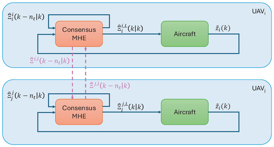
Figure 1.
Graphical representation of the communication flow between UAVs during consensus.
3.2. Local MHE
Consider a sliding window spanning time steps into the past. The measurements acquired by the i-th UAV within this sliding window are given by
At each time step k, for each consensus iteration l, with , a local constrained optimization problem is solved to compute an estimate of the state vector , denoted as .
Given a local function , defined as
with three main components:
- State dynamics: the first term addresses the state dynamics, weighted by a positive semi-definite matrix .
- Measurement-model consistency: the second term accounts for the discrepancy between the measured data and the model output, weighted by a positive definite matrix , which corresponds to the inverse of the measurement noise covariance.
- Arrival cost: the third term penalizes the error between the estimated state and the prediction , weighted by a suitable positive definite matrix , contributing to the arrival cost [50,52,69,70].
The optimization problem is defined as follows:
subject to the following constraints:
where the matrix is obtained by extracting the rows and columns corresponding to the local state from the global state matrix , whereas is the block matrix of relative to the state vector and the input vector . indicates the pseudoinverse matrix of .
Dynamics constraints (25) define the dynamics of a priori predicted state in the time window .
The initial condition (26) is obtained by selecting the suitable components of the solution at time step , after completing the consensus iterations, as .
Inequality constraints (27) restrict the possible locations of the targets to be within the sensor range .
The optimization problem represents a quadratic programming (QP) problem with linear constraints, which can be solved efficiently using well-established numerical solvers [71].
3.3. Consensus Iteration
After solving the problem defined in Section 3.2, each vehicle computes an updated estimate of the global state vector as follows:
Vehicle i exchanges its vector with the neighbors according to the consensus paradigm [72], to achieve the agreement on the global state estimation across all UAVs:
The final estimate of the global state is obtained at the end of the consensus iterations as follows:
The proposed algorithm is detailed in pseudocode in Algorithm 1 and depicted in Figure 2.
| Algorithm 1: Decentralized Moving Horizon Estimator (DMHE) |
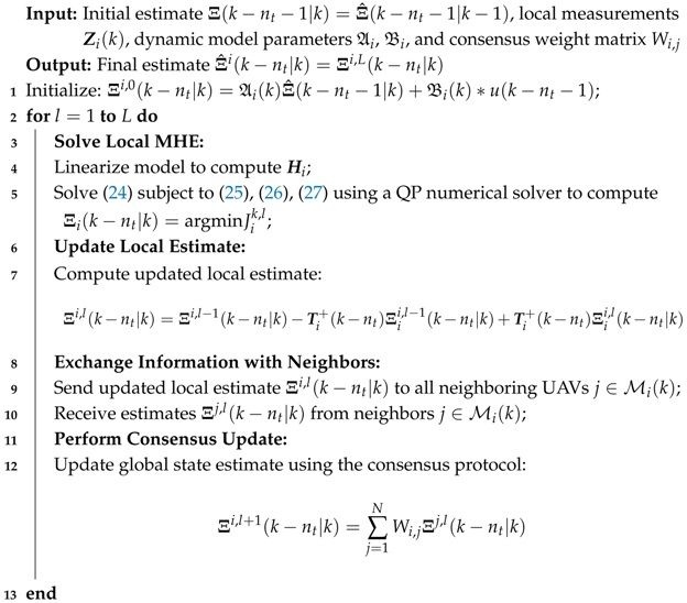 |
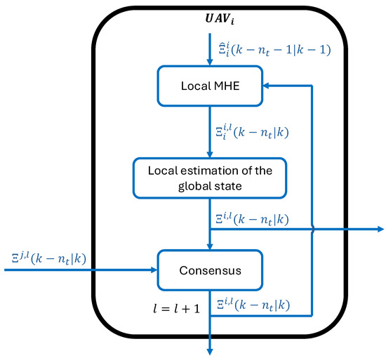
Figure 2.
Graphical representation of the DMHE flow for the i-th UAV.
4. Results
In this section, four distinct test cases are illustrated, to evaluate the performance of the proposed algorithm. They involve a swarm of UAVs operating over a designated area of interest.
The first test case was designed to carry out a sensitivity analysis, aiming to investigate how variations in key parameters, such as the number of consensus iterations (L), the number of receding iterations (), and different communication link schemes (), affect the algorithm behavior.
The objective of the second test case was to assess the performance of the algorithm in the presence of communication faults, by analyzing the effects of two distinct communication interruptions among the collaborative agents.
Test cases #3 and #4 were designed to evaluate the performance of the algorithm in estimating the position and the speed of a non-collaborative target.
The numerical simulations were carried out in a Matlab environment, considering a simulation period of s. In every test, at the beginning of the simulation, each aircraft initializes its global state estimate with random values. This assumption was useful for assessing the convergence of the algorithm toward an accurate estimate and its ability to achieve consensus.
Each simulation considers white Gaussian noise affecting GPS and the transponder, as summarized in Table 1.

Table 1.
Sensor biases and measurement noise covariance matrices considered in the simulations.
To assess the performance of the proposed algorithm, two indicators were defined: the standard deviation (SD) and the average error [73]. Assuming that indicates the position of the j-th agent estimated by the aircraft i, the estimation error at time instant k is given by
The average error in a time window composed by time steps is
Similarly, it is possible to define the standard deviation with respect to the average error as follows:
4.1. Test Case #1
This subsection shows the results of a sensitivity analysis conducted considering a scenario involving a formation of nine quadrotor UAVs, with eight agents flying in the same direction at a constant speed of 2 m/s, while UAV #1 serves as a communication base for the rest of the swarm, remaining in hovering at a fixed point in the operational scenario. During the flight, drones perform several maneuvers, both in the horizontal and the vertical plane, changing the altitude of the drones of the swarm, to assess the quality of the estimates even during dynamic phases. Table 2 summarizes the initial position of each drone of the swarm.
Table 2.
UAVs starting positions.
This first test case is useful for evaluating how the operational parameters, such as the communication link schemes, the number of consensus steps, and the number of horizon steps, influence the performance of the proposed algorithm.
The sensitivity analysis considers four configurations for the number of consensus steps (), three configurations for the number of receding steps (), and two communication schemes (, ), characterized by an increasing number of communication links, as illustrated in Figure 3.
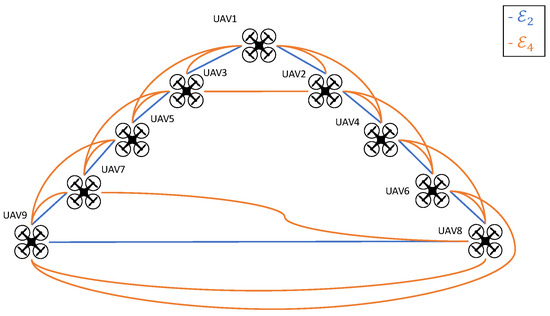
Figure 3.
Test case #1: Communication schemes among the drones. In , each aircraft communicates with two neighbors; in , each aircraft communicates with four neighbors.
The results of the numerical simulations, in terms of the estimation error made by UAV #1 in estimating the trajectory of UAV #2, are presented in Figure 4. Each figure corresponds to a different moving time horizon (, , and ) and shows error bars that represent the average error and the standard deviation for each communication scheme and number of consensus steps L.
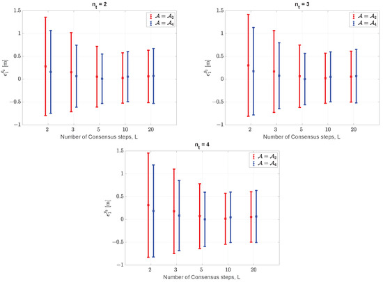
Figure 4.
Test case #1: Graphical comparison of the estimation error made by UAV #1 in estimating the position of UAV #2 as a function of the consensus steps (L) and the communication link schemes () with . The middle point of each bar represents the average error, , while the endpoints correspond to the minimum and maximum values of the standard deviation .
It is worth noting that increasing the size of the moving time horizon does not significantly impact performance, which is already satisfactory for , given the same controller tuning parameters. At the same time, as expected, the communication scheme requires a higher number of communication steps. However, beyond , further improvements in the estimates become negligible.
To choose the best configuration trade-off, an evaluation of the computational load on the CPU is needed. Figure 5 shows the computation time per estimation step for all the previously discussed configurations, varying the estimation window size () and the number of consensus steps (L). From the analysis of the figures, the configuration with and emerges as the optimal trade-off. This choice ensures a low estimation error while maintaining a reasonable computational cost, with the CPU load peaking at under a sampling time of 1 s. The results presented in the following sections were obtained using such optimal configuration.
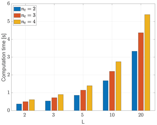
Figure 5.
Test case #1: Graphical comparison of the DMHE computation time per estimation step, varying the estimation window size () and the number of consensus steps (L). The numerical simulations were performed on a laptop equipped with an Apple M3 processor and 16 GB of RAM.
As a representative example, Figure 6 illustrates the estimated trajectories of UAV #1, UAV #2, and UAV #9 as observed from UAV #1, alongside their actual trajectories. It is worth noting that, under the communication scheme, only UAV #2 and UAV #3 communicate directly with UAV #1, as depicted in Figure 3. Nevertheless, UAV #1 successfully estimates the trajectories of both the visible UAV (UAV #2) and the non-visible UAV (UAV #9), achieving a limited estimation error, even in the presence of maneuvers. The scenario includes left and right turning maneuvers in the horizontal plane at s and s, followed by pull-up and pull-down maneuvers in the vertical plane at s and s, each lasting 20 s.
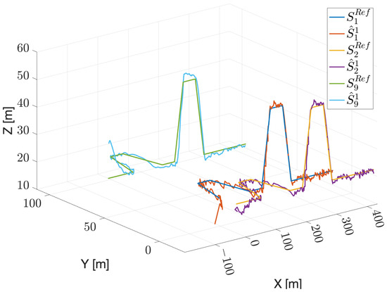
Figure 6.
Test case #1: Estimated trajectories of UAV #1, UAV #2, and UAV #9 made by UAV #1, considering , consensus steps and a moving horizon with .
4.2. Test Case #2
The following test case considers the same initial formation configuration used in test case #1 (see Table 2). Here, all UAVs fly along the same direction at a constant speed of 2 m/s, performing a series of maneuvers in the horizontal plane before reaching the destination point, as highlighted in Figure 7.
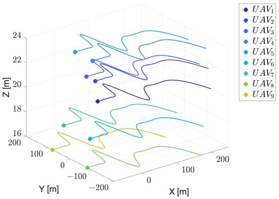
Figure 7.
Test case #2: UAVs reference trajectories.
The primary objective of this test case was to evaluate the ability of the proposed algorithm to recover the estimation of the UAVs trajectories following interruptions in the inter-agents communication. In particular, to emphasize this aspect, this scenario introduces communication link failures between UAVs during flight due to obstacle avoidance at two specific time intervals: the first at s and the second at s, both with a duration of s. Figure 8 depicts the communication link scheme during the communication interruption. In particular, when data transmission between UAV #4 and UAV #6, and between UAV #5 and UAV #7 is interrupted, the two subformations are reorganized into two distinct cycle graphs.
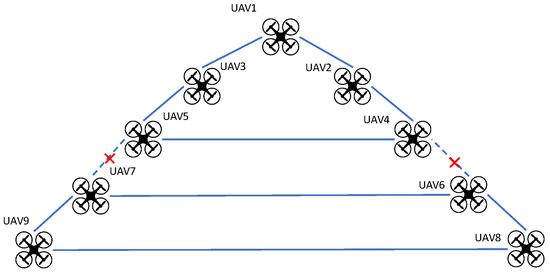
Figure 8.
Test case #2: Communication link scheme during the interruption in the data transmission between UAV #4 and UAV #6 and between UAV #5 and UAV #7.
Figure 9 shows the estimated coordinates of UAV #8 as computed by UAV #1, compared with the actual trajectory. The estimation error increases during the two designated communication interruptions and effectively decreases once the communication link is restored.
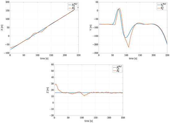
Figure 9.
Test case #2: Comparison between the estimated X,Y,Z coordinates of UAV #8 and its actual coordinates.
4.3. Test Case #3
Test case #3 was designed to assess the ability of the proposed algorithm to estimate the position of a fixed target placed at m in the operational scenario. Here, a formation of nine UAVs is considered, with eight UAVs that fly along the same direction at a constant speed of 5 m/s, with different altitudes above the terrain (see Table 2), while UAV #1 is in hovering at a fixed point, serving as a communication base. Every agent can communicate with its neighbors to form a cycle graph, as depicted in Figure 10, and it is equipped with a further transponder to detect the presence of the fixed target.
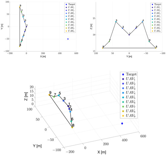
Figure 10.
Test case #3: Starting position of the UAVs and target. The solid black lines represent the communication link between aircraft.
Table 3 includes information about the bias and noise covariance of the additional transponder [63].
Table 3.
Test case #3: Bias and noise covariance of the additional transponder.
Figure 11 shows the estimation error of the coordinates of the target, comparing the actual value and the estimates made by UAV #1. Starting from random initial values, the estimation converges to the actual value in less than 10 s. The presence of a limited estimation error is further confirmed by the analysis of Table 4, which shows the average error and the standard deviation of the estimated position.
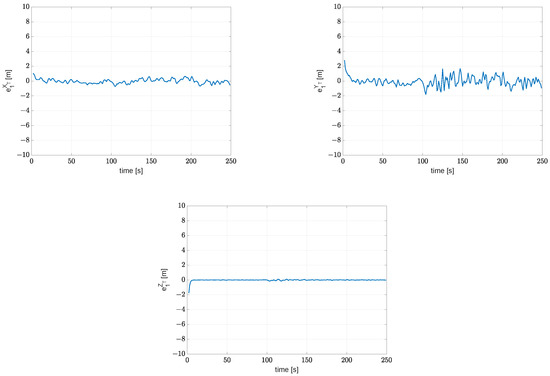
Figure 11.
Test case #3: Estimation error of target coordinates , , and as computed by UAV #1.
Table 4.
Test case #3: Estimation error of the target position. The mean value, , and the standard deviation, , are evaluated in the time window 30 s 180 s.
4.4. Test Case #4
The main aim of test case #4 was to assess the ability of the algorithm to estimate the position of a moving target, initially placed at m and moving with a velocity vector m/s. The formation is composed of nine UAVs and the initial positions of the agents of the swarm are resumed in Table 2.
Figure 12 depicts the estimation error of the target coordinates as computed by UAV #1. As shown, the estimation converges to the actual value in less than 10 s. However, as shown in Figure 12b, the estimation error grows during the first 100 s and then drops below one meter once the formation moves directly above the target. This behavior is also evident in Table 5, which reports the average error and the standard deviation of the error made by UAV #1 in the estimation of the target trajectory.
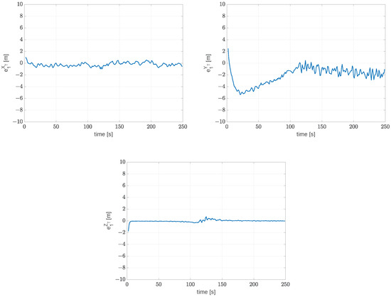
Figure 12.
Test case #4: Estimation error of target coordinates , , and as computed by UAV #1.
Table 5.
Test case #4: Estimation error of the target position. The standard deviation, , and the standard deviation, , are evaluated in the time window 150 s 200 s.
5. Conclusions
This study presented the results of the development of a DMHE for a formation of UAVs, combining consensus theory and receding horizon estimation techniques. The primary objective was to distribute computational workload across a network of UAVs while minimizing network connectivity requirements. The DMHE was designed to overcome the limitations of traditional Kalman filtering. Additionally, the algorithm was tailored to facilitate the identification of a target position, providing robust situational awareness within a distributed UAV swarm.
The results proved the algorithm’s ability to achieve consensus on the positions of both the UAVs and the target, even under challenging conditions such as communication interruptions. Several tests were carried out to evaluate the performance of the algorithm. A sensitivity analysis of the main configuration parameters showed the ability of the DMHE to successfully estimate the trajectories of UAVs, despite limited communication links, using several configurations in terms of consensus steps and receding horizon size. The results highlight the configuration and as an optimal trade-off, balancing estimation accuracy and computational cost.
The DMHE represents an interesting solution for distributed estimation in UAV swarms, offering reliable performance and robustness to communication faults. Its integration into real-world applications could enhance situational awareness and coordination in autonomous systems.
Author Contributions
Conceptualization, S.R.B., E.D. and I.N.; data curation, S.R.B. and I.N.; formal analysis, S.R.B., E.D. and I.N.; investigation, S.R.B., E.D. and I.N.; methodology, S.R.B., E.D. and I.N.; software, S.R.B., E.D. and I.N.; supervision, E.D.; validation, S.R.B., E.D. and I.N.; writing—original draft, S.R.B., E.D. and I.N.; writing—review and editing, S.R.B., E.D. and I.N. All authors have read and agreed to the published version of the manuscript.
Funding
This work was supported by the research project—ID:P2022XER7W “CHEMSYS: Cooperative Heterogeneous Multi-drone SYStem for disaster prevention and first response” granted by the Italian Ministry of University and Research (MUR) within the PRIN 2022 PNRR program, funded by the European Union through the PNRR program.
Institutional Review Board Statement
Not applicable.
Informed Consent Statement
Not applicable.
Data Availability Statement
The data presented in this study are available on request from the authors.
Conflicts of Interest
The authors declare no conflicts of interest.
Abbreviations
The following abbreviations are used in this manuscript:
| AHRS | Attitude and Heading Reference System |
| AOA | Angle of Arrival |
| CPU | Central Processing Unit |
| DKF | Decentralized Kalman Filter |
| DMHE | Distributed Moving Horizon Estimation |
| EKF | Extended Kalman Filter |
| GPS | Global Positioning System |
| HCMCI-KF | Hybrid Consensus on Measurements and Consensus on Information Kalman Filter |
| INS | Insertial Navigation System |
| IoT | Internet of Things |
| KF | Kalman Filter |
| KCF | Kalman Consensus Filter |
| MHE | Moving Horizon Estimation |
| MLE | Maximum Likelihood Estimation |
| MPC | Model Predictive Control |
| MTS | Multi Time Scale |
| NCV | Nearly Constant Velocity |
| NED | North East Down |
| RSS | Received Signal Strength |
| SD | Standard Deviation |
| STS | Single Time Scale |
| ToA | Time of Arrival |
| ToF | Time of Flight |
| UAV | Unmanned Aerial Vehicle |
References
- Mohsan, S.A.H.; Khan, M.A.; Noor, F.; Ullah, I.; Alsharif, M.H. Towards the unmanned aerial vehicles (UAVs): A comprehensive review. Drones 2022, 6, 147. [Google Scholar] [CrossRef]
- Phadke, A.; Medrano, F.A. Increasing Operational Resiliency of UAV Swarms: An Agent-Focused Search and Rescue Framework. Aerosp. Res. Commun. 2024, 1, 12420. [Google Scholar] [CrossRef]
- Lee, W.; Kim, D. Autonomous shepherding behaviors of multiple target steering robots. Sensors 2017, 17, 2729. [Google Scholar] [CrossRef]
- Sun, F.; Turkoglu, K. Distributed real-time non-linear receding horizon control methodology for multi-agent consensus problems. Aerosp. Sci. Technol. 2017, 63, 82–90. [Google Scholar] [CrossRef]
- Guo, X.; Lu, J.; Alsaedi, A.; Alsaadi, F.E. Bipartite consensus for multi-agent systems with antagonistic interactions and communication delays. Phys. A Stat. Mech. Its Appl. 2018, 495, 488–497. [Google Scholar] [CrossRef]
- Bassolillo, S.R.; D’Amato, E.; Notaro, I.; Blasi, L.; Mattei, M. Decentralized mesh-based model predictive control for swarms of UAVs. Sensors 2020, 20, 4324. [Google Scholar] [CrossRef] [PubMed]
- Simonetto, A.; Keviczky, T.; Babuška, R. Distributed nonlinear estimation for robot localization using weighted consensus. In Proceedings of the 2010 IEEE International Conference on Robotics and Automation, Anchorage, Alaska, 3–8 May 2010; pp. 3026–3031. [Google Scholar]
- Mitchell, H.B. Multi-Sensor Data Fusion: An Introduction; Springer Science & Business Media: Berlin/Heidelberg, Germany, 2007. [Google Scholar]
- Su, K.; Qian, F. Multi-UAV Cooperative Searching and Tracking for Moving Targets Based on Multi-Agent Reinforcement Learning. Appl. Sci. 2023, 13, 11905. [Google Scholar] [CrossRef]
- Xia, Z.; Du, J.; Wang, J.; Jiang, C.; Ren, Y.; Li, G.; Han, Z. Multi-agent reinforcement learning aided intelligent UAV swarm for target tracking. IEEE Trans. Veh. Technol. 2021, 71, 931–945. [Google Scholar] [CrossRef]
- Olfati-Saber, R.; Jalalkamali, P. Collaborative target tracking using distributed Kalman filtering on mobile sensor networks. In Proceedings of the 2011 American Control Conference, San Francisco, CA, USA, 29 June–1 July 2011; pp. 1100–1105. [Google Scholar]
- Li, X.R.; Jilkov, V.P. Survey of maneuvering target tracking. Part I. Dynamic models. IEEE Trans. Aerosp. Electron. Syst. 2003, 39, 1333–1364. [Google Scholar]
- Deghat, M.; Shames, I.; Anderson, B.D.; Yu, C. Localization and circumnavigation of a slowly moving target using bearing measurements. IEEE Trans. Autom. Control 2014, 59, 2182–2188. [Google Scholar] [CrossRef]
- Olfati-Saber, R.; Sandell, N.F. Distributed tracking in sensor networks with limited sensing range. In Proceedings of the 2008 American Control Conference, Seattle, WA, USA, 11–13 June 2008; pp. 3157–3162. [Google Scholar]
- Orton, M.; Fitzgerald, W. A Bayesian approach to tracking multiple targets using sensor arrays and particle filters. IEEE Trans. Signal Process. 2002, 50, 216–223. [Google Scholar] [CrossRef]
- Singh, J.; Madhow, U.; Kumar, R.; Suri, S.; Cagley, R. Tracking multiple targets using binary proximity sensors. In Proceedings of the 6th International Conference on Information Processing in Sensor Networks, Cambridge, MA, USA, 25–27 April 2007; pp. 529–538. [Google Scholar]
- Khan, M.; Heurtefeux, K.; Mohamed, A.; Harras, K.A.; Hassan, M.M. Mobile target coverage and tracking on drone-be-gone UAV cyber-physical testbed. IEEE Syst. J. 2017, 12, 3485–3496. [Google Scholar] [CrossRef]
- Ham, A. Drone-based material transfer system in a robotic mobile fulfillment center. IEEE Trans. Autom. Sci. Eng. 2019, 17, 957–965. [Google Scholar] [CrossRef]
- Benevento, A.; Santos, M.; Notarstefano, G.; Paynabar, K.; Bloch, M.; Egerstedt, M. Multi-robot coordination for estimation and coverage of unknown spatial fields. In Proceedings of the 2020 IEEE International Conference on Robotics and Automation (ICRA), Paris, France, 31 May–31 August 2020; pp. 7740–7746. [Google Scholar]
- Chen, Q.; Sun, Y.; Zhao, M.; Liu, M. Consensus-based cooperative formation guidance strategy for multiparafoil airdrop systems. IEEE Trans. Autom. Sci. Eng. 2020, 18, 2175–2184. [Google Scholar] [CrossRef]
- Shafiei, M.; Vazirpour, N. The approach of partial stabilisation in design of discrete-time robust guidance laws against manoeuvering targets. Aeronaut. J. 2020, 124, 1114–1127. [Google Scholar] [CrossRef]
- Taghieh, A.; Shafiei, M.H. Observer-based robust model predictive control of switched nonlinear systems with time delay and parametric uncertainties. J. Vib. Control 2021, 27, 1939–1955. [Google Scholar] [CrossRef]
- Koivisto, M.; Hakkarainen, A.; Costa, M.; Talvitie, J.; Heiska, K.; Leppänen, K.; Valkama, M. Continuous high-accuracy radio positioning of cars in ultra-dense 5G networks. In Proceedings of the 2017 13th International Wireless Communications and Mobile Computing Conference (IWCMC), Valencia, Spain, 26–30 June 2017; pp. 115–120. [Google Scholar]
- Haber, A.; Molnar, F.; Motter, A.E. State observation and sensor selection for nonlinear networks. IEEE Trans. Control Netw. Syst. 2017, 5, 694–708. [Google Scholar] [CrossRef]
- Zhao, Z.; Li, T.R.; Jilkov, V.P. Best linear unbiased filtering with nonlinear measurements for target tracking. IEEE Trans. Aerosp. Electron. Syst. 2004, 40, 1324–1336. [Google Scholar] [CrossRef]
- He, D.; Qiao, Y.; Chan, S.; Guizani, N. Flight security and safety of drones in airborne fog computing systems. IEEE Commun. Mag. 2018, 56, 66–71. [Google Scholar] [CrossRef]
- Kehoe, B.; Patil, S.; Abbeel, P.; Goldberg, K. A survey of research on cloud robotics and automation. IEEE Trans. Autom. Sci. Eng. 2015, 12, 398–409. [Google Scholar] [CrossRef]
- Chen, W.; Liu, J.; Guo, H. Achieving robust and efficient consensus for large-scale drone swarm. IEEE Trans. Veh. Technol. 2020, 69, 15867–15879. [Google Scholar] [CrossRef]
- Abdelmawgoud, A.; Pack, D.; Ruble, Z. Consensus-based distributed estimation in multi-agent systems with time delay. In Proceedings of the 2018 World Automation Congress (WAC), Stevenson, WA, USA, 3–6 June 2018; pp. 1–5. [Google Scholar]
- DeGroot, M.H. Reaching a consensus. J. Am. Stat. Assoc. 1974, 69, 118–121. [Google Scholar] [CrossRef]
- Olfati-Saber, R.; Murray, R.M. Consensus problems in networks of agents with switching topology and time-delays. IEEE Trans. Autom. Control 2004, 49, 1520–1533. [Google Scholar] [CrossRef]
- Olfati-Saber, R.; Fax, J.A.; Murray, R.M. Consensus and cooperation in networked multi-agent systems. Proc. IEEE 2007, 95, 215–233. [Google Scholar] [CrossRef]
- Doostmohammadian, M. Single-bit consensus with finite-time convergence: Theory and applications. IEEE Trans. Aerosp. Electron. Syst. 2020, 56, 3332–3338. [Google Scholar] [CrossRef]
- Boukhobza, T.; Hamelin, F.; Martinez-Martinez, S.; Sauter, D. Structural analysis of the partial state and input observability for structured linear systems: Application to distributed systems. Eur. J. Control 2009, 15, 503–516. [Google Scholar] [CrossRef]
- Kar, S.; Moura, J.M.; Ramanan, K. Distributed parameter estimation in sensor networks: Nonlinear observation models and imperfect communication. IEEE Trans. Inf. Theory 2012, 58, 3575–3605. [Google Scholar] [CrossRef]
- Das, S.; Moura, J.M. Distributed Kalman filtering with dynamic observations consensus. IEEE Trans. Signal Process. 2015, 63, 4458–4473. [Google Scholar] [CrossRef]
- Zhong, X.; Mohammadi, A.; Premkumar, A.B.; Asif, A. A distributed particle filtering approach for multiple acoustic source tracking using an acoustic vector sensor network. Signal Process. 2015, 108, 589–603. [Google Scholar] [CrossRef]
- Ennasr, O.; Xing, G.; Tan, X. Distributed time-difference-of-arrival (TDOA)-based localization of a moving target. In Proceedings of the 2016 IEEE 55th Conference on Decision and Control (CDC), Las Vegas, NV, USA 12–14 December 2016; pp. 2652–2658. [Google Scholar]
- He, X.; Hu, C.; Hong, Y.; Shi, L.; Fang, H.T. Distributed Kalman filters with state equality constraints: Time-based and event-triggered communications. IEEE Trans. Autom. Control 2019, 65, 28–43. [Google Scholar] [CrossRef]
- He, X.; Ren, X.; Sandberg, H.; Johansson, K.H. How to secure distributed filters under sensor attacks. IEEE Trans. Autom. Control 2021, 67, 2843–2856. [Google Scholar] [CrossRef]
- Chen, W.; Liu, J.; Guo, H.; Kato, N. Toward robust and intelligent drone swarm: Challenges and future directions. IEEE Netw. 2020, 34, 278–283. [Google Scholar] [CrossRef]
- Bassolillo, S.R.; Blasi, L.; D’Amato, E.; Mattei, M.; Notaro, I. Decentralized Triangular Guidance Algorithms for Formations of UAVs. Drones 2022, 6, 7. [Google Scholar] [CrossRef]
- Olfati-Saber, R. Distributed Kalman filter with embedded consensus filters. In Proceedings of the 44th IEEE Conference on Decision and Control, Seville, Spain, 12–15 December 2005; pp. 8179–8184. [Google Scholar]
- Olfati-Saber, R. Kalman-consensus filter: Optimality, stability, and performance. In Proceedings of the 48h IEEE Conference on Decision and Control (CDC) held jointly with 2009 28th Chinese Control Conference, Shanghai, China, 15–18 December 2009; pp. 7036–7042. [Google Scholar]
- Zhou, Z.; Fang, H.; Hong, Y. Distributed estimation for moving target based on state-consensus strategy. IEEE Trans. Autom. Control 2013, 58, 2096–2101. [Google Scholar] [CrossRef]
- Wang, S.; Ren, W.; Li, Z. Information-driven fully distributed Kalman filter for sensor networks in presence of naive nodes. arXiv 2014, arXiv:1410.0411. [Google Scholar]
- Allgöwer, F.; Badgwell, T.A.; Qin, J.S.; Rawlings, J.B.; Wright, S.J. Nonlinear predictive control and moving horizon estimation—An introductory overview. In Advances in Control; Springer: London, UK, 1999; pp. 391–449. [Google Scholar]
- Franze, G.; Mattei, M.; Ollio, L.; Scordamaglia, V. A robust constrained model predictive control scheme for norm-bounded uncertain systems with partial state measurements. Int. J. Robust Nonlinear Control 2019, 29, 6105–6125. [Google Scholar] [CrossRef]
- Allan, D.A.; Rawlings, J.B. Moving horizon estimation. In Handbook of Model Predictive Control; Springer International Publishing: Cham, Germany, 2019; pp. 99–124. [Google Scholar]
- Rao, C.V.; Rawlings, J.B.; Lee, J.H. Constrained linear state estimation—A moving horizon approach. Automatica 2001, 37, 1619–1628. [Google Scholar] [CrossRef]
- Alessandri, A.; Baglietto, M.; Battistelli, G. Receding-horizon estimation for discrete-time linear systems. IEEE Trans. Autom. Control 2003, 48, 473–478. [Google Scholar] [CrossRef]
- Alessandri, A.; Baglietto, M.; Battistelli, G. Moving-horizon state estimation for nonlinear discrete-time systems: New stability results and approximation schemes. Automatica 2008, 44, 1753–1765. [Google Scholar] [CrossRef]
- Ferrari-Trecate, G.; Mignone, D.; Morari, M. Moving horizon estimation for hybrid systems. IEEE Trans. Autom. Control 2002, 47, 1663–1676. [Google Scholar] [CrossRef]
- Farina, M.; Ferrari-Trecate, G.; Scattolini, R. Distributed moving horizon estimation for linear constrained systems. IEEE Trans. Autom. Control 2010, 55, 2462–2475. [Google Scholar] [CrossRef]
- Farina, M.; Ferrari-Trecate, G.; Scattolini, R. Distributed moving horizon estimation for nonlinear constrained systems. Int. J. Robust Nonlinear Control 2012, 22, 123–143. [Google Scholar] [CrossRef]
- Battistelli, G. Distributed moving-horizon estimation with arrival-cost consensus. IEEE Trans. Autom. Control 2018, 64, 3316–3323. [Google Scholar] [CrossRef]
- Huang, Z.; Lv, W.; Liu, C.; Xu, Y.; Rutkowski, L.; Huang, T. Event-triggered distributed moving horizon estimation over wireless sensor networks. IEEE Trans. Ind. Inform. 2024, 20, 4218–4226. [Google Scholar] [CrossRef]
- Yu, D.; Xia, Y.; Zhai, D.H. Distributed moving-horizon estimation with event-triggered communication over sensor networks. IEEE Trans. Autom. Control 2023, 68, 7982–7988. [Google Scholar] [CrossRef]
- Kim, J.; Kang, J.H.; Bae, J.; Lee, W.; Kim, K.K.K. Distributed moving horizon estimation via operator splitting for automated robust power system state estimation. IEEE Access 2021, 9, 90428–90440. [Google Scholar] [CrossRef]
- Zou, L.; Wang, Z.; Shen, B.; Dong, H. Moving horizon estimation over relay channels: Dealing with packet losses. Automatica 2023, 155, 111079. [Google Scholar] [CrossRef]
- Rajab, K.Z.; Wu, B.; Alizadeh, P.; Alomainy, A. Multi-target tracking and activity classification with millimeter-wave radar. Appl. Phys. Lett. 2021, 119, 034101. [Google Scholar] [CrossRef]
- Yeste-Ojeda, O.A.; Zambrano, J.; Landry, R. Design of integrated Mode S transponder, ADS-B and distance measuring equipment transceivers. In Proceedings of the 2016 Integrated Communications Navigation and Surveillance (ICNS), Herndon, VA, USA, 19–21 April 2016; pp. 4E1–4E8. [Google Scholar]
- Bassolillo, S.R.; D’Amato, E.; Mattei, M.; Notaro, I. Distributed navigation in emergency scenarios: A case study on post-avalanche search and rescue using drones. Appl. Sci. 2023, 13, 11186. [Google Scholar] [CrossRef]
- Dogru, S.; Marques, L. Pursuing drones with drones using millimeter wave radar. IEEE Robot. Autom. Lett. 2020, 5, 4156–4163. [Google Scholar] [CrossRef]
- Hansard, M.; Lee, S.; Choi, O.; Horaud, R.P. Time-of-Flight Cameras: Principles, Methods and Applications; Springer Science & Business Media: Berlin/Heidelberg, Germany, 2012. [Google Scholar]
- Kühl, P.; Diehl, M.; Kraus, T.; Schlöder, J.P.; Bock, H.G. A real-time algorithm for moving horizon state and parameter estimation. Comput. Chem. Eng. 2011, 35, 71–83. [Google Scholar] [CrossRef]
- Saber, R.O.; Murray, R.M. Consensus protocols for networks of dynamic agents. In Proceedings of the 2003 American Control Conference, Denver, CO, USA, 4–6 June 2003; Volume 2, pp. 951–956. [Google Scholar]
- Xiao, L.; Boyd, S.; Lall, S. A scheme for robust distributed sensor fusion based on average consensus. In Proceedings of the IPSN 2005 Fourth International Symposium on Information Processing in Sensor Networks, Los Angeles, CA, USA, 25–27 April 2005; pp. 63–70. [Google Scholar]
- Muske, K.R.; Rawlings, J.B.; Lee, J.H. Receding horizon recursive state estimation. In Proceedings of the 1993 American Control Conference, San Antonio, TX, USA, 9–12 May 1993; pp. 900–904. [Google Scholar]
- Alessandri, A.; Baglietto, M.; Battistelli, G.; Zavala, V. Advances in moving horizon estimation for nonlinear systems. In Proceedings of the 49th IEEE Conference on Decision and Control (CDC), Atlanta, GA, USA, 15–17 December 2010; pp. 5681–5688. [Google Scholar]
- Nocedal, J.; Wright, S.J. Numerical Optimization; Springer: New York, NY, USA, 1999. [Google Scholar]
- Battistelli, G.; Chisci, L. Stability of consensus extended Kalman filter for distributed state estimation. Automatica 2016, 68, 169–178. [Google Scholar] [CrossRef]
- Willmott, C.J.; Matsuura, K. Advantages of the mean absolute error (MAE) over the root mean square error (RMSE) in assessing average model performance. Clim. Res. 2005, 30, 79–82. [Google Scholar] [CrossRef]
Disclaimer/Publisher’s Note: The statements, opinions and data contained in all publications are solely those of the individual author(s) and contributor(s) and not of MDPI and/or the editor(s). MDPI and/or the editor(s) disclaim responsibility for any injury to people or property resulting from any ideas, methods, instructions or products referred to in the content. |
© 2025 by the authors. Licensee MDPI, Basel, Switzerland. This article is an open access article distributed under the terms and conditions of the Creative Commons Attribution (CC BY) license (https://creativecommons.org/licenses/by/4.0/).