Hierarchical Online Air Combat Maneuver Decision Making and Control Based on Surrogate-Assisted Differential Evolution Algorithm

Abstract

One-to-one within-visual-range air combat of unmanned combat aerial vehicles (UCAVs) requires fast, continuous, and accurate decision-making to achieve air combat victory. In order to solve the current problems of insufficient real-time performance of traditional intelligent optimization algorithms for solving decision-making problems and the mismatch between the planning trajectory and the actual flight trajectory caused by the difference between the decision-making model and the actual aircraft model, this paper proposes a hierarchical on-line air combat maneuvering decision-making and control framework. Considering the real-time constraints, the maneuver decision problem is transformed into an expensive optimization problem at the decision planning layer. The surrogate-assisted differential evolution algorithm is proposed on the basis of the original differential evolution algorithm, and the planning trajectory is obtained through the 5 degrees of freedom (DOF) model. In the control execution layer, the planning trajectory is tracked through the nonlinear dynamic inverse tracking control method to realize the high-precision control of the 6DOF model. The simulation is carried out under four different initial situation scenarios, including head-on neutral, dominant, parallel neutral, and disadvantaged situations. The Monte Carlo simulation results show that the Surrogate-assisted differential evolution algorithm (SADE) can achieve a win rate of over 53% in all four initial scenarios. The proposed maneuver decision and control framework in this article achieves smooth flight trajectories and stable aircraft control, with each decision average taking 0.08 s, effectively solving the real-time problem of intelligent optimization algorithms in maneuver decision problems.

1. Introduction

With the development of modern warfare towards unmanned and intelligent combat, unmanned combat aerial vehicles (UCAVs) have gradually become an important combat force on the battlefield. UCAVs are characterized by high performance, low cost ratio, and low risk, and are therefore widely used in battlefield reconnaissance [1], risk assessment [2], and aerial refueling [3]. With the rapid improvement in sensor technology and computing capacity, the autonomous decision-making capability of air combat systems has been gradually improved [4], and some projects and studies are already underway, although fully autonomous air combat systems have not yet been realized.

As the core of autonomous air combat system, maneuver decision-making is a challenging task, and many scholars are currently trying to solve this problem by using traditional methods or new intelligent methods. There are three main current autonomous air combat maneuver decision-making methods, including game theory-based methods [5,6], self-learning-based methods [7,8,9,10,11], and optimization theory-based methods [12,13,14,15].

Game theory has been widely used in military confrontation and is also an effective method for solving air combat game problems. The methods based on game theory mainly include differential game methods and influence diagram methods. Lee et al. [5] discretizes the continuous air combat game problem and constructs the payment matrices of the two sides of the game at each time step for evaluating the decisions; then it solves the equilibrium decisions in the decision sets of the two sides by using the principle of great and small values. The method is mainly limited by the number of maneuvers and the lack of continuity due to the discrete decision variables. Virtanen et al. [6] proposes a multilevel influence diagram game model, which uses the moving horizon control method to solve the influence diagram game and obtains the optimal control sequences of the pilots with respect to their preference models, but the method is subject to a large subjective influence.

Self-learning based methods mainly include Bayesian inference methods, approximate dynamic programming methods, neural network methods, and deep reinforcement learning methods. Huang et al. [7] regards air combat confrontation as a Markov process. By constructing a dynamic Bayesian network using Bayesian optimization methods, it adaptively adjusts the weights of the maneuver decision factors to make the objective function more reasonable and ensure the superior posture of the unmanned aircraft. The method proposed by C.Q. Huang mainly considers the prior knowledge of domain experts and pilots, and the performance of its model is greatly affected by subjective factors. Moreover, in more complex aerial combat scenarios, the Bayesian inference based maneuver decision model is likely to has insufficient adaptability. J.B. Crumpacker et al. [8] constructs a neural network-based approximate dynamic planning (ADP) algorithm to generate high-quality UCAV maneuvering strategies. The experimental results show that the maneuvering strategy obtained by solving based on the ADP method outperforms the baseline strategy that only considers the position and the baseline strategy that considers both the position and energy, as the ADP method is more efficient in managing the kinetic and potential energy of the AUCAV. However, the neural network used in this method is not deep enough, and the maneuver decision model is less generalizable. When facing confrontation scenarios that are different from the model training phase, the optimal action strategy obtained by solving the maneuver decision model tends to perform poorly in the confrontation effect. Zhang and Huang [9] proposed a deep learning method for air combat maneuver decision-making. The fatal problem with the deep learning method is that relying solely on deep learning cannot encourage agents to explore new strategies and respond in unfamiliar situations. Agents can only respond to the following situations in training samples or similar events [16]. In addition, due to the huge state space for both aircraft during air combat, which reached 25 dimensions in the reference [17], it is difficult to obtain samples that cover the full states. Deep reinforcement learning-based maneuver decision-making methods have been widely studied in recent years. Li et al. [10] proposes to use the MS-DDQN algorithm for air combat maneuver decision-making and designs the controller of a 6DOF vehicle at the bottom layer for tracking the commands derived from the decision-making, but the action space of the method is not continuous and the flight trajectory obtained is obviously not smooth enough. In order to solve the problem of neural network plasticity loss in traditional course learning, a Motivated Course Learning Distributed Proximal Policy Optimization (MCLDPPO) algorithm is proposed in [11], by which the trained intelligences can significantly outperform the predictive game tree and mainstream reinforcement learning methods. However, the feasibility of the designed maneuver types under different state conditions was not considered in the paper. The H3E hierarchical maneuver decision framework was proposed in [18], and simulation results show that agents using control surface deflection as the action space without controllers have difficulty obtaining game strategies when learning maneuver actions, resulting in few effective strategies being learned. In [19], it is pointed out that the algorithm directly outputs the control surface deflection, which makes it difficult to control the smooth flight of the aircraft and is not conducive to the training of intelligent agents. It is also difficult for intelligent agents to learn effective air combat strategies. Overall, the decision output of deep reinforcement learning methods often cannot directly use the control surface deflection as the action space (this is because agents need to learn flight control while learning air combat confrontation), but, rather, the basic maneuvers are used as the action space for deep reinforcement learning through hierarchization. However, whether the basic maneuvers can be effectively executed under the current flight state is not taken into account, and since the deep reinforcement learning method is a black-box with non-interpretability, the decision reliability needs to be further considered.

Intelligent optimization-based methods mainly use intelligent optimization algorithms for air combat maneuver decision-making. Duan et al. [12] uses the game hybrid strategy to design the objective function and obtains the optimal hybrid strategy using an improved pigeon-inspired optimization algorithm, which has been proven to be superior to the min–max search algorithm and the remaining several classical optimization algorithms in simulations. Ernest et al. [13] proposed a GA-based fuzzy inference system known as ALPHA. In the air combat simulation, ALPHA successfully defeated two jet fighters operated by retired fighter pilots. However, the rules established for specific missions cannot be transplanted into new task, and the trees optimized using genetic algorithms (GA) cannot be reconstructed with the combat result and recorded data, which hinders enrichment of expert knowledge [16]. Duan et al. [14] proposes a game theory approach based on predator–prey particle swarm optimization, where each side in every decision-making step seeks the optimal solution with the aim of maximizing its own objective function, but it requires significant computational resources, making it time-consuming and difficult to achieve real-time decision-making [20]. Ruan et al. [15] calculates the air combat posture assessment function based on angle and distance threats and composes the game matrix. Then, it designs the objective function to be optimized using the game mixing strategy and obtains the optimal mixing strategy through TLPIO. The main drawback of intelligent optimization-based approaches is their difficulty in meeting the real-time demands of air combat decision-making.

Most of the above work has been performed using a 3DOF model simplified from 6DOF models, which are far from the actual 6DOF vehicle models with complex aerodynamic forces, and thus lack practical feasibility. In papers that used a 6DOF vehicle model [10,12,15,21], they designed controllers to convert 3DOF control variables to a 6DOF model, but the control systems were all relatively simple. References [12,15] do not have control over the thrust. Reference [15] scales the normal overload obtained from the decision to an angle of attack control variable as an input, which is likely to cause the controller’s inputs to oscillate and cause tracking errors. Therefore, it is not capable of tracking the paths that were planned using 3DOF models. There is no mention in [12] of how to translate the overload obtained from the decision into the angle of attack in the control commands. The controller designed in the literature [10] tracks flight path azimuth angle, roll angle, and velocity, but the simulation does not manage to track all three variables at the same time. Reference [21] uses the change variables of speed, flight path slope angle, and flight path azimuth angle as decision variables, and then the dynamics equations are inverted to solve the variables of angle of attack, roll angle, and thrust. However, the inverse solution uses a system of equations that does not take into account the effect of lift. In fact, the inverse solution of the F-16 with a complex nonlinear aerodynamic model is difficult, which leads to the fact that the variations in the states obtained directly using deep reinforcement learning cannot guarantee a solution.

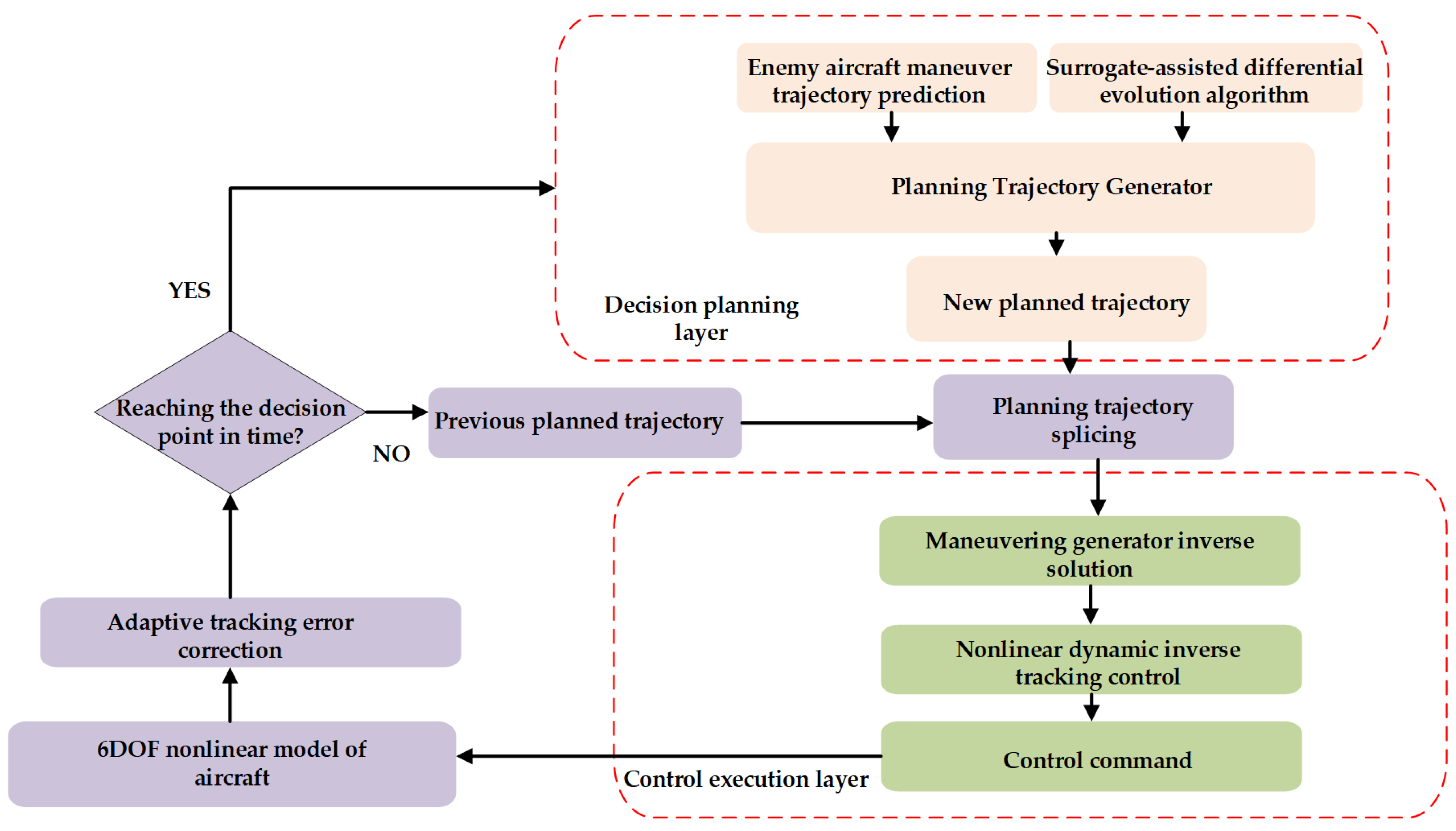
However, directly using the 6DOF model for decision-making first brings huge decision space, making it difficult to achieve good flight control effects. Secondly, it is difficult to meet real-time requirements due to the complexity of differential equations. Therefore, the 5DOF model is used in the decision planning layer and 6DOF model is used in the control execution layer in this paper. Compared to the 3DOF model, the 5DOF model uses the throttle, angle of attack, and roll angle as the control variables to solve the lift and drag force in real-time so as to generate a high-fidelity planned trajectory. The nonlinear dynamic inverse control method is used in the control execution layer to track the planned trajectory dynamically, solving the problem of the 6DOF model tracking the planned trajectory of the 5DOF model, which satisfies the high-fidelity and real-time requirements of the model at the same time.

In order to solve the problem with the intelligent optimization-based methods mentioned above, that they find it difficult to meet the real-time requirements of air combat decision-making and high-fidelity aircraft model control, this paper proposes a hierarchical online air combat maneuver decision-making and control framework. In this paper, the maneuver decision problem is transformed into an optimization problem at the decision planning layer, the optimal trajectory is planned using surrogate-assisted differential evolutionary algorithm under the real-time constraints, and the maneuver generator inverse solution is used at the control execution layer using nonlinear dynamic inverse control for tracking the planned trajectory. The main contributions of this paper are shown below:

(1) In the aircraft control layer, a 6DOF flight dynamics model of the F-16 aircraft is constructed using aerodynamic data, and a nonlinear dynamic inverse control algorithm is constructed using the MATLAB2023B/Simulink simulation platform. Aiming at the problem of high-precision tracking control of trajectories obtained by planning, the control commands are obtained using the maneuver generator inverse solution algorithm, and the comparison simulation with the PID control verifies the superiority of the nonlinear dynamic inverse algorithm in tracking the large overload maneuver.

(2) In order to solve the problem that ordinary intelligent optimization algorithms have insufficient real-time performance and cannot meet the decision-making needs, the surrogate-assisted differential evolution (SADE) algorithm is proposed on the basis of the original differential evolution algorithm. The algorithm quickly derives decision quantities within an extremely limited number of real fitness evaluations by using a radial basis function as the objective function approximation. SADE is compared with other recent variants of surrogate-assisted optimization algorithms and differential evolution algorithms on a test suite consisting of five classical benchmark problems, and the results show that the surrogate-assisted differential evolution algorithm significantly outperforms the other algorithms.

(3) In the decision planning layer, in order to obtain a high-quality planning trajectory within the aerodynamic constraints, combined with the prediction of the adversary aircraft trajectory, an objective function and a planning trajectory generator are proposed to transform the maneuver decision problem into an optimization problem. Meanwhile, in order to overcome the problem of trajectory tracking control error accumulation, adaptive tracking error correction is proposed. The SADE algorithm is confronted with other algorithms in head-on neutral, dominant, parallel neutral, and disadvantaged postures, and the results show that the SADE algorithm can all effectively drive the UCAV to obtain the air combat victory and can effectively improve the air combat victory rate compared to the traditional min–max search algorithm and random search algorithm.

The rest of this paper is organized as follows. The architecture of the autonomous maneuvering decision system is presented in Section 2. Section 3 provides a detailed description of the nonlinear dynamic inverse tracking control method in the control executive layer. Then the nonlinear dynamic inversion (NDI) method and the traditional PID tracking control method are compared in a simulation. Section 4 provides a detailed description of the surrogate-assisted differential evolutionary algorithms and planning trajectory generator used in the decision planning layer. Section 5 shows the simulation results of this paper’s SADE algorithm and several other excellent algorithms in four different initial situation scenarios. Section 6 concludes the findings of this paper.

2. Architecture of the Autonomous Maneuvering Decision System

In this paper, a hierarchical one-to-one air combat system consisting of a decision planning layer and a control execution layer is designed using an F-16 aircraft as the control object, as shown in Figure 1.

The control execution layer includes a maneuver generator inverse solution and state variable tracking for tracking the planning trajectories. This module is used to generate real pilot control commands (elevator, rudder, aileron, and throttle commands), and the input is the planning trajectory output from the decision planning layer. This module uses the maneuver generator inverse solution to obtain commands such as angle of attack and roll angle, and then generates angular velocity commands through the outer loop and control surface deflection commands through the inner loop so as to ultimately realize the trajectory tracking control.

At the decision planning layer, to plan high-quality maneuver trajectories, a 5DOF (in [8] called 5DOF model) vehicle model was used to construct a planning trajectory generator instead of a 3DOF [22] vehicle model. The decision dimension is reduced using fitting and sampling methods, and the maneuver decision problem is transformed into an optimization problem, so the mapping from decision quantities to trajectories is established. Then the situation access function is used as the objective function, the optimization problem is approximated as an expensive optimization problem in order to satisfy the real-time decision-making, and the decision variables are optimized using surrogate-assisted evolutionary algorithms to generate the planning trajectory in cases where the number of real fitness evaluations is very small.

Errors inevitably occur in the process of tracking and planning trajectories. In order to adapt to the tracking error, an adaptive tracking error correction method is introduced, which can automatically correct the tracking error. In addition, between the planning trajectory of the previous section and the planning trajectory of the next section, the planning trajectory needs to be spliced so as to make the tracker more stable.

3. Trajectory Tracking Control Method Based on Nonlinear Dynamic Inverse (Control Executive Layer)

In this section, the 6DOF aircraft is first modeled. Then the control system architecture based on the nonlinear dynamic inverse tracking control method is presented. In order to solve the planning trajectory tracking problem, the inverse solution maneuver generator is discussed in detail. Finally, the method of this paper is compared to the tracking control methods in other papers on a complex planning trajectory.

3.1. Six Degree of Freedom Aircraft Model

A 6DOF model of the airplane is used in the control layer, containing kinematics and dynamics equations [23]:

$$\begin{array}{l}\dot{x}=u\cos \theta \cos \psi +v(\sin \varphi \sin \theta \cos \psi -\cos \varphi \sin \psi )+w(\cos \varphi \sin \theta \cos \psi +\sin \varphi \sin \psi )\\ \dot{y}=u\cos \theta \sin \psi +v(\sin \varphi \sin \theta \sin \psi +\cos \varphi \cos \psi )+w(\cos \varphi \sin \theta \sin \psi -\sin \varphi \cos \psi )\\ \dot{z}=u\sin \theta -v\sin \varphi \cos \theta -w\cos \varphi \cos \theta \end{array}$$

(1)

$$\begin{array}{l}\dot{V}={\displaystyle \frac{u\dot{u}+v\dot{v}+w\dot{w}}{V}}\\ \dot{\alpha }={\displaystyle \frac{u\dot{w}-w\dot{u}}{u^2+w^2}}\\ \dot{\beta }={\displaystyle \frac{\dot{v}V-v\dot{V}}{V^2\cos \beta }}\end{array}$$

(2)

$$\begin{array}{l}\dot{p}={\displaystyle \frac{I_{xz}(I_x-I_y+I_z)pq+(I_z{I}_y-{I_z}^2-{I_{xz}}^2)qr+I_{z}L+I_{xz}N}{I_x{I}_z-{I_{xz}}^2}}\\ \dot{q}={\displaystyle \frac{M+(I_z-I_x)pr+(r^2-p^2)I_{xz}}{I_y}}\\ \dot{r}={\displaystyle \frac{I_{xz}L+I_{z}N+(I_x^2+I_z^2-I_x{I}_y)pq-I_{xz}(I_x-I_y+I_z)qr}{I_x{I}_z-I_{xz}^2}}\end{array}$$

(3)

$$\begin{array}{l}\dot{\varphi }=p+\tan \theta (r\cos \varphi +q\sin \varphi )\\ \dot{\theta }=q\cos \varphi -r\sin \varphi \\ \dot{\psi }=(r\cos \varphi +q\sin \varphi )/\cos \theta \end{array}$$

(4)

$$\begin{array}{l}\dot{u}=rv-qw-g\sin \theta +(X+T)/m;\\ \dot{v}=pw-ru+g\cos \theta \sin \varphi +Y/m;\\ \dot{w}=qu-pv+g\cos \theta \cos \varphi +Z/m;\end{array}$$

(5)

where $V,\alpha ,\beta$ are the velocity, angle of attack, and angle of sideslip, respectively. $\varphi ,\theta ,\psi$ are the roll, pitch, and yaw angles in the body coordinate system, respectively. $p,q,r$ are the angular velocity along the three axes. $u,v,w$ are the velocity components under the airplane body axis system, respectively. $x,y,z$ is the aircraft position in the ground coordinate system. The controls are $u=[{\delta }_e,{\delta }_a,{\delta }_r,{\delta }_T]$, which are elevator, aileron, rudder, and throttle. The three angles, flight path slope angle, flight path azimuth angle, and flight path roll angle, can be defined under the trajectory coordinate system as $\gamma ,\chi ,\mu$, where $\gamma \in (-\pi /2,\pi /2],\chi \in (-\pi ,\pi ],\mu \in (-\pi ,\pi ]$.

In the trajectory coordinate system, the dynamical equations can be written as follows [24]:

$$\begin{array}{l}m\dot{V}=T\cos \alpha \cos \beta -D+Y\sin \beta -mg\sin \gamma \\ mV\dot{\gamma }=T(\cos \mu \sin \alpha +\sin \mu \cos \alpha \sin \beta )+L\cos \mu -Y\sin \mu \cos \beta -mg\cos \gamma \\ mV\dot{\chi }\cos \gamma =T(\sin \mu \sin \alpha -\cos \mu \cos \alpha \sin \beta )+L\sin \mu +Y\cos \mu \cos \beta \end{array}$$

(6)

where D is drag, L is lift, and T is engine thrust.

3.2. Control System Architecture

For the 6DOF vehicle model with control surface deflection as the control variable, the trajectory roll angle and overload obtained from the three-degree-of-freedom decision are simply scaled as the angle of attack and roll angle signals for the 6DOF tracking in the literature [15], so the trajectory obtained from the actual flight may be highly different from the desired trajectory. Based on the flight path azimuth angle $\chi$, roll angle $\varphi$, and velocity V obtained in the decision-making process, [10] designed a PID controller to obtain the surface deflection control variables. The three desired commands were simulated separately, and the results show that the desired states can be reached, but the method is not described for the simultaneous control to reach the three desired states. Reference [12] designed a lateral and longitudinal autopilot based on the PID controller to track the decided angle of attack and roll angle.

There is actually a problem in all of the above papers with how the 6DOF model of the aircraft follows the flight trajectory found using the 3DOF model. It is possible that a high-quality flight path generated using the 3DOF point mass model is actually a low-quality path for the 6DOF model or that the 6DOF model cannot reasonably follow the planned flight path due to the characteristics of the 6DOF model that are not represented at lower fidelity in 3DOF (e.g., limitations on control surface rate, aerodynamics). Indeed, depending on the difference between the chosen trajectory rate limit and the trajectory rate of a particular aircraft, the 6DOF rigid body simulation may not accurately follow the prescribed trajectory. Therefore, a high-quality flight path planning algorithm and an adaptive 6DOF aircraft trajectory tracking control algorithm are solutions to this problem.

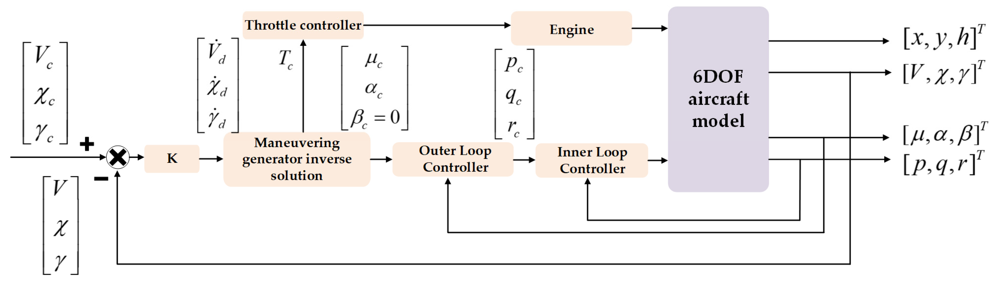
Compared to the traditional gain scheduling method, the control law of the nonlinear dynamic inverse is more accurate, the overshoot is smaller, and the required surface deflection control is smaller, which is especially obvious at large angles of attack, and avoids the complicated and tedious process of selecting state points and scheduling variables in the gain scheduling method. In order to ensure that the 6DOF model can track the planned trajectory, this paper adopts the nonlinear dynamic inverse algorithm as the control algorithm. The block diagram of the system is shown in Figure 2.

According to the timescale separation results, the aircraft state variables are grouped together and a dynamic inverse controller with cascade structure is used. According to the singular regression theory, the state variables are divided into two levels according to their speed of change. In Figure 2, $x_f={[p,q,r]}^T$ represents fast variables and $x_s={[\mu ,\alpha ,\beta ]}^T$ represents slow variables.

The fast and slow loops of the control system are the same as in [25], and will not be repeated here.

3.3. Reverse Solution of Maneuvering Generator

In trajectory planning, the dynamics equation used is Equation (6), but the angle of attack, thrust, and roll angle obtained from planning are not directly used as inputs to the control layer. The reason for this is that the calculation of lift L and drag D in the 5DOF model is different from that of the 6DOF. The values of angular velocities p, q, and r and rudder surface deflections δ_e, δ_a, and δ_r do not exist in the 5DOF model, so the calculated lift L and drag D are different, which leads to the fact that the direct use of the planned control variables as inputs to the tracking variables leads to large errors in the trajectory.

Therefore, the maneuver generator inverse solution needs to be used to obtain the angle of attack and roll angle, as well as the throttle to be tracked by inverting the flight path slope angle, flight path azimuth angle, and velocity obtained from the planning.

To simplify the calculations, the lateral force $Y$ is assumed to be zero; this assumption holds in general, and can be approximated by keeping the side-slip angle around zero so that the input side slip angle $\beta$ of the slow loop is zero. With both the side-slip angle $\beta$ and the lateral force $Y$ assumed to be zero, the differential Equation (5) can be simplified to the following:

$$\begin{array}{l}m\dot{V}=T\cos \alpha -D-mg\sin \gamma \\ mv\dot{\gamma }=(L+T\sin \alpha )\cos \mu -mg\cos \gamma \\ mv\cos \gamma \dot{\chi }=(L+T\sin \alpha )\sin \mu \end{array}$$

(7)

where

$${\dot{V}}_d={\displaystyle \frac{1}{M}}[-D(V,{\alpha }_c)-Mg\sin \gamma +T_c\cos {\alpha }_c]$$

(8)

$${\dot{\chi }}_d={\displaystyle \frac{1}{MV\cos \gamma }}[L(V,\alpha )\sin {\mu }_c+T_c\sin {\mu }_c\sin {\alpha }_c]$$

(9)

$${\dot{\gamma }}_d={\displaystyle \frac{1}{MV}}[T_c\sin {\alpha }_c\cos {\mu }_c+L(V,{\alpha }_c)\cos {\mu }_c-Mg\cos \gamma ]$$

(10)

By solving the above Equations (8)–(10), $T_c$, ${\mu }_c$, and ${\alpha }_c$ can be obtained. Firstly, by using Equations (9) and (10), ${\mu }_c$ can be calculated as follows:

$${\mu }_c=\mathrm{atan}2({\displaystyle \frac{V\cos \gamma {\dot{\chi }}_d}{V{\dot{\gamma }}_d+g\cos \gamma }})$$

(11)

Then, by substituting ${\mu }_c$ as a known variable into Equation (10), the following formula can be obtained:

$$\tan {\alpha }_c\cos {\mu }_c(m{\dot{V}}_d+D(V,{\alpha }_c)+mg\sin \gamma )+L(V,{\alpha }_c)\cos {\mu }_c-mV{\dot{\gamma }}_d-mg\cos \gamma =0$$

(12)

where, from [23],

$$\begin{array}{c}{C}_D=-\cos \alpha \cos \beta C_X-\sin \alpha \cos \beta C_z\\ C_L=\sin \alpha C_X-\cos \alpha C_z\end{array}$$

(13)

In this paper, the aerodynamic formulation is introduced in [26] using nonlinear polynomial fitting:

$$C_x(\alpha ,{\delta }_e)=a_0+a_1\alpha +a_2{\delta }_e^2+a_3{\delta }_e+a_4\alpha {\delta }_e+a_5{\alpha }^2+a_6{\alpha }^3$$

(14)

$$C_Z(\alpha ,\beta ,{\delta }_e)=(f_0+f_1\alpha +f_2{\alpha }^2+f_3{\alpha }^3+f_4{\alpha }^4)(1-{\beta }^2)+f_5{\delta }_e$$

(15)

where ${\delta }_e$ is the elevator at the current moment, a known value, and $\beta$ defaults to 0. Substituting Equations (14) and (15) into Equation (12) yields a transcendental equation, since Equation (12) contains both polynomial and trigonometric functions. The final polynomial equation with the highest power of 7 can be obtained by expanding $\tan {\alpha }_c$, $\sin {\alpha }_c$, and $\cos {\alpha }_c$ Taylor, which is then solved using Newton’s iterative method.

However, Equation (12) is likely to have no solution for this equation at ${\mu }_c=\pm {\displaystyle \frac{\pi }{2}}$, so substituting Equation (8) into Equation (11) yields Equation (9):

$$L(V,{\alpha }_c)\sin \mu +tg{\alpha }_c\sin \mu (M{\dot{V}}_d+D(V,{\alpha }_c)+Mg\sin \gamma )-MV\cos \gamma {\dot{\chi }}_d=0$$

(16)

By solving Equation (16), ${\alpha }_c$ can be obtained, then $T_c$ can be calculated by substituting ${\alpha }_c$ into Equation (8):

$$T_c={\displaystyle \frac{m{\dot{V}}_d+D(V,{\alpha }_c)+mg\sin \gamma }{\cos {\alpha }_c}}$$

(17)

3.4. Simulation Experiments and Analysis

In this paper, the superiority of nonlinear dynamic inverse tracking control is demonstrated by comparing nonlinear dynamic inverse tracking control with PID control.

The tracking control method in the literature [10] is named PID1 in this paper. Its control surface deflections are calculated as follows:

$$\left\{\begin{array}{l}{\delta }_{\mathrm{e}}=K_{\mathrm{nz}}(nz-n{z}_{\mathrm{g}})+K_{\mathrm{q}}q\hfill \\ n{z}_{\mathrm{g}}=K_{\gamma }\left({\gamma }_{\mathrm{g}}-\gamma \right)+K_{i\gamma }\int \left({\gamma }_{\mathrm{g}}-\gamma \right)\mathrm{d}t\hfill \end{array}\right.$$

(18)

$$\left\{\begin{array}{c}{\delta }_{\mathrm{a}}=K_{\varphi }\left(\varphi -{\varphi }_{\mathrm{g}}\right)+K_{\mathrm{p}}p\\ {\delta }_{\mathrm{r}}=K_{\mathrm{r}}r-K_{\beta }\beta \end{array}\right.$$

(19)

In PID1, the n_z instruction is obtained through the calculation of the flight path azimuth angle error, while the elevator is used to track the flight path azimuth angle by tracking the normal overload, the aileron rudder control surface deflection is used to track the roll angle, and the rudder is used to inhibit the side-slip angle.

In this paper, the tracking control method of [12] is named as PID2. Its control surface deflections are calculated as follows:

$$\left\{\begin{array}{c}{\delta }_e=k_{\alpha }(\alpha -{\alpha }_{\mathrm{com}})+k_q(q-q_{\mathrm{ref}})\\ k_{\alpha }=K_{P\alpha }+K_I\left({\displaystyle \frac{1}{s}}\right)+K_{D}s.\end{array}\right.$$

(20)

$$\left\{\begin{array}{c}{\delta }_a=K_{\varphi }(\varphi -{\varphi }_{\mathrm{com}})+K_{p}p\\ {\delta }_r=K_{r}r-K_{\beta }\beta \end{array}\right.$$

(21)

In PID2, the elevator command is obtained through the angle of attack error, thus tracking the angle of attack commands, and the rest of the method is consistent with PID1. This method directly tracks the angle of attack command under planning, which can lead to tracking error due to the existence of different lift and drag calculations between the planning model and the actual model.

The flight path azimuth angle can be tracked properly using PID1, but in a case where the error of the flight path azimuth angle is not large and the error of the flight path slope angle is large, it is obvious that the nz command obtained cannot track the flight path slope angle, so the revised n_z is calculated as follows:

$$n{z}_{\mathrm{g}}=K_{\gamma }\left({\gamma }_{\mathrm{g}}-\gamma \right)+K_{\chi }\left({\chi }_{\mathrm{g}}-\chi \right)+K_{i\gamma }\int \left({\gamma }_{\mathrm{g}}-\gamma \right)\mathrm{d}t+K_{i\chi }\int \left({\chi }_{\mathrm{g}}-\chi \right)\mathrm{d}t$$

(22)

The improved method in this paper is named PID3.

The nonlinear dynamic inverse method of this paper is compared with PID1 and PID2 and the improved PID3 tracking control method. A trajectory is generated by simplifying the 5DOF model with an input reference trajectory step of 0.02 s and a controller step of 0.001 s. The difference in the tracking effectiveness of these methods is demonstrated by tracking this trajectory.

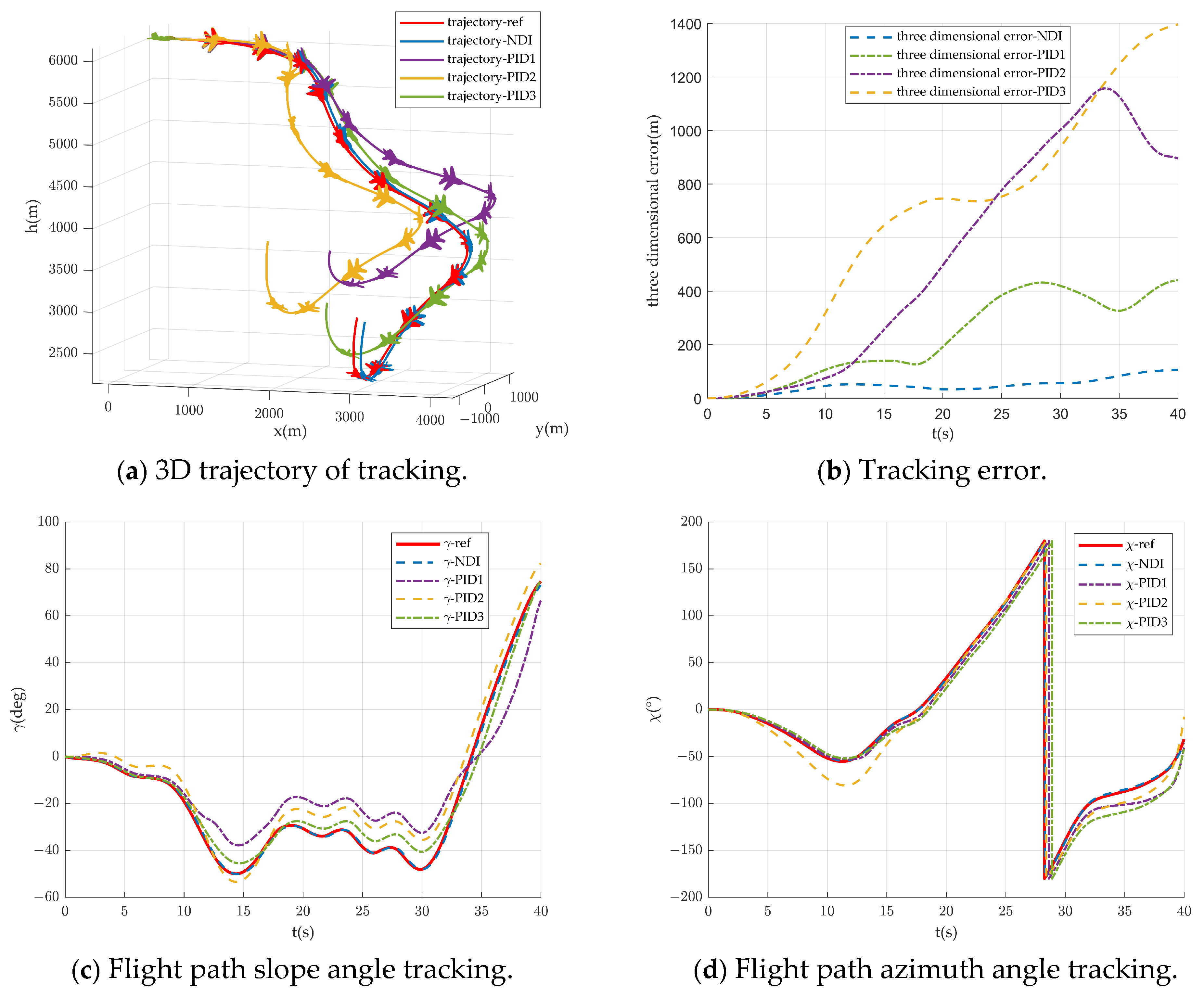
Figure 3 shows the simulation results of trajectory tracking control, and Figure 3a shows the 3D trajectory figure. The referenced trajectory in Figure 3a is a complex maneuvering trajectory, the vehicle firstly turns right and then turns left to hover and descend, and then climbs after finally changing to level; the whole maneuvering process has a large overload so that the effect of the trajectory tracking algorithm can be examined. From Figure 3a, it can be seen that the NDI algorithm can track the reference trajectory very well with very few errors. The flight trajectory of the PID1 algorithm can only be described as a shape approximation compared with the reference trajectory, and obviously the error is larger in both vertical and horizontal directions. The flight trajectory of the PID2 algorithm has a larger error in the vertical direction compared to the reference trajectory. The trajectory of the PID3 algorithm is more similar to the reference trajectory, but obviously the error is larger at the turn or climb.

Figure 3b shows the 3D trajectory error curve, where the NDI error is the smallest with a maximum error of 106 m, PID1 has a maximum error of 1394 m, PID2 has a maximum error of 1185 m, and PID3 has a maximum error of 441 m. The trajectory errors in Figure 3b are all in a continuous upward trend, which is due to the fact that the trajectory tracks the velocity, flight path slope angle, and flight path azimuth angle. The position changes in the kinematic equations are calculated from these three variables, so the tracking errors of velocity, flight path slope angle, and flight path azimuth angle lead to the accumulation of 3D trajectory position errors.

Figure 3c shows the tracking curve of the flight path slope angle, from which it can be seen that the NDI method can track the reference flight path slope angle curve well. The PID1 method has a certain overall error. The PID2 method obviously does not track the flight path slope angle, and the PID3 method tracks better most of the time, but there will be a certain error in the case of large overload.

Figure 3d shows the tracking curve of flight path azimuth angle, from which it can be seen that the NDI method can track the reference flight path azimuth angle curve well. The PID1 method tracks well in the middle part of the tracking curve, but the initial and final errors are larger. The PID2 method tracks with larger error in the last 10 s. The PID3 method shows some delay and error.

From the above analysis, it can be concluded that the NDI method significantly outperforms other tracking control methods in the literature in terms of tracking trajectory effectiveness, which is due to the accurate inverse solution for the angle of attack, roll angle, and thrust. PID2 has a significantly higher error due to the direct use of a referenced angle of attack. The overload calculation in PID1 is questionable, and, after modification, the tracking effect is better, but there is still some error at large overloads. The three-dimensional trajectory errors of the above methods all increase cumulatively with time.

4. Fast Trajectory Planning Based on Surrogate-Assisted Differential Evolutionary Algorithms (Decision Planning Layer)

In Section 3, due to the need to plan high-quality flight paths, it is clear that the use of a 3DOF model of overload and roll angle as a planning model is not feasible, since flight aerodynamic forces are not taken into account in the model and it could theoretically accelerate continuously. The use of the 3DOF model leads to an inaccurate representation of the aircraft energy concept. For example, energy maneuver theory suggests that an aircraft can only increase its energy state when its thrust is greater than its drag. The 3DOF model does not include any forces and therefore does not accurately capture this limitation. In the 3DOF model, the pilot can control the maximum speed with a positive flight path angle and climb forever, increasing its potential energy indefinitely—a major misunderstanding of aircraft dynamics.

To solve the problem, the flight dynamics equations in the trajectory coordinate system, assuming the side-slip angle and lateral force to be 0, are used for trajectory planning. The 5DOF model uses throttle, angle of attack, and roll angle as control variables to solve for lift and drag in real-time, thus planning trajectories with high fidelity.

It is generally accepted in the current literature that the real-time performance of maneuvering decisions using optimization algorithms is poor. Unlike the 3DOF model, the 5DOF model exacerbates the problem of real-time decision-making due to the need for real-time aerodynamic computation. The solution in this paper is to improve real-time decision planning by reducing the number of real fitness evaluations of the algorithms, using faster converging algorithms for maneuvering decisions, and using sampling and fitting to reduce the decision dimension.

In this section, in order to generate high-quality planning trajectories, a planning trajectory generator is first constructed using a 5DOF aircraft model, through which the maneuver decision problem is transformed into a decision variable optimization problem. And then the situation function is established as the objective function. In order to solve the problem of insufficient real-time performance of traditional intelligent optimization algorithms, a surrogate-assisted differential evolutionary algorithm is proposed on the basis of the original differential evolutionary algorithm and is compared with several other state-of-the-art algorithms in terms of the test function component as well as the maneuver decision problem.

4.1. Planning Trajectory Generator

Using Formula (7) in Section 3 as the dynamic model, combined with the kinematic model in the trajectory coordinate system, a 5DOF model can be obtained:

$$\left\{\begin{array}{l}\dot{x}=v\cos \gamma \cos \psi \hfill \\ \dot{y}=v\cos \gamma \sin \psi \hfill \\ \dot{z}=v\sin \gamma \hfill \\ \dot{v}={\displaystyle \frac{{\delta }_T{T}_{\max }\cos \alpha -D}{m}}-g\sin \gamma \hfill \\ \dot{\gamma }={\displaystyle \frac{(L+{\delta }_T{T}_{\max }\sin \alpha )\cos \mu }{mv}}-{\displaystyle \frac{g}{v}}\cos \gamma \hfill \\ \dot{\chi }={\displaystyle \frac{(L+{\delta }_T{T}_{\max }\sin \alpha )\sin \mu }{mv\cos \gamma }}\hfill \end{array}\right.$$

(23)

where $T_{\max }$ is the maximum engine thrust. The control variables $u={[\alpha ,\mu ,{\delta }_T]}^{\mathrm{T}}$ denotes angle of attack, roll angle, and throttle setting, respectively.

The dynamics model is the maneuver generator model, with which high-quality continuous aircraft trajectories can be generated. Since lift and drag calculations are used, the aircraft aerodynamic constraints are also taken into account so that the trajectories generated are of high quality and within the aerodynamic constraints of the aircraft.

In this paper, a 5DOF model is used for trajectory planning instead of a 6DOF model. The reason is that, in the process of generating the planned trajectory using the intelligent algorithm, several iterations of the kinematics and dynamics equations are required. The time consumption using the 6DOF model is much higher than using the 5DOF model.

Using angle of attack, throttle, and roll angle as control variables, and an iteration step of 0.02 s, a high-quality trajectory can be generated with a time length of 2 s. This trajectory requires 100 iteration cycles and, therefore, 100 control variable cycle inputs. In traditional maneuver action libraries or maneuver decision-making methods, the method of constant control variables in 1 s is often used, so the planning trajectory can be obtained quickly. However, this method is very different from the reality of continuous change in the control quantity, thus leading to the low quality of the decision trajectory and a large gap between the planning trajectory and the actual flight trajectory.

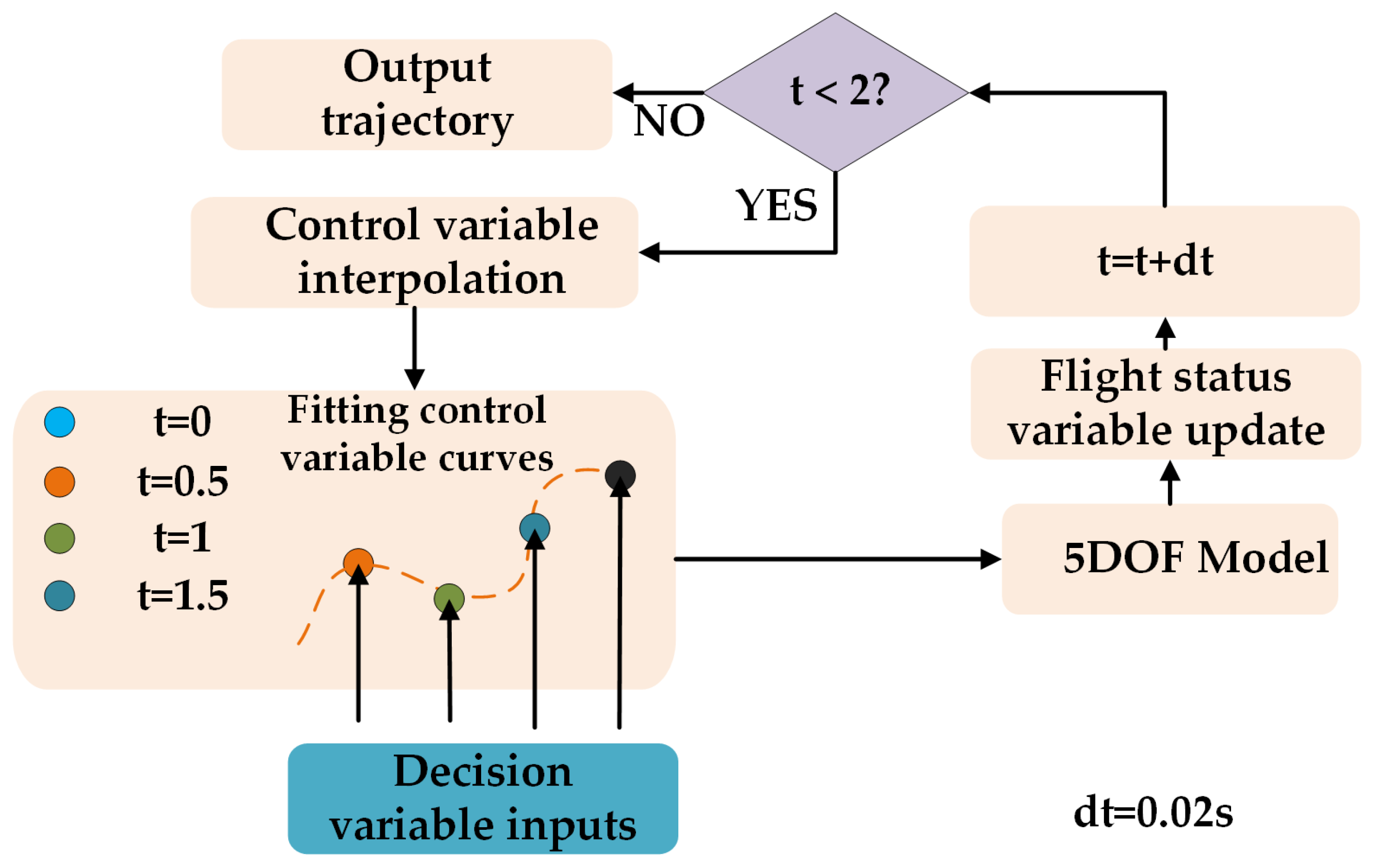
However, adopting each iteration cycle control variables as decision variables will lead to 100 × 3 decision dimensions, which will cause the optimization algorithm to be difficult to converge. To solve the problem, this paper adopts a compromise approach by adopting 0.5 s, 1 s, 1.5 s, and 2 s control variables as decision variables and using quadratic function fitting and interpolation to obtain the intermediate control variables. The flow chart is shown below.

The decision planning problem is transformed into a decision variable optimization problem by constructing a mapping from decision variables to trajectories through the method shown in Figure 4.

4.2. Objective Function Construction

In close air combat, the UCAV can only maintain the next moment situation advantage if only the next moment situation is considered. Without long-term consideration of the situation, the UCAV is easily deceived by adversary aircraft tactics. In this paper, the situation function after 2 s is taken as the objective function (where the adversary position is obtained using a trajectory prediction). The state information of the adversary aircraft after 2 s is obtained using a polynomial fitting prediction, and the method is not detailed here in view of the length of this paper.

4.2.1. Situation Assessment

In air combat geometry, angle and distance are usually considered to be the main factors constituting the air combat situation. Therefore, this paper establishes the angle situation function and the distance situation function and obtains the situation value by weighting.

4.2.2. Angular Situation Function

As shown in Figure 5, ${\lambda }_A$ is the bearing angle of UCAV and ${\lambda }_T$ is the aspect angle of adversary aircraft. The smaller ${\lambda }_A$ is, the more UCAV’s nose is pointing toward the adversary, and the smaller ${\lambda }_T$ is, the more UCAV is behind the adversary’s tail. Accordingly, the angular situation function is constructed as follows:

$$S_A={\displaystyle \frac{1}{2}}\left(1+\cos \left({\displaystyle \frac{1}{2}}({\lambda }_A+{\lambda }_T)\right)\right)$$

(24)

4.2.3. Distance Situation Function

The value of the distance situation function is only related to the distance between the enemy and the UCAV, not to the angle [12,15]. In fact, when the UCAV is in an angular advantage, the purpose of the UCAV is to close the distance in order to constitute a missile launching condition, whereas when the adversary aircraft is in an angular advantage, the purpose of UCAV is to move away from the adversary in order to avoid the adversary from constituting a missile launching condition. Accordingly, the distance situation function and the angular situation function are coupled to obtain the calculation method of the distance situation function, as shown below:

$$S_R=\left\{\begin{array}{c}0.5+(S_A-0.5)\max \left(0,{\displaystyle \frac{6R_0-d}{5R_0}}\right) \mathrm{if} d\ge R_0\\ 0.5+(S_A-0.5)\max \left(0,{\displaystyle \frac{d}{R_0}}\right) \mathrm{if} R_{\min }\le d<R_0\\ 0 \mathrm{else}\end{array}\right.$$

(25)

4.3. Surrogate-Assisted and Original Differential Evolutionary Algorithm

By analyzing the decision-making system constructed in this paper, in the updating of the discrete differential equation, it needs to be updated 100 times with a step size of 0.02 s to achieve the aircraft state after 2 s, and, in these 100 iterations, the values of the aircraft thrust and lift, as well as the drag force, need to be updated, which results in a large amount of computation and a long time-consumption time to speculate the flight state after 2 s. Therefore, the use of conventional trial maneuvering methods leads to a significant increase in decision time. For such optimization problems with few function evaluations, they can be regarded as expensive optimization problems, and the convergence efficiency of the intelligent optimization algorithm can be improved by establishing surrogate-assisted models.

4.3.1. Original Differential Evolution Algorithm

At the beginning of the optimization problem, DE stochastically generates populations in the search space. The individuals in the population create the next generation in an evolutionary manner. When the individual explores a new location with a better fitness value, the individual moves to that location. There are four main operators in DE, i.e., initialization, mutation, crossover, and selection operations [27]. Due to the limitation of space, the algorithm steps of the original DE algorithm will not be discussed in detail in this paper.

4.3.2. Surrogate-Assisted Differential Evolution Algorithm

Evolutionary algorithms are effective in overcoming the difficulties of multimodality, discontinuity, and non-differentiability that exist in many practical problems. Since the solution space of many problems is often uncertain or infinite, it is not feasible to rely on traversing the solution space to find a solution space. The evolution algorithm (EA) approximates the optimal solution gradually through exploration. However, most algorithms typically require multiple fitness function evaluations to obtain a feasible solution, which severely limits their ability to solve expensive engineering problems. For the maneuvering decision problem in this paper, the number of fitness function evaluations is limited due to real-time constraints, so surrogate-assisted differential evolutionary algorithms are used in this paper to solve this problem. Currently, surrogate-assisted evolutionary algorithms are flourishing and are widely used for expensive optimization problems and high-dimensional optimization problems. In most of these surrogate-assisted models, classification, regression, and interpolation techniques are used to approximate expensive objectives, such as Support Vector Machines (SVMs) [28], Gaussian Processes (GPs) [29], Radial Basis Functions (RBFs) [30,31], and Polynomial Regressions [32], among others.

The differences between the surrogate-assisted differential evolution algorithm proposed in this paper and the original differential evolution algorithm are as follows. (a) For the problem of the slow convergence of the original differential evolution algorithm, the “DE/current-to-best-w/r” strategy of the LSHADE-RSP [33] algorithm is introduced to improve the convergence efficiency of the algorithm. (b) For the selection operation of the original differential evolution algorithm, the selection operation is canceled because the offspring is evaluated by the surrogate model, not the real fitness evaluation, and, therefore, the selection operation constrains the evolution of the offspring. (c) The selection of the next real to-be-evaluated individual is crucial for the surrogate-assisted evolutionary algorithm, so the optimal offspring individual obtained from the surrogate model search is likely to fall into a local optimum. In this paper, the opposition-based learning strategy is used for the generation of real to-be-evaluated individuals, which gives the algorithm a certain chance of jumping out of the local optimum and improves the algorithm’s global exploration ability.

(a) Radial basis functions

The RBF model was originally developed for discrete multivariate data interpolation [34]. It uses a weighted sum of basis functions to approximate a complex landscape [35]. For a dataset consisting of input variable values and response values from N training points, the true function $\widehat{y}(x)$ can be approximated as follows:

$$\widehat{y}(x)=\sum _{i=1}^N{\lambda }_i\phi (\parallel x-c_i\parallel )+p(x)$$

(26)

where λ is the coefficient computed by solving the linear equation. C_i is the ith center of the basis function. P is either a polynomial model or a constant value; in this paper, linear polynomials are used [36]. $\phi$ is a basis function. Due to the uncertainty of (26), further orthogonality conditions are imposed on the coefficients:

$$\sum _{i=1}^N{\lambda }_i{p}_j(x_i)=0,\hspace{1em}\mathrm{for} j=1,2,\dots ,m$$

(27)

$$\left.\left(\begin{array}{cc}{\mathit{\Phi }}_{N,N}& {\mathit{P}}_{N,m}\\ {{\mathit{P}}_{N,m}}^T& \mathbf{0}\end{array}\right.\right)\left(\begin{array}{c}{\mathit{\alpha }}_{N,1}\\ {\mathit{c}}_{m,1}\end{array}\right)=\left(\begin{array}{c}{\mathit{F}}_{N,1}\\ \mathbf{0}\end{array}\right)$$

(28)

where m is the number of terms of $p(x)$ and Matrix $\mathit{\Phi }\in {\mathit{R}}^{N\times N}$ with element ${\mathit{\Phi }}_{ij}=\phi (\parallel x_i-x_j\parallel ),(i=1,2,\dots ,N),(j=1,2,\dots ,N)$. $\mathit{\alpha }={({\alpha }_1,{\alpha }_2,\dots ,{\alpha }_N)}^T\in R^N$ denotes a vector of weight coefficients. $P\in R^{N\times m}$ is a basis function matrix of linear polynomial $p(x)$ on the interpolating points, $\mathit{c}={(c_1,c_2,\dots ,c_m)}^T\in R^m$ is the vector of coefficients for the linear polynomial $p(x)$, and $F={(f(x_1),f(x_2),\dots ,f(x_N))}^T\in R^N$. Note that the coefficient matrix in Equation (28) is nonsingular as long as the interpolating points are all affinely independent [37].

(b) “DE/current-to-best-w/r” strategy

$$Ran{k}_i=k\cdot (N-i)+1$$

(29)

$$p{r}_i=Ran{k}_i/(Ran{k}_1+Ran{k}_2+\dots +Ran{k}_N)$$

(30)

$${\mathit{v}}_{i,g}={\mathit{x}}_{i,g}+F_i({\mathit{x}}_{best,g}^p-{\mathit{x}}_{i,g})+F_i({\mathit{x}}_{r1,g}-{\tilde{\mathit{x}}}_{r2,g})$$

(31)

where ${\mathit{x}}_{r1,g}$ denotes the individual selected from the current population P by the rank-based pressure selection strategy, and ${\tilde{\mathit{x}}}_{r2,g}$ is the individual selected from the current population P by the rank-based pressure selection strategy or randomly selected from the external archive A by the rank-based pressure selection strategy. The core idea of the rank-based pressure selection strategy is that the better the search individuals are, the higher the probability that they will be selected for the mutation strategy, thus increasing the convergence rate of the algorithm.

(c) Opposition-based search strategies

In general, the surrogate-assisted algorithm selects the optimal individual $P_{best}$ for RBF evaluation in pop(t + NP), but $P_{best}$ is easy to fall into the local optimum because of the multiple iterations of NG times. In this paper, the individual $P_{FE}$ generated by the opposition learning search strategy has a certain probability as the real evaluation individual, thus improving the ability of the algorithm to jump out of the local optimum.

Opposition-based learning search helps to improve the performance of the algorithm in exploring the global optimal solution. This strategy inversely maps the visited solutions in the search region to the unknown region. Reference [38] demonstrated that opposition-based learning search can help optimization algorithms to more closely match the global optimal candidate solutions. Equation (32) gives the manner in which the P_FE is generated when the algorithm performs an opposition-based search:

$$P_{FE}=(P_{best}+P_{max})\times r_2-P_{best}$$

(32)

where the poorest solution P_max and the current optimal solution P_best denote the upper bound and lower bound of the population. r₂ is a random number ranging from 0 to 1.

The pseudo-code of the Algorithm 1 is represented below.

Algorithm 1: SADE
Input: the number of initial sample points (K); the number of maximum FEs (maxNFE); predefined generation budget NG; swarm size (Np).
Output: The solution with the best fitness value: gbest and fbest
1:	Database initialization: Employ Latin Hypercube Design (LHD) to generate a uniformly distributed dataset, and archive it with exact fitness values into the database, NFEs = K
2:	While NFEs < maxNFE do
3:	Use all the samples to establish an RBF model
4:	Population initialization/re-initialization: Select Np top-ranking data from the database to form the initial population pop(g), set g = 0;
5:	RBF modeling/updating: Construct/update a global RBF model using all of the database samples;
6:	While g ≤ NG do
7:	Adopt “DE/current-to-best-w/r” and crossover to generate a new population pop(g + 1);
8:	Fitness estimation: Compute the fitness value of each individual in pop(t + 1) using the RBF model, set g = g + 1.
9:	End while
10:	Exact evaluation: Perform exact evaluation on the individual $P_{best}$ or $P_{FE}$, and archive it into the database; NFES = NFEs + 1
11:	End while

4.3.3. Algorithm Performance Validation

To examine the performance of SADE, SADE is implemented on a test suite consisting of five classical benchmark problems. SADE is compared with several state-of-the-art algorithms on selected benchmark problems. All compared algorithms were implemented in MATLAB R2016b and run on an Intel(R) Core(TM) i7-6500U CPU @ 2.50 GHz laptop, and each algorithm was executed for 30 independent runs for statistical analysis, respectively.

To evaluate the performance of the proposed algorithm, SADE is compared with algorithms such as GORS-SSLPSO [39], FSAPSO [40], LSHADE [41] and MPA [42]. Since the dimensionality of the decision variables of the motorized decision problem constructed in this paper is relatively small, it is tested only on a 10-dimensional benchmark problem. The GORS-SSLPSO and FSAPSO algorithms are advanced surrogate-assisted variations in particle swarm algorithms proposed in recent years. LSHADE is the winning algorithm of the CEC2014 competition, and MPA is an excellent population evolution-based intelligent algorithm proposed in 2021.

For a fair comparison, each competing algorithm is allocated a computational budget of 11 × D real fitness evaluations, and Figure 6 shows the results of SADE and the competing algorithms on the benchmark after 11D real fitness evaluations.

As can be seen from the iteration curves in Figure 6, the surrogate-assisted evolutionary algorithms have significantly better performance compared to other algorithms. SADE significantly outperforms the GORS-SSLPAO and FSAPSO algorithms on Ellipsoid, Rosenbrock, and Ackley, and is comparable to the GORS-SSLPSO and FSAPSO algorithms on Griewank and Rastrigin. The simulation results show that the introduction of the “DE/current-to-best-w/r” strategy of the SADE algorithm brings an improvement in the convergence efficiency, and, from the shape of the curves, the decrease in the SADE algorithm is more dramatic, which is related to the ability to break through the local optimum brought by the opposition-based search strategy.

4.3.4. Surrogate-Assisted Differential Evolutionary Algorithms for Autonomous Maneuvering Decisions

The SADE algorithm is used for the maneuver decision problem by using the situation function established above as the objective function. The UCAV and the adversary are in the same initial conditions, and one decision-making process is repeated 30 times as a comparison of the algorithms. The decision variables are used as inputs to the planning trajectory generator. The main time-consuming part of the algorithm is the planning trajectory generator, so the number of real fitness evaluation of the function is set to 50. comparing the SADE algorithm with the GORS-SSLPSO, FSAPSO, LSHADE, and MPA algorithms, the iterative curves can be obtained as shown below.

From Figure 7, it can be obtained that the situation value obtained using the SADE algorithm is superior to other comparative algorithms such as GORS-SSLPSO, FSAPSO, LSHADE and MPA. Under the condition of the same number of real fitness evaluations, SADE can obtain better situation values. The SADE algorithm average takes about 0.08 s for decision-making, the LSHADE algorithm and the MPA algorithm average take about 0.06 s because they do not use surrogate model, and the FSAPSO and GORS-SSLPAO algorithms take about the same time as the SADE algorithm. It is worth mentioning that the matrix game method average takes 0.2 s due to the use of the min-max search method [43], which is equivalent to the number of fitness evaluations of 7 × 7 × 7 times, and the obtained situation value is 0.49578, which is smaller than that of the SADE algorithm. The SADE algorithm is characterized by a short time-consumption time and strong optimization ability for the maneuvering decision problem.

4.4. Adaptive Tracking Error Correction and Planning Trajectory Splicing

It can be obtained through the controller comparison simulation that the tracking error will inevitably occur during the trajectory tracking process. As this paper tracks the values of the flight path slope angle and flight path azimuth angle and speed, so, similar to the next layer of the differential equation, the three-dimensional coordinate error will increase with time and the error will slowly accumulate, so it is necessary to correct the tracking error. As shown in Figure 8, the three-dimensional coordinate error is corrected at the planning starting point. When the three-dimensional coordinate error is larger than the threshold value, the actual three-dimensional coordinates are used as the planning starting point, and when the flight path slope angle and flight path azimuth angle errors are larger than the threshold value, the flight path slope angle and flight path azimuth angle are corrected. Meanwhile, for the former planning trajectory and the latter planning trajectory, when the error does not exceed the threshold value, the method of splicing the planning trajectory is adopted, which also makes the controller more stable and does not have the situation where the error suddenly goes to zero.

5. Simulation Experiments

In this section, in order to verify the superiority of the algorithm proposed in this paper, the simulation verification of the adversary aircraft and UCAV confrontation takes the method of confrontation with the same flight model. Both the adversary aircraft and UCAV adopt the 6DOF model of F-16 airplane, which is divided into four initial scenarios, namely head-on neutral, dominant, parallel neutral, and disadvantaged, according to the different initial situation of the adversary and us. The red side is the UCAV with the SADE algorithm, and the blue side is the adversary UCAV with the LSHADE algorithm, the original DE algorithm, the min–max search algorithm, and the random search algorithm, respectively.

The initial situation of the setup is shown in

Table 1. Initial scene setting.

Scenario	UCAV	x/m	y/m	z/m	V/[m/s]	χ/deg
Case 1	red	0	0	6000	220	0
	blue	10,000	10,000	6000	220	180
Case 2	red	0	0	6000	220	0
	blue	4000	1000	6000	220	0
Case3	red	0	0	6000	220	0
	blue	0	1000	6000	220	0
Case4	red	0	0	6000	220	0
	blue	−2500	2000	7000	220	0

.

The number of real fitness evaluations of the algorithm is set to 50, the number of populations is set to 60, the unit maneuver time is 2 s, and the simulation step size is 0.02 s. According to the geometry of the air combat, the termination condition of the simulation is defined as 400 < R < 2000, and the bearing angle of the UCAV is less than 15 degrees, while the aspect angle of the adversary aircraft is less than 105 degrees. Under this condition, the UCAV is in a tailing situation, and missiles can be launched to hit the adversary aircraft, and it is therefore judged to win the air combat.

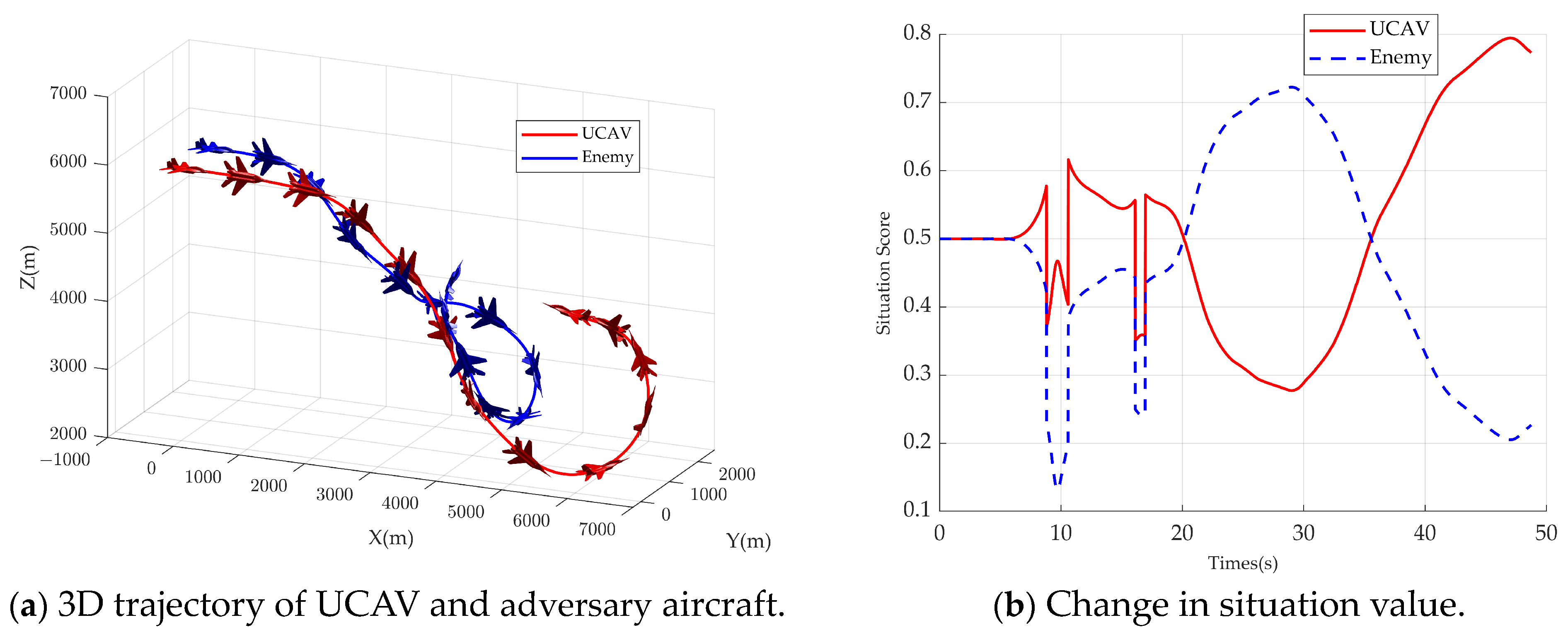
5.1. Initial Head-On Neutral Situation

In the initial head-on neutral posture, the initial flight path azimuth angles of the UCAV and the adversary are 0 and 180 degrees, respectively, with the same initial altitude and speed. The UCAV adopts the SADE algorithm and the adversary airplane adopts the LSHADE algorithm. The simulation results are shown in Figure 9. The UCAV’s trajectory figure is shown in Figure 9a, from which it can be seen that both the adversary aircraft and the UCAV take similar maneuvers, which is due to the same situation function, and it can be seen that the adversary and the UCAV’s trajectories form the classic single loop in the BFM, which demonstrates decision-making ability close to the tactical level of humans. In the initial phase, the adversary and the UCAV approached head-on. At about 33 s, when the adversary and the UCAV intersected, the adversary had a slight advantage in the angular posture due to the larger overload of the UCAV, and then the UCAV reduced its turning radius by decreasing its normal overload and keeping its speed lower than the adversary’s, which successfully made the adversary aircraft rush forward. At about 74.26 s, the UCAV and the adversary aircraft formed a trailing situation, reaching the termination conditions of the simulation, and the UCAV won the air combat.

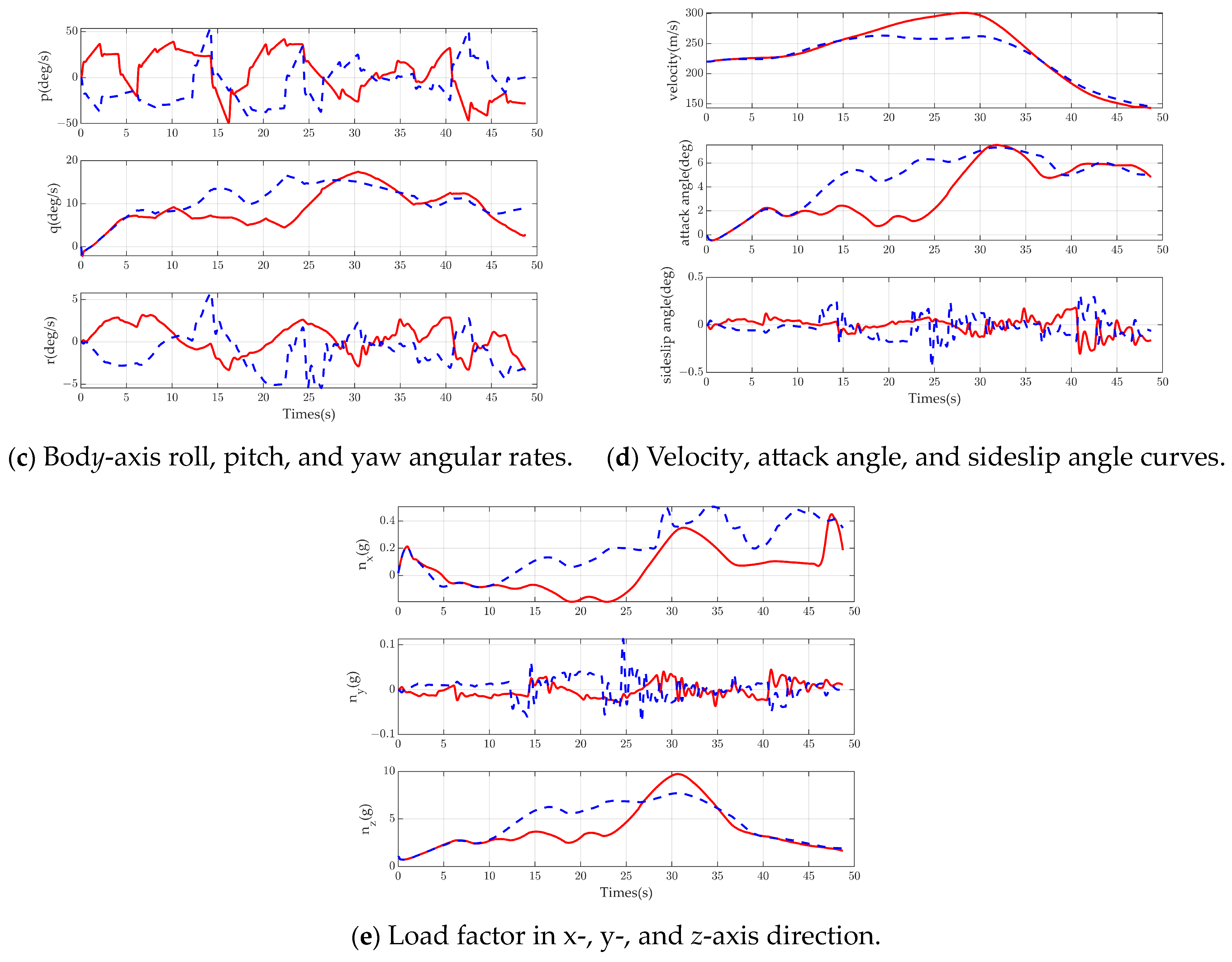
As can be seen in Figure 9b, there are two steep drops in the adversary and UCAV situation function values due to the small distance when the adversary and the UCAV crossed paths. The adversary aircraft gained some situational advantage around 33 s, and then the UCAV gained a situational advantage until the end of the simulation. The roll, pitch, and yaw rate curves under the bod y-axis system are shown in Figure 9c, in which q stably stays around 10 deg/s and p changes more drastically, indicating that the roll changes are intense. The speed of the UCAV in Figure 9d is less than that of the adversary aircraft, which reduces the turning radius and obtains the situational advantage. The sideslip angle beta is kept within 0.2 degrees, proving the effectiveness of nonlinear dynamic inverse control. In Figure 9e, the normal overload can reach more than 5 g, proving the intensity of the air combat confrontation of the maneuver decision method.

5.2. Initial Dominant Situation

In the initial dominant situation, the UCAV is initially behind the tail of the adversary aircraft, and the initial flight path azimuth angle is the same. The UCAV adopts the SADE algorithm, and the adversary aircraft adopts the original DE algorithm. The simulation results are shown in Figure 10, where (a) is the 3D trajectory diagram, and it can be seen that the adversary aircraft adopts a right-turn circling maneuver in order to get rid of the UCAV, and, at this time, the UCAV adopts a straight-line maneuver to close the distance, so the adversary aircraft’s situation increases. Figure 10b shows that the adversary’s situation reached about 0.45, but then the UCAV also took a right-turn downward circling maneuver; at this time, the UCAV regained the situation advantage, and, finally, the UCAV formed a tailing situation to achieve the termination conditions of the simulation and achieved victory in the air combat.

The roll, pitch, and yaw rate curves under the body axis system are shown in Figure 10c, and it can be seen that the p change in the UCAV is more intense, while the p change in the adversary aircraft is more gentle, which indicates that the UCAV has a drastic change in roll while the adversary aircraft is continuously performing a right-handed circling with a small change in roll.

In Figure 10d, the initial speed of the UCAV is the same as that of the adversary aircraft, but the speed of the UCAV increases significantly due to the large drop in altitude. In addition, the UCAV initially flies flat, so the angle of attack is small, and then the angle of attack increases after the turn. The UCAV side-slip angle is maintained at a size of less than 0.2 degrees.

In Figure 10e, since the speed of the UCAV increases significantly when it is circling downward, it is obvious that the normal overload is larger than that of the adversary aircraft at a similar angle of attack to the adversary aircraft, which reaches about 10 g. This phenomenon is that the aerodynamic lift receives double the effect of speed and angle of attack, so the overload increases when the speed increases.

5.3. Initial Parallel Neutral Situation

Under the initial parallel neutral situation, the adversary aircraft and the UCAV are relatively close to each other and are in the same flight direction. The UCAV adopts the SADE algorithm and the adversary aircraft adopts the min–max search algorithm. The simulation results are shown in Figure 11, where Figure 11a is the 3D trajectory figure, from which it can be seen that the adversary aircraft and the UCAV initially take a similar maneuver, producing two crossovers. It is reflected in Figure 11b that there are two steep decreases in the situation value, which is due to the close distance, so the value of the distance situation suddenly changes to 0. Then the UCAV and the adversary aircraft did a descending circle to the right and to the left, respectively; because the UCAV descended faster and with a larger speed, it had a larger turning radius and fell into a situation of disadvantage. Then the adversary did a right turn and climb maneuver, and the UCAV did a combat turn maneuver, thus turning the situation into an advantage. From the trajectory, it can be seen that both the adversary and the UCAV performed complex maneuvers, which reflects the strong decision-making ability of both the adversary and the UCAV.

Figure 11c shows the angular rate variation curves. The values of body axis roll and yaw rate fluctuate around zero. The adversary and UCAV velocity changes in Figure 11d are similar, with the UCAV having a larger velocity due to a larger drop in altitude in the middle section. The initial angle of attack is larger for the adversary aircraft, so the initial overload is higher for the adversary aircraft, as shown in Figure 11e.

5.4. Initial Disadvantaged Situation

Under the initial disadvantaged situation condition, the initial UCAV is in the situation of being trailed by the adversary aircraft, the UCAV is in the same heading as the adversary aircraft, and the UCAV is in the right front of the adversary aircraft. The UCAV adopts the SADE algorithm, and the adversary aircraft adopts the random search method. The simulation results obtained are shown in Figure 12, where Figure 12a is the 3D trajectory figure. As can be seen from Figure 12a, firstly, the UCAV adopts left turn circling descent to get rid of the situation disadvantage, and the adversary aircraft adopts right turn firstly in order to close the distance, and then it also adopts left turn circling descent maneuver, but then the UCAV quickly adopts right turn maneuver so as to form a single loop with the adversary aircraft. In the end, the UCAV, due to its smaller speed and smaller turning radius, gained the situation advantage, formed a tail chase, reached the termination conditions of the simulation, and won the air battle.

As can be seen in Figure 12b, the UCAV situation values are steadily increasing. In Figure 12c, the body axis system roll rate changes dramatically. In Figure 12d, the initial speed of the UCAV is the same as that of the adversary aircraft, but after that, the UCAV speed is less than that of the adversary aircraft, so it has a smaller turning radius and gains a situation advantage. In the first half of the confrontation, the angle of attack of the UCAV is relatively large, which is because the initial UCAV situation is at a disadvantage, and the rapid increase in overload can get rid of the disadvantage. In Figure 12e, the maximum overload during the confrontation can reach 8 g, reflecting the intensity of the confrontation.

5.5. Simulation Statistics

In order to fairly evaluate the performance of the algorithms, 100 simulations of each algorithm were conducted in each initial situation, and the results were categorized as win, fail, and neutral. The results are judged as win when the UCAV reaches the termination condition or the adversary aircraft crashes, fail when the adversary aircraft reaches the termination condition or the UCAV crashes, and neutral when the simulation max time is reached with no loss on either side.

In the four initial situations of head-on neutral, dominant, parallel neutral, and disadvantaged situations, the blue aircraft used LSHADE, original DE, min–max search, and random search algorithms, respectively, and the red aircraft used the different algorithms from the blue aircraft. The win ratio in the figure is calculated from the perspective of the red side. The results are shown in Figure 13.

In Figure 13, the SADE algorithm achieves more than a 53% win rate in all four initial situation conditions. Due to the randomness of intelligent optimization algorithms, the SADE algorithm cannot achieve victory in every game, but it can significantly improve the win rate. The LSHADE algorithm and the original DE algorithm also show a competitive performance, and the min–max search algorithm performs similarly to the LSHADE algorithm, but it takes longer. The random search algorithm is inferior to other algorithms due to the randomness of the search, and it has a low win rate under initial dominance conditions.

6. Conclusions

In this paper, a hierarchical maneuver decision and control framework based on a surrogate-assisted differential evolutionary algorithm is proposed which divides the air combat maneuver decision process into a decision planning layer and a tracking control layer. In the decision planning layer, the maneuver decision problem is transformed into an optimization problem, and SADE is used to obtain a high-quality planning trajectory under the condition of a limited number of real fitness evaluations. In the tracking control layer, a nonlinear dynamic inverse tracking control method is used to track the planning trajectory and realize the high-precision control of a 6DOF vehicle. Simulation results show that in the tracking control layer, compared to the traditional PID algorithm, the nonlinear dynamic inverse control algorithm tracks the planning trajectory with less error and higher accuracy. In the decision planning layer, the SADE algorithm has strong search capability and decision accuracy and can effectively drive the UCAV to obtain the air combat victory in head-on neutral, dominant, parallel neutral, and disadvantaged situations, which can effectively improve the air combat victory rate compared to the traditional min–max search algorithm and random search algorithm.

This paper’s method is applicable to airplanes with different aerodynamic coefficients, while existing deep reinforcement learning methods need to be retrained for each different airplane, which is an advantage of this paper’s method. The main disadvantages of this paper’s method are that the algorithm’s decision-making capability is limited by the situation function.

In future work, missiles will be added to participate in the confrontation. The method of this paper can be considered as an adversary of reinforcement learning methods for training purposes. Eventually, the algorithms of this paper will be applied to real outfield aircraft and experiments will be conducted.