Figure 1.
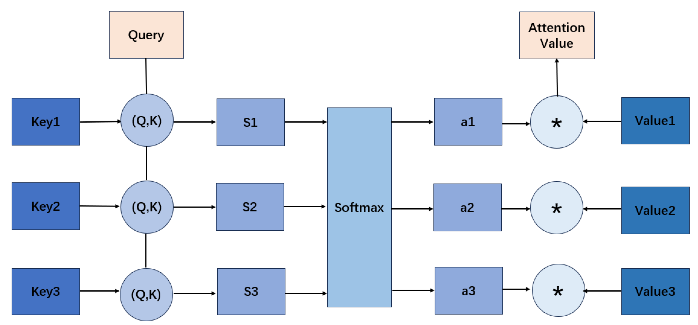
Schematic of scaled dot-product attention: relevance is computed via , normalized by softmax, and applied to V to form the context.
Figure 1.
Schematic of scaled dot-product attention: relevance is computed via , normalized by softmax, and applied to V to form the context.
Figure 2.
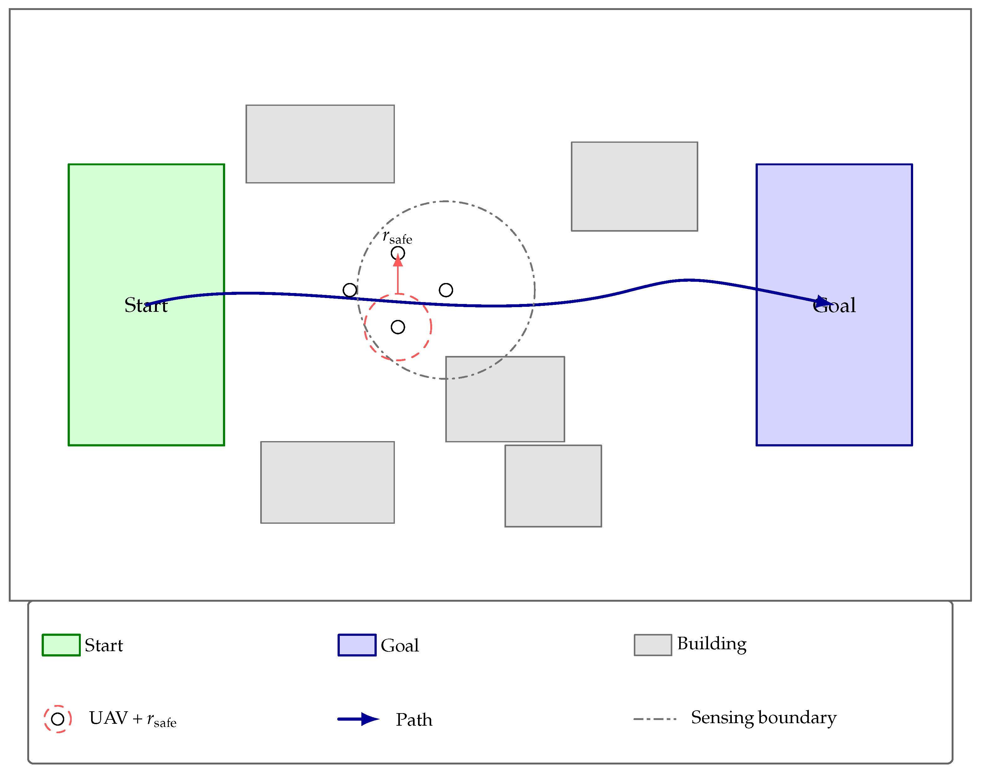
Problem setup (top view). Workspace: m, m, m. Buildings are within ; half-length/width m, height m (cap 20). Initial region: ; target region: . Example radii for illustration: sensing radius m, safety radius m. The legend is placed below the map to avoid any overlap with the environment elements.
Figure 3.
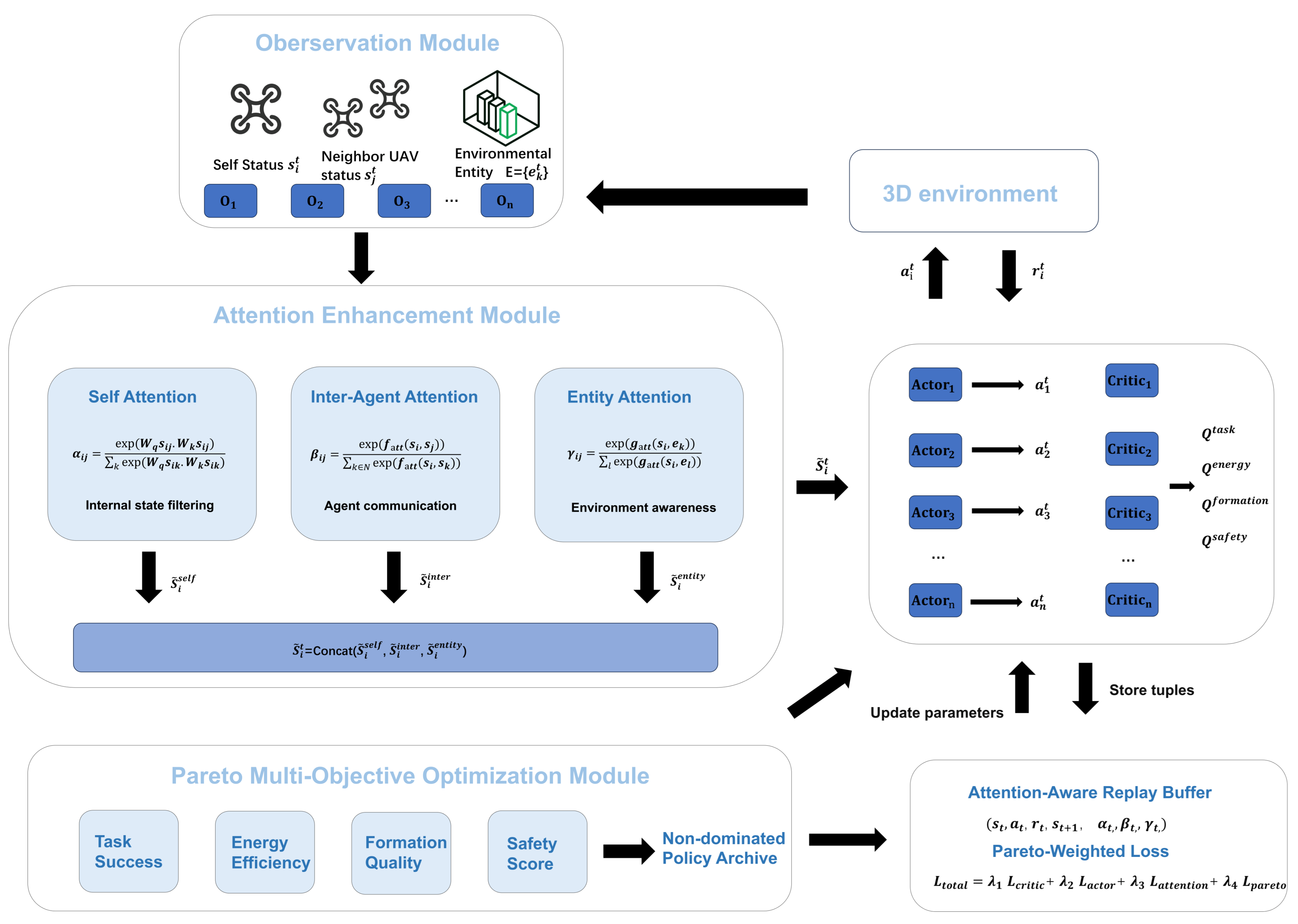
Overall framework: plug-and-play attention (self/inter-agent/entity) before each decentralized actor, and a Pareto layer over vector critics during centralized training. We instantiate with a MADDPG backbone for concreteness, but the modules are applicable to other CTDE actor–critic MARL algorithms.
Figure 4.
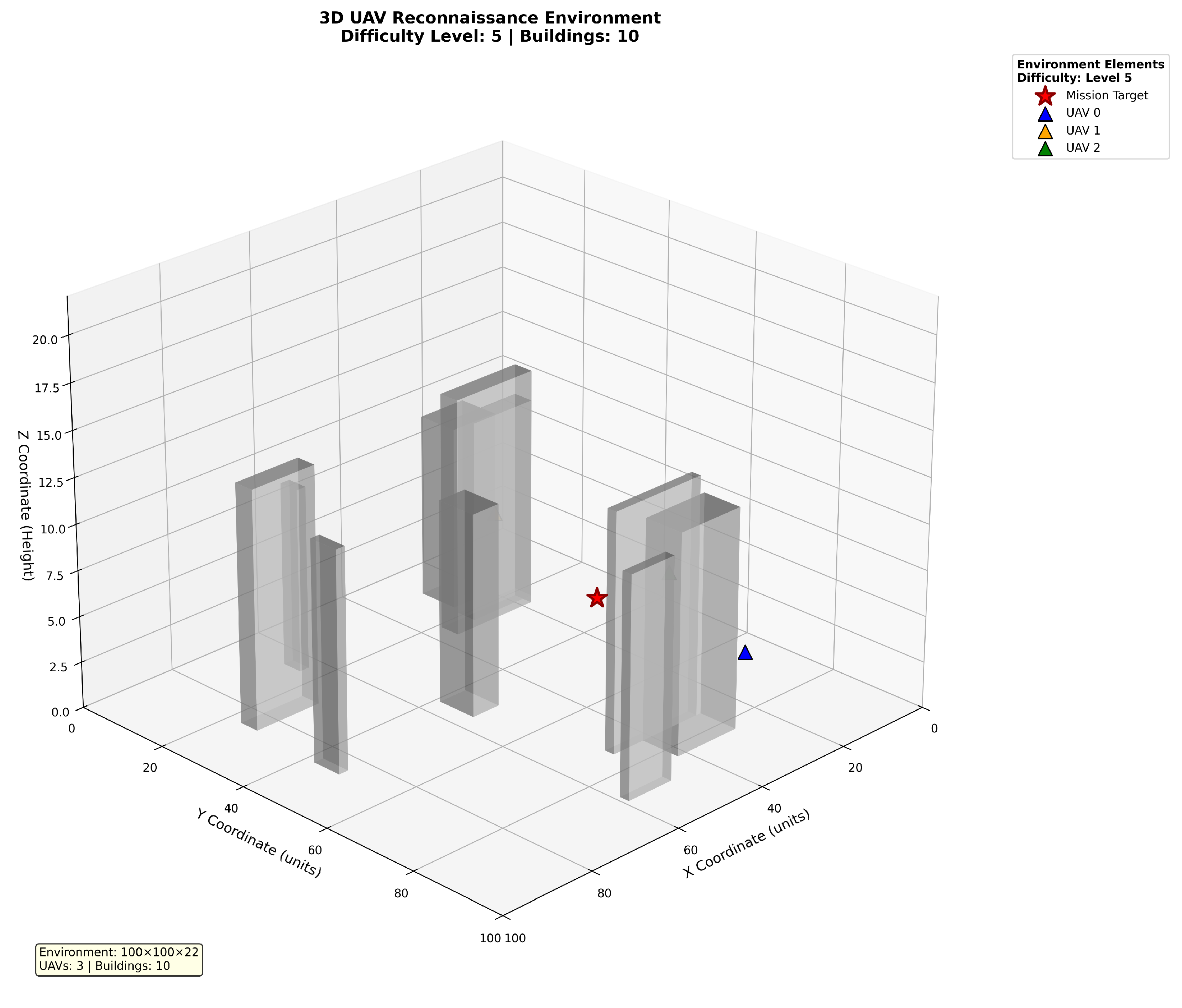
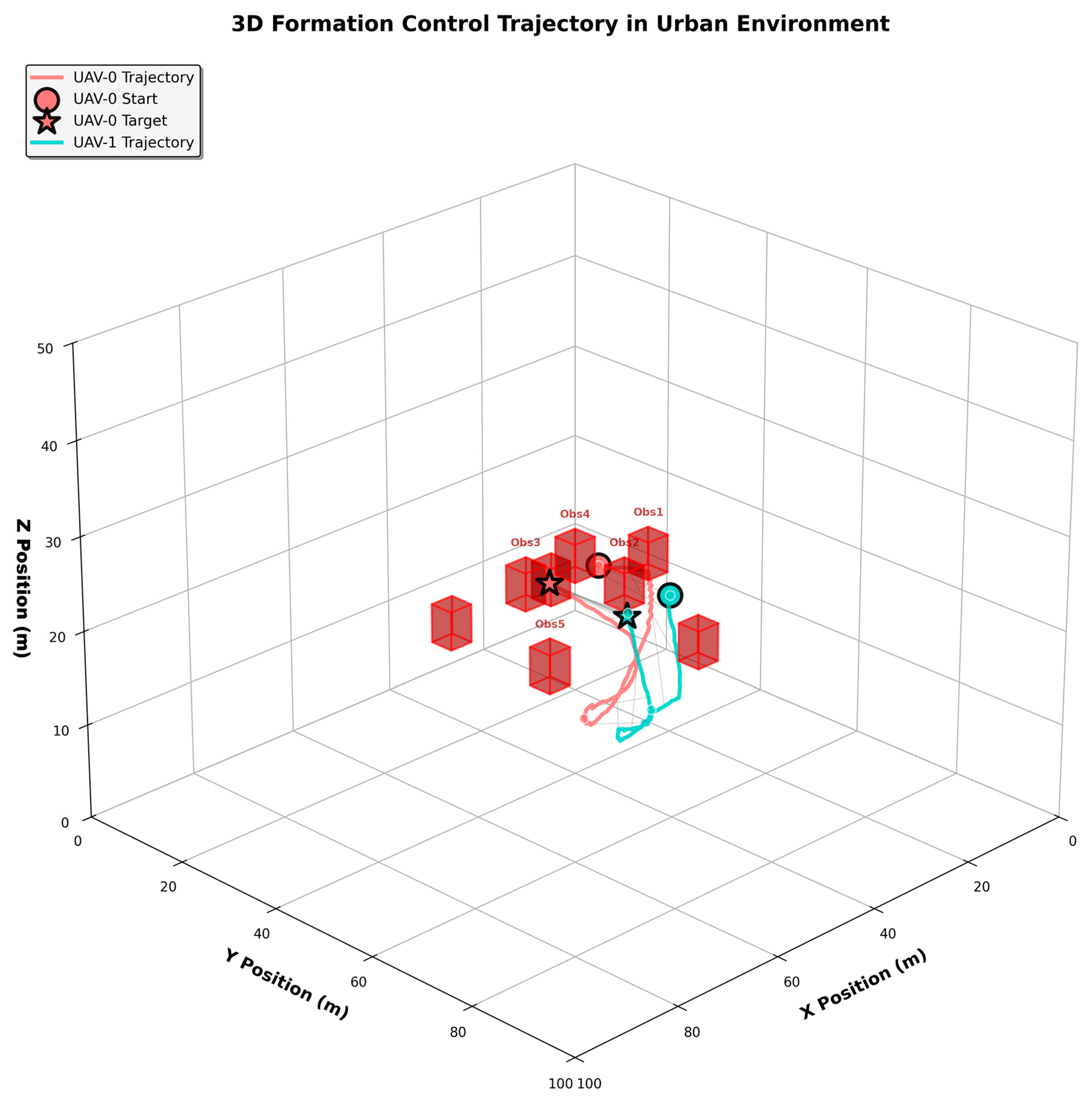
Three-dimensional environmental schematic diagram.
Figure 4.
Three-dimensional environmental schematic diagram.
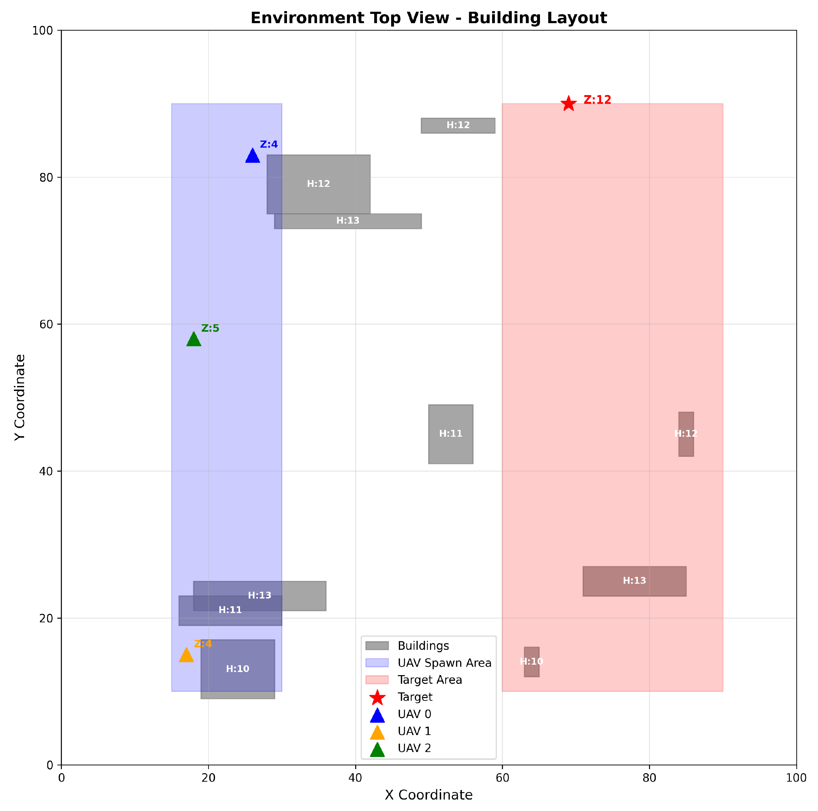
Figure 5.
Two-dimensional top view of the environment.
Figure 5.
Two-dimensional top view of the environment.
Figure 6.
This combo graph shows the training curves of success rate for 2-agent in 10,000 episodes.
Figure 6.
This combo graph shows the training curves of success rate for 2-agent in 10,000 episodes.
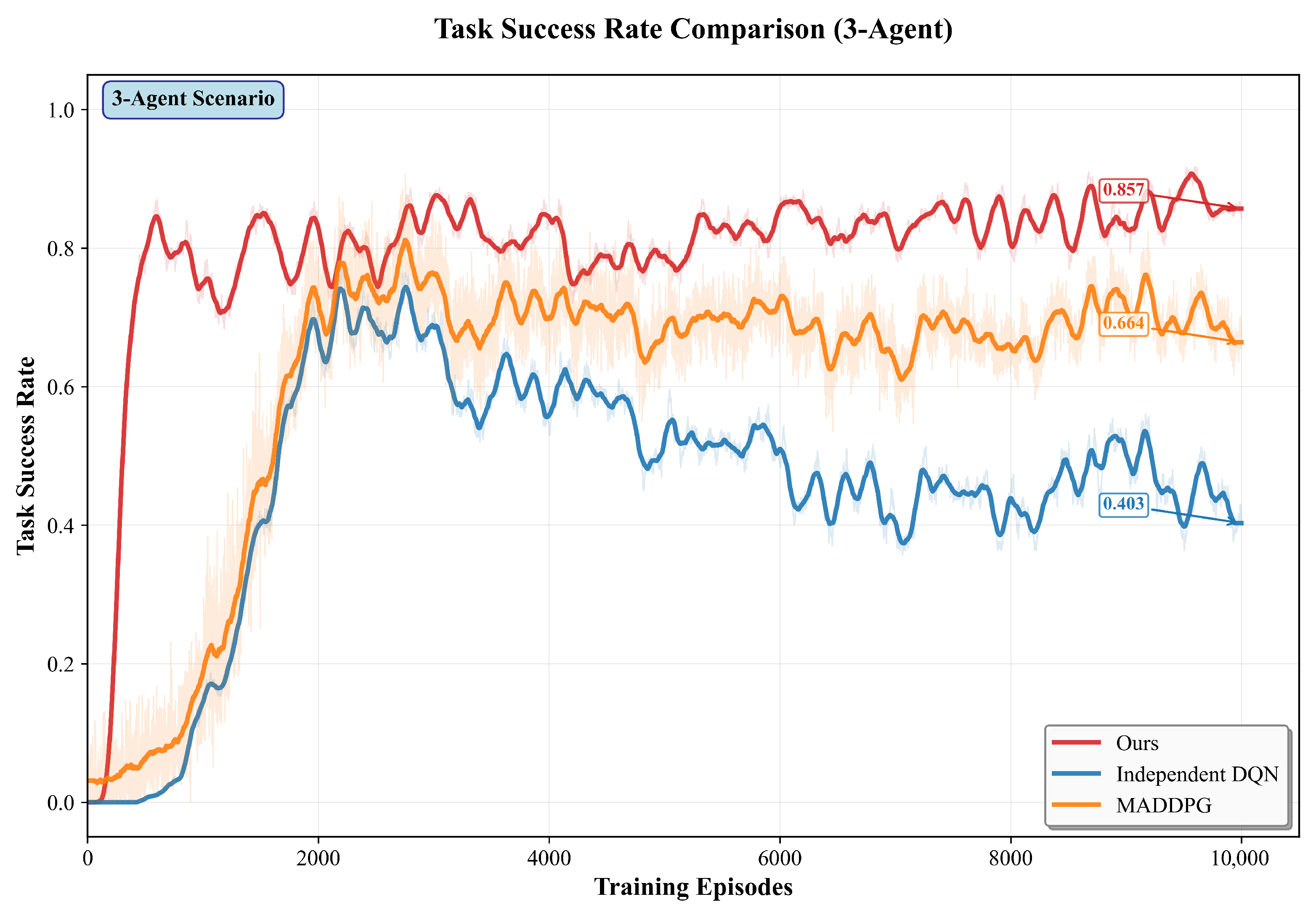
Figure 7.
This combo graph shows the training curves of success rate for 3-agent in 10,000 episodes.
Figure 7.
This combo graph shows the training curves of success rate for 3-agent in 10,000 episodes.
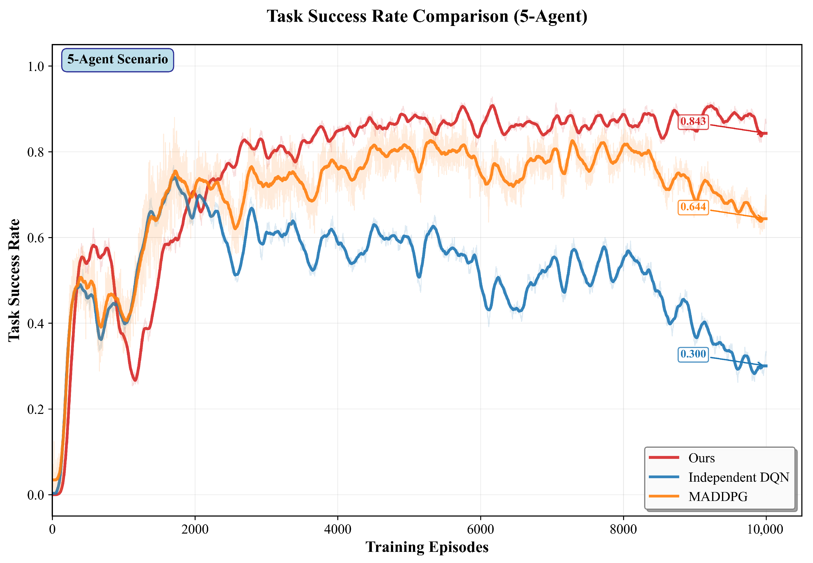
Figure 8.
This combo graph shows the training curves of success rate for 5-agent in 10,000 episodes.
Figure 8.
This combo graph shows the training curves of success rate for 5-agent in 10,000 episodes.
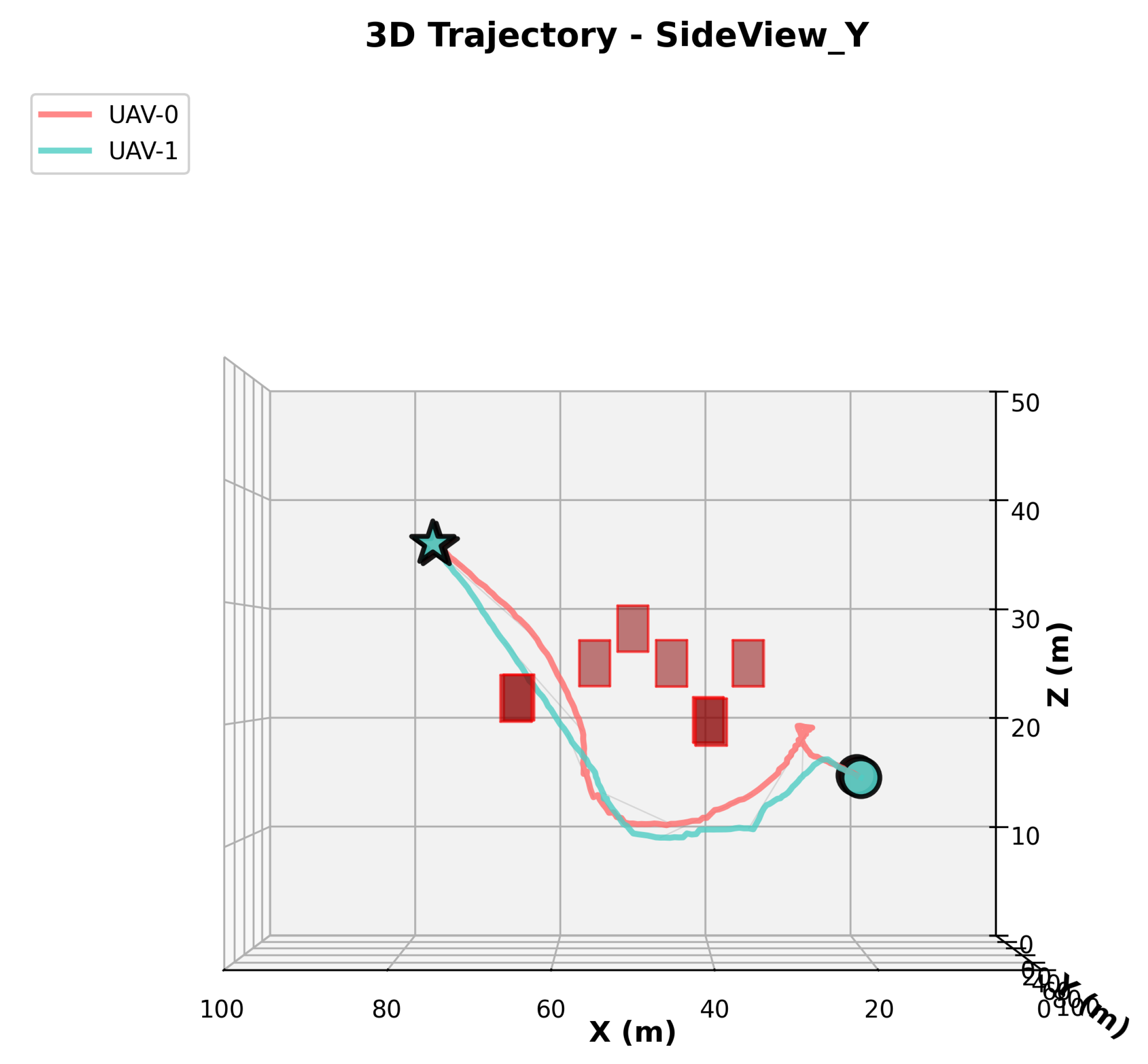
Figure 9.
Representative top-down trajectories comparing ours, MADDPG, and IDQN (best seed per method; same map). Ours shows earlier widening and fewer sharp re-plans near bottlenecks.
Figure 9.
Representative top-down trajectories comparing ours, MADDPG, and IDQN (best seed per method; same map). Ours shows earlier widening and fewer sharp re-plans near bottlenecks.
Figure 10.
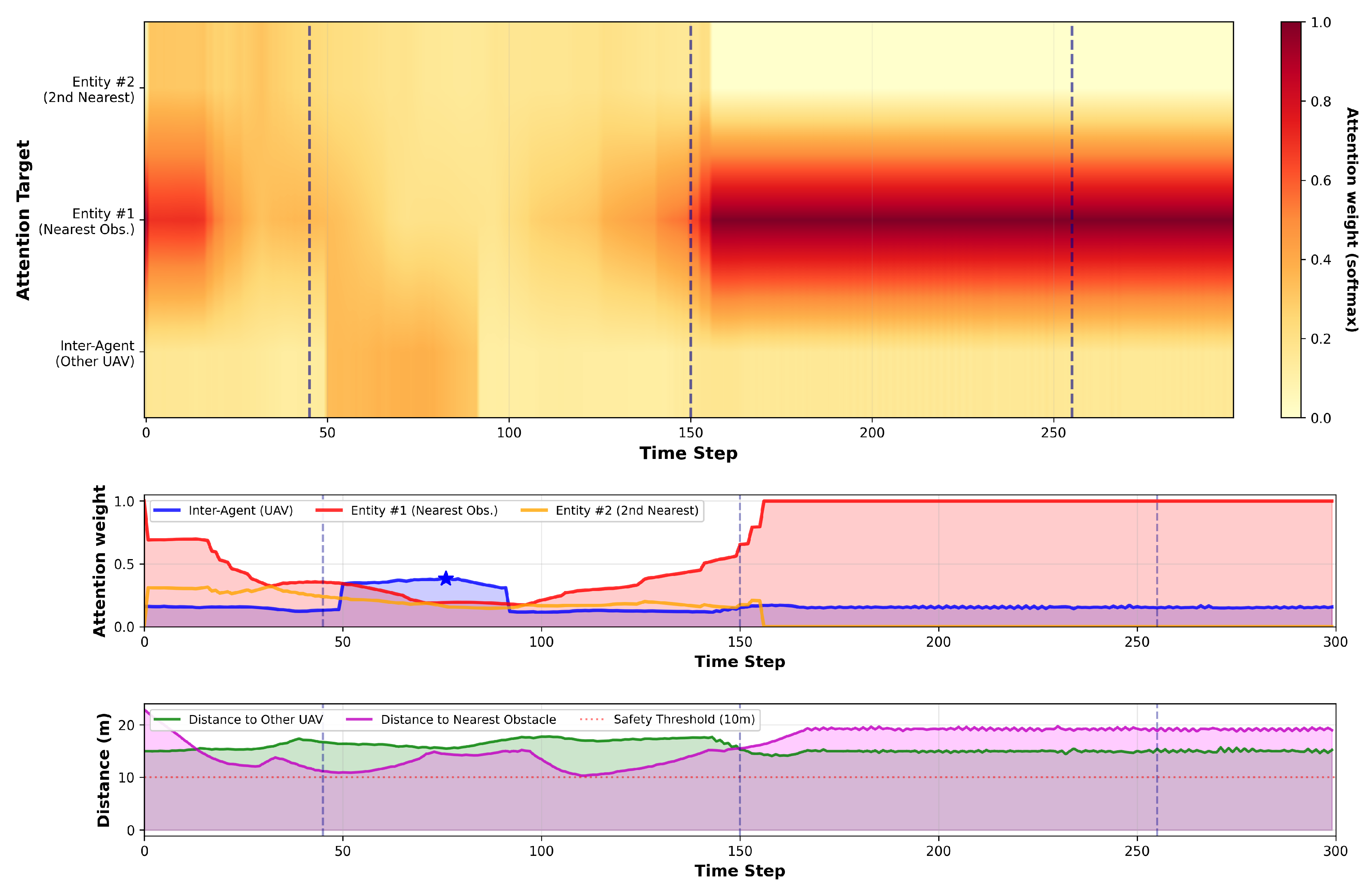
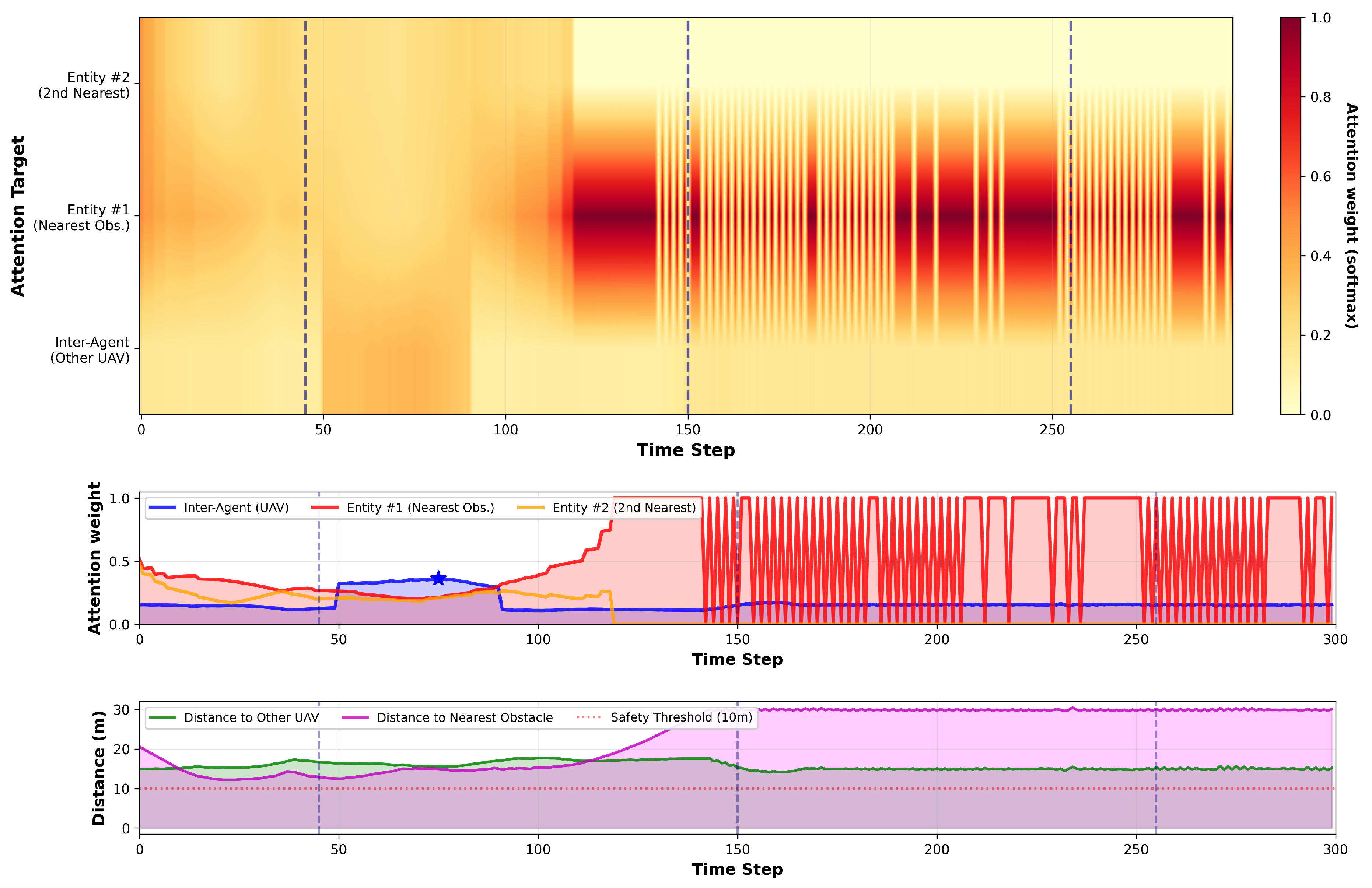
Attention dynamics during a representative flight (seeded, no exploration). Each panel shows, from top to bottom: (i) a heatmap over time of inter-agent vs. entity attention (softmax; colorbar in [0, 1]); (ii) attention-weight time series for the inter-agent branch and the two nearest obstacles; (iii) spatial distances (inter-UAV, nearest obstacle) with the safety threshold for context. Vertical dashed lines mark the timestamps visualized in
Figure 11.
Figure 11.
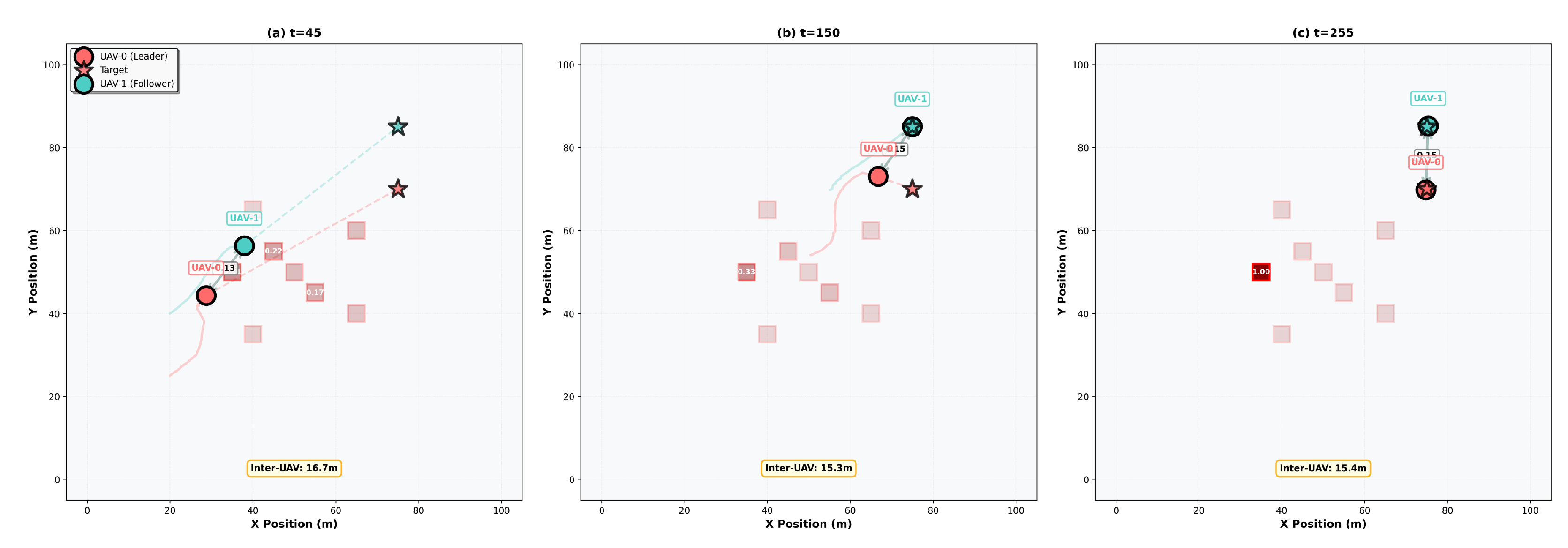
Top-down snapshots at three timestamps (left to right:
,
,
) from the same rollout as
Figure 10. Edge thickness encodes inter-agent attention from the focal UAV, while obstacle shading (and labels) encodes entity attention.
Figure 11.
Top-down snapshots at three timestamps (left to right:
,
,
) from the same rollout as
Figure 10. Edge thickness encodes inter-agent attention from the focal UAV, while obstacle shading (and labels) encodes entity attention.
Table 1.
Architectural contrast between PA-MADDPG and stacked GNN/Transformer front ends.
Table 1.
Architectural contrast between PA-MADDPG and stacked GNN/Transformer front ends.
| Aspect | PA-MADDPG (This Work) | GNN-Based MARL (Stacked) | Transformer-Based RL (Stacked) |
|---|
| Mixing scope | Single-hop KNN neighbors + M entities; typed branches; concat | L-layer message passing; L-hop receptive field | Self/cross-attn over all tokens; global mixing per layer |
| Complexity per step | with fixed fan-in | , | , |
| Latency/memory | Low; on-board friendly | Medium–high; grows with | High; quadratic in tokens |
| Heterogeneity handling | Typed (self/inter/entity); no type embeddings | Requires typed edges/engineering | Needs token-type/ positional encodings |
| Communication model | Masked KNN; renormalized attention | Fixed/learned graph; often reliable links | Often assumes global broadcast |
| Training signal | Vector critics + Pareto (multi-objective) | Usually scalarized reward | Usually scalarized reward |
| Primary goal | Real-time local control | Expressive multi-hop reasoning | Global context/long-range mixing |
Table 2.
Hyperparameters of the proposed multi-agent attention-DRL framework.
Table 2.
Hyperparameters of the proposed multi-agent attention-DRL framework.
| Category | Parameter | Value |
|---|
| Network Architecture | Actor hidden layers | [256, 128] |
| | Critic hidden layers | [512, 256, 128] |
| | Attention dimension | 64 |
| Training | Actor learning rate | |
| | Critic learning rate | |
| | Batch size | 256 |
| | Replay buffer size | |
| | Discount factor | 0.99 |
| | Soft-update | 0.01 |
| Attention | Self-attention heads | 4 |
| | Inter-agent range (m) | 10.0 |
| | Entity attention range (m) | 15.0 |
| Pareto Archive | Archive size | 100 |
| | Update frequency | 10 steps |
Table 3.
Notation used in the formulation.
Table 3.
Notation used in the formulation.
| Symbol | Description |
|---|
| Agent set and its size |
| Time index, horizon, and time step |
| Global state, local observation, and action |
| G | Goal pose/region encoding |
| Formation template and per–agent slot offset |
| Set of M nearest buildings (centers and half–sizes) |
| K | Number of neighbor slots in |
| Reward vector in (7) |
| Discount factor |
| Decentralized policy and joint policy |
| Per objective centralized critic in (13) |
| Action bound, safety distance, goal threshold |
Table 4.
N = 2, five-seed statistics for average team success rate (%). Mean ± s.d. and two-sided CIs (Student-t, ).
Table 4.
N = 2, five-seed statistics for average team success rate (%). Mean ± s.d. and two-sided CIs (Student-t, ).
| Method | Mean ± s.d. (%) | 95% CI (%) |
|---|
| Ours | | |
| MADDPG | | |
| IDQN | | |
Table 5.
N = 2, pairwise comparisons on average team success (%). Welch’s t-test (two-sided), with degrees of freedom (df), p-value, and Hedges’ g. is the mean difference in percentage points (pp).
Table 5.
N = 2, pairwise comparisons on average team success (%). Welch’s t-test (two-sided), with degrees of freedom (df), p-value, and Hedges’ g. is the mean difference in percentage points (pp).
| Comparison | (pp) | t (df) | p-Value | Hedges’ g |
|---|
| Ours vs. MADDPG | | | | |
| Ours vs. IDQN | | | | |
Table 6.
Team success rate (%) after training.
Table 6.
Team success rate (%) after training.
| Method | | | |
|---|
| PA-MADDPG (ours) | 84.6 | 83.1 | 81.7 |
| MADDPG | 57.4 | 70.4 | 68.6 |
| IDQN | 47.8 | 58.1 | 55.7 |
Table 7.
Ablation study results of attention modules. Bold entries indicate the best (most favorable) result among all configurations for each metric.
Table 7.
Ablation study results of attention modules. Bold entries indicate the best (most favorable) result among all configurations for each metric.
| Configuration | Success Rate (%) | Formation Dev. (m) | Collision Rate (%) | Energy Efficiency |
|---|
| Full Model | 88.7 ± 1.8 | 1.47 ± 0.15 | 3.2 ± 0.8 | 0.86 ± 0.04 |
| w/o Entity Attention | 87.1 ± 2.3 | 1.89 ± 0.21 | 4.7 ± 1.1 | 0.81 ± 0.05 |
| w/o Inter-Agent Attention | 82.4 ± 2.8 | 2.15 ± 0.26 | 6.3 ± 1.4 | 0.78 ± 0.06 |
| w/o Self-Attention | 85.7 ± 2.5 | 1.98 ± 0.23 | 5.1 ± 1.2 | 0.79 ± 0.05 |
| w/o All Attention | 78.5 ± 2.8 | 2.31 ± 0.22 | 6.8 ± 1.2 | 0.74 ± 0.06 |
Table 8.
Baseline weighted-sum reward configurations. Notes: Safety-focused increases the penalty/weight for collisions and near-misses while keeping task progress moderate; Task-focused increases goal-reaching progress terms and success bonuses; Energy-focused increases control-effort regularization and discourages actuation bursts; Formation-focused tightens slot-tracking terms and rewards small formation RMSE; Balanced applies uniform scalarization across all objectives. All variants share the same architecture and training schedule and differ only in reward scalarization.
| Configuration | | | | |
|---|
| Safety-Focused | 0.4 | 0.1 | 0.2 | 0.3 |
| Task-Focused | 0.5 | 0.2 | 0.2 | 0.1 |
| Energy-Focused | 0.3 | 0.4 | 0.2 | 0.1 |
| Formation-Focused | 0.3 | 0.1 | 0.5 | 0.1 |
| Balanced | 0.25 | 0.25 | 0.25 | 0.25 |
Table 9.
Quantitative comparison of Pareto and weighted-sum methods.
Table 9.
Quantitative comparison of Pareto and weighted-sum methods.
| Method | Task Success | Formation Quality | Energy Efficiency | Safety Score | Overall Score |
|---|
| Safety-Focused | 84.2 ± 2.1 | 0.78 ± 0.05 | 0.71 ± 0.06 | 0.94 ± 0.02 | 0.82 |
| Task-Focused | 91.1 ± 1.9 | 0.75 ± 0.06 | 0.69 ± 0.07 | 0.83 ± 0.04 | 0.80 |
| Energy-Focused | 82.7 ± 2.3 | 0.72 ± 0.07 | 0.89 ± 0.03 | 0.81 ± 0.05 | 0.81 |
| Formation-Focused | 85.4 ± 2.0 | 0.92 ± 0.03 | 0.68 ± 0.08 | 0.79 ± 0.06 | 0.81 |
| Balanced | 87.3 ± 2.2 | 0.83 ± 0.04 | 0.76 ± 0.05 | 0.85 ± 0.03 | 0.83 |
| Pareto (Ours) | 88.7 ± 1.8 | 0.91 ± 0.04 | 0.86 ± 0.04 | 0.93 ± 0.02 | 0.91 |
Table 10.
Robustness evaluation under different perturbations (absolute degradation from nominal 88.7%).
Table 10.
Robustness evaluation under different perturbations (absolute degradation from nominal 88.7%).
| Condition | Success Rate (%) | Performance Degradation (pp) |
|---|
| Nominal | 88.7 ± 1.8 | – |
| Sensor Noise () | 85.4 ± 2.1 | 3.3 |
| Sensor Noise () | 82.3 ± 2.8 | 6.4 |
| Learning Rate +20% | 87.9 ± 2.3 | 0.8 |
| Learning Rate | 86.5 ± 2.0 | 2.2 |
| Attention Dim ±25% | 85.7 ± 2.2 | 3.0 |
| Archive Size ±30% | 87.2 ± 1.9 | 1.5 |
Table 11.
Per-UAV normalized energy proxy (mean ± s.d.; lower is better).
Table 11.
Per-UAV normalized energy proxy (mean ± s.d.; lower is better).
| Team Size | Ours | MADDPG [16] | IDQN [17] |
|---|
| 0.86 ± 0.04 | 0.93 ± 0.05 | 0.97 ± 0.06 |
| 0.84 ± 0.05 | 0.91 ± 0.05 | 0.95 ± 0.06 |
| 0.83 ± 0.05 | 0.90 ± 0.05 | 0.94 ± 0.06 |
Table 12.
Zero-shot robustness under networking impairments (single run; 100-episode moving average at end of evaluation). Note: results are from a single run; “±” denotes the standard deviation over the last 100 episodes (moving window).
Table 12.
Zero-shot robustness under networking impairments (single run; 100-episode moving average at end of evaluation). Note: results are from a single run; “±” denotes the standard deviation over the last 100 episodes (moving window).
| Setting | Success Rate (%) |
|---|
| Nominal (no loss, no delay, static topo) | 88.7 ± 1.8 |
| 79.2 ± 1.5 |
| ms | 71.2 ± 2.4 |
| link/s (time-varying topology) | 81.6 ± 2.2 |
Table 13.
Runtime profile (mean over 3 runs; RTX 4090/i7-12700). Team-step latency refers to one environment step for the whole team.
Table 13.
Runtime profile (mean over 3 runs; RTX 4090/i7-12700). Team-step latency refers to one environment step for the whole team.
| N | Method | Team-Step (ms, GPU) | FPS (GPU) | GPU RAM (GB) | Team-Step (ms, CPU) | FPS (CPU) |
|---|
| 2 | Ours | 0.55 | 1810 | 0.9 | 3.2 | 312 |
| 2 | MADDPG | 0.50 | 2000 | 0.8 | 2.9 | 345 |
| 3 | Ours | 0.72 | 1390 | 1.1 | 4.1 | 244 |
| 3 | MADDPG | 0.66 | 1510 | 1.0 | 3.7 | 270 |
| 5 | Ours | 1.05 | 950 | 1.4 | 6.8 | 147 |
| 5 | MADDPG | 0.97 | 1030 | 1.3 | 6.1 | 164 |
Table 14.
Training throughput (environment steps per second, mean ± s.d., RTX 4090).
Table 14.
Training throughput (environment steps per second, mean ± s.d., RTX 4090).
| N | Ours | MADDPG | IDQN |
|---|
| 2 | | | |
| 3 | | | |
| 5 | | | |

