Highlights
What are the main findings?
- Tractable mathematical derivations of UAV height-dependent spectrum occupancy reveal the impact of different types of 3D antenna patterns.
- Ray tracing-based analysis with a real-world 3D map and realistic antenna setup verifies the analytical trend of height-dependent spectrum occupancy.
What is the implication of the main finding?
- As UAV height increases, spectrum occupancy decreases and converges to a constant value.
- The spectrum occupancy trend with respect to 3D antenna patterns and UAV height should be carefully considered when optimizing 3D cellular networks.
Abstract
Unmanned aerial vehicles (UAVs) are emerging as mobile aerial platforms for radio frequency (RF) spectrum sensing, enabling dynamic monitoring of the spectrum occupancy of cellular systems at different altitudes. The impact of UAV receiver antenna configurations, particularly with respect to altitude, is critical in determining occupancy performance. In this paper, we present a height-dependent analytical framework for UAV-based spectrum occupancy, focusing on how different receiver antenna configurations affect the sensed signal power. We consider two types of 3D antenna patterns: a typical dipole antenna and a downward directional antenna. Using a stochastic geometry-based approach, we derive closed-form expressions for the altitude-dependent sensed power under both antenna configurations. Moreover, we execute ray tracing-based analysis with a real-world 3-D map and realistic antenna patterns. Monte Carlo simulations are conducted to validate the analytical results, revealing that both altitude and antenna directivity critically affect occupancy accuracy and coverage.
1. Introduction
With the advantage of flexibility of deployment and operation, unmanned aerial vehicles (UAVs) have been widely utilized in various applications, including surveillance, smart farming, and aerial transportation and delivery. Furthermore, UAVs play a key role in advanced wireless communications. For instance, UAV-mounted base stations (BSs) have been investigated to provide real-time connectivity for ground users in outage regions [1,2]. In addition, UAVs can be operated as aerial spectrum sensors to monitor spectrum occupancy, assisting in efficient radio emission mapping without the need for dense fixed ground sensor networks [3,4].
As the demand for reliable UAV connectivity grows across urban, suburban, and rural environments, cellular-connected UAVs have become a key enabler of seamless communication and large-scale operations beyond visual line-of-sight (BVLOS). Recently, advanced air mobility (AAM) and urban air mobility (UAM) have emerged as promising unmanned transportation services by facilitating autonomous mobility [5,6]. In such scenarios, maintaining robust communication and awareness of spectrum usage conditions is critical—particularly at varying altitudes. UAVs equipped with directional beamforming antennas can also serve as aerial integrated sensing and communication (ISAC) platforms, simultaneously performing communication and spectrum sensing functions to observe aggregate uplink activity and detect spectrum occupancy levels in real time [7,8]. This enables altitude-aware monitoring of RF environments, which supports both communication reliability and spectrum coexistence strategies. Furthermore, the altitude-dependent line-of-sight (LoS) probability between ground transmitters and UAV receivers plays a crucial role in determining network performance [9,10]. Therefore, it is essential to investigate how UAV altitude and antenna configuration affect the spectrum occupancy performance to optimize network design for future aerial communication systems.
Owing to their analytically tractable nature, stochastic geometry models have been extensively applied in the literature to evaluate the performance of cellular wireless networks, where multiple signal sources are spatially distributed according to a specified node density. Although several studies have analyzed the impact of UAV altitude on the aggregate received signal power from spatially distributed ground-based signal sources, many studies have assumed that aggregate interference remains independent of UAV altitude [11,12,13]. However, such assumptions do not align with recent spectrum occupancy measurements collected via UAV-based receivers [14,15,16], which show that the sensed spectrum availability varies significantly with altitude due to changes in propagation conditions. In particular, the aggregate received signal power gradually converges to a constant level as the UAV altitude increases.
In refs. [17,18], the air–ground channel model has been investigated through experiments under LoS conditions. Ref. [17] shows that the path loss can be well characterized by a two-ray model, implying the free space path loss exponent. In ref. [18], a path loss exponent of 2.03 was measured for the link between an access point (AP) and a quadcopter. The LoS probability function has been studied in refs. [19,20]. In ref. [19], an LoS probability model for urban street environments was introduced, characterized by street width and building height. In ref. [20], the LoS probability was modeled using a sigmoid (S-curve) function based on parameters recommended by the International Telecommunication Union (ITU) [21]. In this context, in this work, we adopt the free space path loss exponent for the LoS conditions, and use an approximated LoS probability function derived from the ITU-recommended model [21].
In this paper, we investigate how different types and beamwidth configurations of UAV receiver antennas impact cellular spectrum occupancy as a function of UAV height. We consider two types of receiver antennas: the typical dipole antenna and the downward directional antenna. In our prior work, we analyzed altitude-dependent cellular spectrum occupancy using a stochastic geometry-based framework that incorporated ray-tracing simulations and empirical measurements [16]. However, that study did not account for the effects of the receiver antenna pattern of the UAV spectrum sensor, despite its significant impact on occupancy behavior. A comparative summary of the related works is listed in Table 1. The analytical findings and simulation results in this study provide valuable insights into the spectrum occupancy characteristics under different UAV receiver antenna configurations in the optimization of UAV-based wireless communication networks.

Table 1.
Summary of existing related works.
Contributions of this paper can be summarized as follows:
- –
- In our prior works [14,16], we analyzed UAV altitude-dependent spectrum occupancy based on measurement campaigns, stochastic-geometry analysis, and ray-tracing simulations under the omnidirectional antenna assumption. As an extension of these studies, we investigate the impact of different types of 3D antenna patterns on altitude-dependent spectrum occupancy.
- –
- By incorporating rectangular antenna models to represent dipole and downward-directional antennas, we derive closed-form expressions for the aggregate received signal power and demonstrate its decreasing and converging behavior with increasing UAV altitude.
- –
- The stochastic-geometry-based results show that the downward-directional antenna configuration achieves a higher average aggregate received power than the dipole antenna in urban environments, whereas the dipole antenna performs better in suburban environments. In addition, a wider beamwidth configuration yields a higher average aggregate received power in urban scenarios.
- –
- Ray-tracing simulation results with realistic antenna designs show that a narrow beamwidth leads to higher average aggregate received power for the downward-directional antenna, while a wider beamwidth provides higher power for the dipole antenna.
2. System Model
We consider a scenario involving UAV interference from terrestrial cellular network signal sources. In uplink frequency bands, the signal sources are user equipment (UE) on the ground, whereas in downlink frequency bands, the signal sources are eNBs/gNBs. The power of aggregate signals received at the UAV from terrestrial signal sources in a given spectrum band characterizes the UAV’s cellular spectrum occupancy in that frequency band. The UAV’s cellular spectrum occupancy varies with height due to changes in the channel conditions of individual links from signal sources. In this paper, we focus on spectrum occupancy in uplink cellular bands.
We utilize a stochastic-geometry-based approach to analyze cellular spectrum occupancy as shown in Figure 1. We assume that the spatial distribution of UE follows a homogeneous Poisson point process (HPPP) on an infinite 2D plane with a constant node density . A typical UAV is deployed at the origin at a height of . The UAV is equipped with an antenna designed with a 3D directional radiation pattern. The horizontal and 3D distances between UE and the UAV are denoted as and , respectively. In addition, the channel condition between a UE and the UAV can be either LoS or NLoS, depending on the presence of obstacles along the direct path.
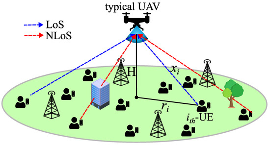
Figure 1.
Illustration of the UAV’s cellular spectrum occupancy scenario.
3. Cellular Spectrum Occupancy Model
In this section, we derive the expression for the aggregate received signal power at a typical UAV, introduce a mathematically tractable model for LoS probability, and present a 3D antenna pattern model in a mathematically tractable form.
3.1. Average Aggregate Received Signal Power
The aggregate received signal power at a typical UAV from ground UE allocated within the spectrum of interest can be expressed as follows:
where , f, c, , , , and represent the small-scale fading component, the carrier frequency, the speed of light, the transmit power and transmitter antenna gain of UE, the receiver antenna gain of the typical UAV, and the pathloss exponent, respectively. Note that we assume a flat-fading channel model followed by Rayleigh or Nakagami, where frequency selectivity is neglected due to the sufficiently narrow bandwidth. Then, the expectation of aggregate received signal power is given by
where receiver antenna gain is a function of given the UAV height due to the 3D directional antenna pattern. Note that the receiver antenna patterns are modeled in Section 3.3. In the second line of (2), we assume that the small-scale fading is normalized such that the expectation of the small-scale fading is for both LoS and NLoS conditions. Considering the LoS probability, and by applying Campbell Theorem [22], the expectation of aggregate received signal can be rewritten as
where and denote the pathloss exponent of LoS and NLoS conditions, respectively, and the approximation of (3) comes from a uniform UE density with respect to instead of , and indicates the LoS probability depending on the given the UAV height . To simplify the closed-form derivation, we assume the reasonable value of pathloss exponent of LoS and NLoS as and , which correspond to free-space propagation and additional blockage losses, respectively. Then,
3.2. Line-of-Sight Probability Function
The probability of geometrical LoS between a terrestrial transmitter and a receiver at height of can be modeled in a single expression as [20]
where , and , , and are three statistical parameters representing the type of the environment, which represent the ratio of built-up land area, the mean number of buildings per unit area, and the height distribution of buildings, respectively. For tractable closed-form analysis, alternatively, we adopt the closely approximated version of the LoS probability expression in (5) using a break-point exponential function formula as [16]
where represents the break-point distance where the probability function transitions from a constant value to an exponential decay, and and are environmental fitting parameters where the values are fitted to and for urban and suburban environments, respectively. These values correspond to the environmental parameters , , and in (5). Note that although the approximated expression in (6) exhibits an abrupt decrease at the breakpoint, the slope of the decrease beyond the breakpoint closely matches that of the exact expression in (5) (Figure 2, [16]), resulting in negligible errors in the average aggregate received signal power.
3.3. Three-Dimensional Antenna Pattern Modeling
The receiver antenna on the UAV follows an angle-dependent 3D antenna pattern, which is omni-directional in the azimuth domain but directional in the elevation domain. This type of receiver antenna pattern can be either a vertically oriented typical dipole antenna or a directional antenna implemented with a uniform planar array (UPA). In this section, we formulate these antenna patterns into mathematically tractable expressions.
3.3.1. Rectangular Antenna Pattern Model
We consider a rectangular beam model for the elevation angle-dependent directional antenna patterns. Note that although the rectangular antenna pattern model cannot fully represent the realistic antenna patterns, this model still effectively captures the key effects of antenna directivity and beamwidth depending on the antenna type, while maintaining analytical tractability. The rectangular beam pattern is given by
where [degree], [degree], and G [dBi] denote the lowest angle of the beam, the half-power beamwidth, and the maximum antenna gain, respectively. Next, by modifying the expression in (7) as a function of 3D distance x given , we can obtain
3.3.2. Antenna Directivity
In general, a narrower beamwidth in an antenna pattern results in a higher maximum antenna gain due to the concentration of radiated power in a specific direction. In this model, the antenna gain is normalized to ensure that the total radiated power remains constant. The total radiated power by an antenna is given by
where denotes azimuth angle. By considering the omni-directional pattern in the azimuth plane and using the rectangular antenna pattern model in (7), we can rewrite (9) as
By using the condition that the total radiated power by the antenna is equal to the constant value, the maximum antenna gain is given by (Chapter 2.2.6, [23])
where is the beam solid angle.
3.3.3. Types of Antennas
As described above, we consider two types of antennas: the typical dipole antenna and the downward directional antenna. Figure 2 illustrates the shape of the 3D antenna pattern of these two antennas. When we apply the rectangular antenna pattern model in Section 3.3.1, the typical dipole antenna holds , while the downward directional antenna holds . By applying these properties to (11), the maximum antenna gain in (8) for each antenna type can be expressed by
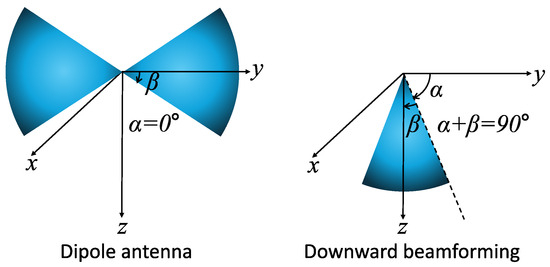
Figure 2.
Three-dimensional antenna patterns of two types of 3D antenna model.
4. Closed-Form Expression and Height-Dependent Analysis
In this section, we derive the closed-form expression of the average aggregate received signal power, as given in (4), by using the LoS probability function and the 3D antenna models in Section 3. Moreover, we analyze the height-dependent behavior of cellular spectrum occupancy based on the derived expressions.
4.1. Closed-Form Expression of Typical Dipole Antenna
In this subsection, we derive the closed-form expression for the average aggregate signal power for a typical dipole receiver antenna. Based on the relative magnitude of the half-power beamwidth and the environmental parameter of in the LoS probability function, the closed-form derivation depends on two cases, Case D-1 and Case D-2. In (8), by applying the property of the typical dipole antenna (), the range of the x covered by the beam becomes , while the integral range of three terms in (13) is determined by . Therefore, the closed-form expressions vary with the relative magnitude of and .
4.1.1. Case D-1
By applying the condition of Case D-1 and (12), (13) can be reformulated as
where denotes the upper incomplete gamma function, and we apply the property of . Note that the second term in (14) is a positive value since this term represents the aggregate power of the NLoS component. This implies that the multiplicative term in parentheses in front of remains positive. Thus, the average aggregate power in (14) decreases as increases.
4.1.2. Case D-2
Similar to the analysis of Case D-1, the third term in (15) is a positive value since this term represents the aggregate power of the NLoS component. Thus, the average aggregate power in (15) monotonically decreases as increases.
Figure 3a illustrates three distinct regions determined by the LoS/NLoS conditions and the directional antenna patterns in Case D-2, which is implied in the derived expression in (15). The first term in (15) corresponds to the full LoS region, where the integral range of x is from to . The second and third terms, which have the same integral range of x from to infinity, represent the contributions from LoS and NLoS conditions in the LoS + NLoS region. The absence of an integral term for x from 0 to indicates the outage region. As described in Figure 3a, as the UAV height increases, the outage and full LoS regions expand, while the LoS+NLoS region shrinks. In (15), the first and the second terms are constant values, which means that the average aggregate signal power of UE in the LoS condition is not affected by the UAV height. On the other hand, the third term decreases with increasing UAV height, implying that the average aggregate signal power decreases due to the contribution of NLoS UE in the LoS+NLoS region.
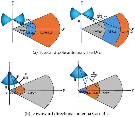
Figure 3.
The outage, LoS, LoS+NLoS region changes depending on the UAV height .
Remark 1.
For the typical dipole antenna, the impact of increasing UAV height on UE connectivity can be summarized as follows: (1) The 3D distance between the UAV and a UE increases, leading to a reduction in aggregate received signal power. (2) Several UEs in the NLoS condition transition to the LoS condition, increasing the aggregate received signal power. (3) Several UEs in the LoS condition fall outside the antenna beam and enter the outage region, reducing the aggregate received signal power.
4.2. Closed-Form Expression of Downward Directional Antenna
In this subsection, we derive the closed-form expression for the average aggregate signal power for a downward directional receiver antenna. Similar to the typical dipole antenna analysis in Section 4.1, the closed-form derivation is divided into two cases, Case B-1 and Case B-2. In (8), by applying the properties of the downward directional antenna (, ), the range of the x covered by the beam is given by , while the integral range of three terms in (13) is determined by . Therefore, the closed-form expressions vary with the relative magnitude of and .
4.2.1. Case B-1
4.2.2. Case B-2
By applying the condition of Case B-2 and (12), (13) is given by
The aggregate power in (17) monotonically decreases as the UAV height increases.
Figure 3b illustrates three distinct regions determined by the LoS/NLoS conditions and the directional antenna patterns in Case B-2, which is implied in (17). Similar to the analysis for the typical dipole antenna, the first term in (15) corresponds to the full LoS region; the second and the third terms represent the contributions from LoS and NLoS conditions in the LoS+NLoS region. The absence of an integral term for x from to infinity indicates the outage region. Figure 3b shows that as the UAV height increases, both full LoS and LoS+NLoS regions expand, while the outage region shrinks. In (17), the first and the second terms are constant values, which means that the average aggregate signal power of UEs in the LoS condition is not affected by the UAV height. On the other hand, the third term decreases with increasing UAV height, implying that the average aggregate signal power decreases due to the contribution of NLoS UE in the LoS+NLoS region. In Table 2, we provide comparative conditions for individual cases in the analysis.
Table 2.
Comparison of individual cases in the analysis.
Remark 2.
For the downward directional antenna, the impact of increasing UAV height on UE connectivity can be summarized as follows: (1) The 3D distance between the UAV and UE increases, leading to a reduction in aggregate received signal power. (2) Several UEs in the NLoS condition transition to the LoS condition, increasing the aggregate received signal power. (3) Several UEs in the outage region enter the LoS+NLoS region, increasing the aggregate received signal power.
Interestingly, although the number of UEs in the LoS condition increases and the number of UEs in the outage region decreases, the aggregate received signal power decreases as the UAV height increases. This is due to the fact that the first factor in Remark 2 has a stronger influence on UEs located at shorter distances, particularly those directly beneath the UAV.
4.3. Asymptotic Convergence as a Function of
Using the closed-form expressions of the typical dipole antenna and the downward directional antenna in Case D-1, Case D-2, Case B-1, and B-2, we analyze the asymptotic behavior of the average aggregate received signal power as the UAV height goes to infinity. From (14)–(17), the average received signal power converges to
In (18), we use the property as . For all cases, we observe that the average aggregate signal power converges to constant values, which implies that, asymptotically, the increase in path loss with UAV height is offset by the growing number of UEs with LoS connectivity. It is worth noting that as the UAV height approaches infinity, all remaining terms in (18) originate from UEs with LoS connectivity. In addition, the terms involving represent the contribution of relatively nearby UEs, whereas the terms involving correspond to the residual contribution of far-distance UEs within the antenna’s radiation range. This characterization implies that, regardless of the limited elevation coverage of the antenna radiation pattern, the average received signal power eventually converges to a constant value.
Based on the asymptotic and closed-form analysis, the following height-dependent behavior is observed:
Remark 3.
For the typical dipole antenna (Case D-1 and Case D-2), the average aggregate received signal initially decreases and converges to the constant value as the UAV height increases. For the downward directional antenna, in Case B-1, the average aggregate received signal power remains constant regardless of the UAV height. In Case B-2, however, it initially decreases and then converges to a constant value, as increases.
Remark 3 implies that, in practical UAV deployments, as the UAV altitude increases, the interference level gradually decreases and eventually converges to a constant value, indicating a saturation point beyond which further altitude increase does not significantly affect interference.
5. Ray Tracing Analysis of UAV Spectrum Occupancy
In this section, we present the ray tracing-based UAV spectrum occupancy analysis considering real-world 3D map data and 3D antenna pattern modeling.
5.1. Ray Tracing-Based Link Status Analysis
We extract real-world 3-D geographical data, including building renderings, from the OpenStreetMap (OSM) database [24]. To visualize the 3-D environment, we use the Site Viewer in MATLAB 2025b Antenna Toolbox. Within the Site Viewer, transmitters and receivers can be placed by specifying their latitude, longitude, and altitude coordinates, which enables ray tracing analysis of LoS and NLoS conditions. Figure 4 shows the ray-tracing results for a grid of UEs on the ground with a single UAV at an altitude of 50 m. The main campus of North Carolina State University in Raleigh, NC, USA, is considered as the simulation site. The locations of UEs are marked in blue and red to indicate LoS and NLoS links, respectively, which are obtained by ray tracing considering building blockages in the area.
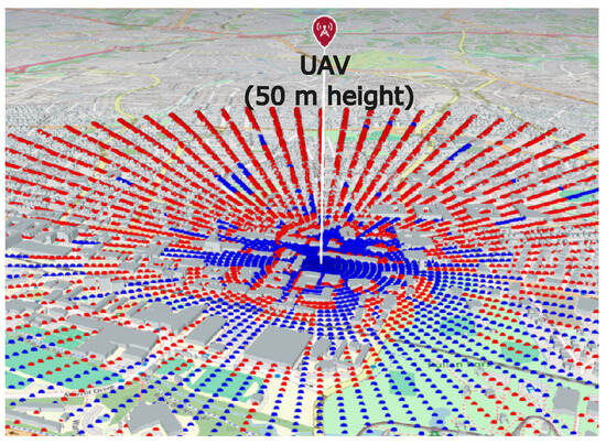
Figure 4.
A snapshot of visualized OSM 3-D map data by MATLAB Site Viewer, and LoS/NLoS condition analysis based on ray tracing where the color blue (red) indicates LoS (NLoS) links.
5.2. Realistic Antenna Designs
To consider realistic 3-D antenna patterns of dipole and downward directional antennas in ray tracing-based simulations, we design antennas utilizing antenna design tools in MATLAB. By configuring the length of the dipole antenna and the number of antenna elements in a uniform rectangular array (URA), we obtain antenna patterns with different beamwidth and directivity. The dipole antenna is modeled as a perfect electric conductor (PEC) without considering conductor losses. Figure 5 shows the 3-D realistic antenna patterns. The dipole antenna lengths are set to and , where denotes the wavelength. As shown in Figure 5c, the dipole with length exhibits a narrower beamwidth compared to the dipole with length . Furthermore, 4-by-4 (16 elements) and 6-by-6 (36 elements) URA arrays are configured to realize downward directional beamforming. Each array element is modeled as an isotropic radiator, and directional beam patterns are formed through phase-controlled beamforming. In addition, the spacing between antenna elements is set to , and Hamming tapering is applied to both URA antenna configurations. As shown in Figure 5d, the 4-by-4 URA exhibits a wider beamwidth than the 6-by-6 URA.
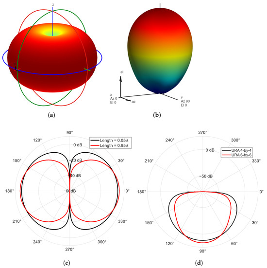
Figure 5.
Three-dimensional antenna patterns designed by the antenna design tool, where two different beamwidths are configured for both dipole and downward directional antennas: (a) 3-D dipole antenna pattern; (b) 3-D downward directional antenna pattern. (c) Two-dipole-antenna elevation patterns. (d) Two-downward-directional-antenna elevation patterns.
After obtaining the LoS/NLoS conditions of UEs through ray tracing analysis, the received signal power is calculated by (1), considering the configured realistic 3-D antenna patterns.
6. Numerical Results
In this section, we evaluate the simulation results of height-dependent UAV spectrum occupancy using both stochastic geometry-based closed-form analysis and realistic ray-tracing-based analysis.
6.1. Stochastic Geometry-Based Simulations
In this subsection, we present the simulation results to evaluate the analytical derivation of the aggregate received signal power depending on the receiver antenna setup and the UAV height. The simulation parameters are listed in Table 3.
Table 3.
Parameter setup of simulations.
Figure 6 shows the aggregate received signal power as a function of the UAV height with different parameter settings. We consider urban and suburban environments, different beamwidth , and two types of receiver antennas (the typical dipole antenna and the downward directional antenna). First, we observe that the closed-form analytical expressions and their convergence behaviors in Section 4 closely match Monte Carlo simulation results. Note that in Monte Carlo simulations, we directly use (2) and (5) without any approximations. Furthermore, we observe that the aggregate received signal power converges to a constant as the UAV altitude increases, which is consistent with the analytical results in Remark 3 and Equation (18).
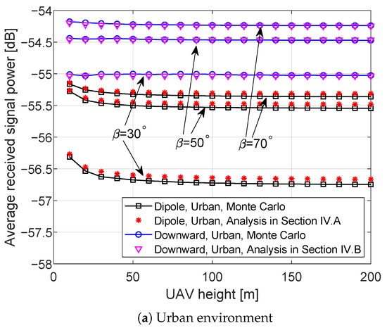
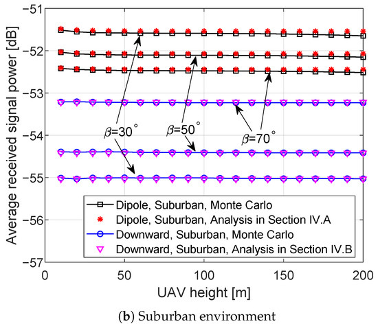
Figure 6.
Average aggregate received signal power depending on the UAV height where the Monte Carlo and analytical results are overlapped with different receiver antennas and the type of environments, and .
It is also observed that (1) the average aggregate signal power in suburban contexts is higher than that in urban contexts, especially for the typical dipole antenna; (2) in urban contexts, wider beamwidth provides higher signal power with both the typical dipole and the downward directional antennas; (3) in suburban contexts, wider beamwidth provides higher signal power with the downward directional antenna but lower signal power with the typical dipole antenna; (4) the decrease in average aggregate signal power at low height is more significant in urban environments and for the typical dipole antenna compared to suburban environments and the downward directional antenna. In addition, our analytical model does not account for shadowing effects, which may contribute additional fluctuations to the aggregate received signal.
6.2. Ray Tracing-Based Simulations
In this subsection, we present the ray tracing-based simulation results discussed in Section 5. The simulation results in Section 6.1 focus on the mathematical models based on a stochastic geometry framework, while ray tracing results consider the real-world 3-D map and realistic 3-D antenna pattern designs to evaluate the height-dependent spectrum occupancy in practical environments.
Figure 7 illustrates the average received signal power versus UAV height based on ray-tracing simulations. Two antenna configurations shown in Figure 5—a dipole and a downward directional antenna—are employed, considering relatively wide and narrow beamwidths, respectively. The results show that the average received signal power gradually decreases and converges to a constant value as the UAV height increases. Compared with the stochastic geometry-based results in Figure 6, the decreasing trend is clear but converges more slowly. This discrepancy between stochastic geometry analysis and ray-tracing simulation arises from several factors: the difference between Poisson point process (PPP)-based UE deployment and fixed-grid deployment, the use of rectangular antenna models versus realistic antenna patterns, the difference between the statistical LoS probability function and the deterministic LoS/NLoS conditions computed from real-world 3D building geometry, and the limited radius of area (2 km) on the ray tracing simulation environment. Among these factors, the difference in the convergence slope primarily stems from the mismatch between the statistical LoS probability model in (5) and the actual building layout and height distribution in the real-world map used for ray tracing. Furthermore, as the beamwidth of the dipole antenna patterns becomes narrower, the average received signal power decreases, and the average received signal power achieved with the downward directional antenna is higher than that with the dipole antenna, which is consistent with the stochastic model-based results obtained for the urban environment in Figure 6a.
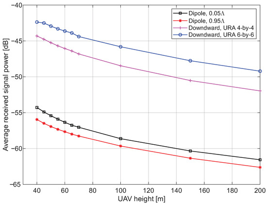
Figure 7.
Average aggregate received signal power based on the ray tracing-based simulations discussed in Section 5. LoS/NLoS status is obtained by a real-world 3-D map, and realistic dipole and downward directional antennas are adopted.
7. Concluding Remark
In this paper, we study UAV height-dependent cellular spectrum occupancy by analyzing the impact of different receiver antenna types and beamwidth configurations. A closed-form analytical framework is developed based on the HPPP model, the LoS probability function, and 3D antenna radiation pattern models. The analytical results are validated through Monte Carlo simulations. In addition, to evaluate the height-dependent spectrum occupancy trend in a practical environment, we consider ray tracing-based analysis considering real-world 3-D map data and realistic 3-D antenna pattern designs. We characterize the altitude-dependent occupancy behavior by analyzing the aggregate received signal power, which exhibits asymptotic convergence with increasing UAV height. Simulation results further demonstrate how environmental conditions, antenna type, and beamwidth shape the UAV’s spectrum occupancy performance.
From a practical perspective, these results imply that UAVs experience relatively stable spectrum occupancy levels at altitudes above approximately 200 m, though this threshold may vary depending on environmental conditions such as urban or suburban settings, making such flight altitudes more suitable for long-range communication or sensing missions. Furthermore, antenna design and beamwidth configuration should be carefully optimized depending on the operating environment. As future research directions, extending the analysis to adaptive or dynamic beam steering scenarios, as well as to cooperative multi-UAV sensing and communication frameworks, would provide valuable insights for designing efficient 3D aerial networks.
Funding
This work was supported by the research fund of Hanyang University (HY-2025-2756).
Data Availability Statement
The original contributions presented in this study are included in the article. Further inquiries can be directed to the corresponding author.
Conflicts of Interest
The author declares no conflict of interest.
References
- Xiao, Z.; Dong, H.; Bai, L.; Wu, D.O.; Xia, X.G. Unmanned aerial vehicle base station (UAV-BS) deployment with millimeter-wave beamforming. IEEE Internet Things J. 2020, 7, 1336–1349. [Google Scholar] [CrossRef]
- Zhang, C.; Zhang, L.; Zhu, L.; Zhang, T.; Xiao, Z.; Xia, X.G. 3D deployment of multiple UAV-mounted base stations for UAV communications. IEEE Trans. Commun. 2021, 69, 2473–2488. [Google Scholar] [CrossRef]
- Shang, B.; Marojevic, V.; Yi, Y.; Abdalla, A.S.; Liu, L. Spectrum sharing for UAV communications: Spatial spectrum sensing and open issues. IEEE Veh. Technol. Mag. 2020, 15, 104–112. [Google Scholar] [CrossRef]
- Maeng, S.J.; Ozdemir, O.; Güvenç, İ.; Sichitiu, M.L. Kriging-based 3-D spectrum awareness for radio dynamic zones using aerial spectrum sensors. IEEE Sens. J. 2024, 24, 9044–9058. [Google Scholar] [CrossRef]
- Namuduri, K.; Fiebig, U.C.; Matolak, D.W.; Guvenc, I.; Hari, K.; Määttänen, H.L. Advanced air mobility: Research directions for communications, navigation, and surveillance. IEEE Veh. Technol. Mag. 2022, 17, 65–73. [Google Scholar] [CrossRef]
- Guo, J.; Chen, L.; Li, L.; Na, X.; Vlacic, L.; Wang, F.Y. Advanced air mobility: An innovation for future diversified transportation and society. IEEE Trans. Intell. Veh. 2024, 9, 3106–3110. [Google Scholar] [CrossRef]
- Peng, Y.; Xiang, L.; Yang, K.; Jiang, F.; Wang, K.; Wu, D.O. SIMAC: A Semantic-Driven Integrated Multimodal Sensing And Communication Framework. IEEE J. Sel. Areas Commun. 2025. [Google Scholar] [CrossRef]
- Zhou, S.; Xiang, L.; Yang, K.; Wong, K.K.; Wu, D.O.; Chae, C.B. Beamforming-based achievable rate maximization in ISAC system for multi-UAV networking. arXiv 2025, arXiv:2507.21895. [Google Scholar]
- Raouf, A.H.F.; Maeng, S.J.; Guvenc, I.; Özdemir, Ö.; Sichitiu, M. Spectrum monitoring and analysis in urban and rural environments at different altitudes. In Proceedings of the IEEE 97th Vehicular Technology Conference, Florence, Italy, 20–23 June 2023; pp. 1–7. [Google Scholar] [CrossRef]
- Azari, M.M.; Rosas, F.; Chiumento, A.; Ligata, A.; Pollin, S. Uplink performance analysis of a drone cell in a random field of ground interferers. In Proceedings of the IEEE Wireless Communications and Networking Conference, Barcelona, Spain, 15–18 April 2018; pp. 1–6. [Google Scholar] [CrossRef]
- Banagar, M.; Chetlur, V.V.; Dhillon, H.S. Stochastic geometry-based performance analysis of drone cellular networks. In UAV Communications for 5G and Beyond; John Wiley & Sons Ltd.: Hoboken, NJ, USA, 2020; pp. 231–254. [Google Scholar] [CrossRef]
- Matracia, M.; Kishk, M.A.; Alouini, M.S. UAV-aided post-disaster cellular networks: A novel stochastic geometry approach. IEEE Trans. Veh. Technol. 2023, 72, 9406–9418. [Google Scholar] [CrossRef]
- Ravi, V.V.C.; Dhillon, H.S. Downlink coverage probability in a finite network of unmanned aerial vehicle (UAV) base stations. In Proceedings of the IEEE International Workshop on Signal Processing Advances in Wireless Communications, Edinburgh, UK, 3–6 July 2016; pp. 1–5. [Google Scholar] [CrossRef]
- Maeng, S.J.; Raouf, A.H.F.; Ozdemir, O.; Zajkowski, T.; Mushi, M.; Sichitiu, M.L.; Dutta, R.; Guvenc, I. Altitude-Dependent Sub-6 GHz Wireless Spectrum: Survey, Measurements, Trends, and Modeling. TechRxiv 2025. [Google Scholar] [CrossRef]
- Maeng, S.J.; Ozdemir, O.; Güvenç, İ.; Sichitiu, M.L.; Mushi, M.; Dutta, R.; Ghosh, M. SDR-based 5G NR C-band i/q monitoring and surveillance in urban area using a helikite. In Proceedings of the IEEE International Conference on Industrial Technology (ICIT), Orlando, FL, USA, 4–6 April 2023; pp. 1–6. [Google Scholar] [CrossRef]
- Maeng, S.J.; Guvenc, I. Altitude-Dependent Cellular Spectrum Occupancy: From Measurements to Stochastic Geometry Models. IEEE Internet Things J. 2025, 12, 30268–30281. [Google Scholar] [CrossRef]
- Matolak, D.W.; Sun, R. Unmanned Aircraft Systems: Air-Ground Channel Characterization for Future Applications. IEEE Veh. Technol. Mag. 2015, 10, 79–85. [Google Scholar] [CrossRef]
- Yanmaz, E.; Kuschnig, R.; Bettstetter, C. Achieving air-ground communications in 802.11 networks with three-dimensional aerial mobility. In Proceedings of the IEEE INFOCOM, Turin, Italy, 14–19 April 2013; pp. 120–124. [Google Scholar] [CrossRef]
- Feng, Q.; Tameh, E.K.; Nix, A.R.; McGeehan, J. WLCp2-06: Modelling the Likelihood of Line-of-Sight for Air-to-Ground Radio Propagation in Urban Environments. In Proceedings of the IEEE Globecom, San Francisco, CA, USA, 27 November–1 December 2006; pp. 1–5. [Google Scholar] [CrossRef]
- Al-Hourani, A.; Kandeepan, S.; Lardner, S. Optimal LAP altitude for maximum coverage. IEEE Wireless Commun. Lett. 2014, 3, 569–572. [Google Scholar] [CrossRef]
- ITU. Rec. P.1410 Propagation Data and Prediction Methods Required for the Design of Terrestrial Broadband Millimetric Radio Access Systems Operating in a Frequency Range of About 20–50 GHz. P Series, Radiowave Propagation. 2003. Available online: https://www.itu.int/rec/R-REC-P.1410 (accessed on 1 November 2025).
- ElSawy, H.; Sultan-Salem, A.; Alouini, M.S.; Win, M.Z. Modeling and analysis of cellular networks using stochastic geometry: A tutorial. IEEE Commun. Surv. Tuts. 2017, 19, 167–203. [Google Scholar] [CrossRef]
- Balanis, C.A. Antenna Theory: Analysis and Design; John Wiley & Sons: Hoboken, NJ, USA, 2015. [Google Scholar]
- OpenStreetMap. Available online: https://www.openstreetmap.org/ (accessed on 1 November 2025).


Disclaimer/Publisher’s Note: The statements, opinions and data contained in all publications are solely those of the individual author(s) and contributor(s) and not of MDPI and/or the editor(s). MDPI and/or the editor(s) disclaim responsibility for any injury to people or property resulting from any ideas, methods, instructions or products referred to in the content. |
© 2025 by the author. Licensee MDPI, Basel, Switzerland. This article is an open access article distributed under the terms and conditions of the Creative Commons Attribution (CC BY) license (https://creativecommons.org/licenses/by/4.0/).