Highlights
What are the main findings?
- Green and Red bands proved to be particularly effective for detecting plastics in freshwater environments.
- The proposed Plastic Detection Index (PDI) and Heterogeneity Plastic Index (HPI) enhanced the discrimination of plastics from water and vegetation.
What are the implications of the main findings?
- UAV-based multisensor systems represent a cost-effective solution for high-resolution monitoring of plastic pollution in inland waters.
- The methodology can be scaled to different aquatic environments and integrated into automated classification frameworks to support environmental monitoring programs.
Abstract
This study addresses the observation of floating plastic debris in freshwater environments using an Unmanned Aerial Vehicle (UAV) multi-sensor strategy. An experimental campaign is described where an heterogeneous plastic assemblage, namely a plastic target, and a naturally occurring leaf-litter mat are observed by a UAV platform in the Lake Calore (Avellino, Southern Italy) within the framework of the “multi-layEr approaCh to detect and analyze cOastal aggregation of MAcRo-plastic littEr” (ECOMARE) Italian Ministry of Research (MUR)-funded project. Three UAV platforms, equipped with optical, multispectral, and thermal sensors, are adopted, which overpass the two targets with the objective of analyzing the sensitivity of optical radiation to plastic and the possibility of discriminating the plastic target from the natural one. Georeferenced orthomosaics are generated across the visible, multispectral (Green, Red, Red Edge, Near-Infrared—NIR), and thermal bands. Two novel indices, the Plastic Detection Index (PDI) and the Heterogeneity Plastic Index (HPI), are proposed to discriminate between the detection of plastic litter and natural targets. The experimental results highlight that plastics exhibit heterogeneous spectral and thermal responses, whereas natural debris showed more homogeneous signatures. Green and Red bands outperform NIR for plastic detection under freshwater conditions, while thermal imagery reveals distinct emissivity variations among plastic items. This outcome is mainly explained by the strong NIR absorption of water, the wetting of plastic surfaces, and the lower sensitivity of the Mavic 3′s NIR sensor under high-irradiance conditions. The integration of optical, multispectral, and thermal data demonstrate the robustness of UAV-based approaches for distinguishing anthropogenic litter from natural materials. Overall, the findings underscore the potential of UAV-mounted remote sensing as a cost-effective and scalable tool for the high-resolution monitoring of plastic pollution over inland waters.
1. Introduction
Aquatic systems, including oceans, rivers, and lakes, are fundamental components of the Earth system. They regulate the global climate, sustain biodiversity, and provide critical ecosystem services such as food supply, oxygen production, and carbon storage. However, these environments are increasingly exposed to anthropogenic pressures, among which plastic pollution has emerged as one of the most pervasive threats. Plastics account for nearly 80% of marine debris worldwide [1], with an estimated 11–14 million tons entering the oceans every year [2,3,4], either directly from coastal activities or indirectly through rivers and drainage networks [5].
Unlike organic material, plastics are not biodegradable and they persist in the environment for centuries. Larger items fragment into progressively smaller particles, namely microplastics, which are often invisible to the human eye but can be ingested by aquatic organisms, leading to intestinal blockages, malnutrition, and even mortality [6,7,8]. These particles also bioaccumulate along food webs, ultimately reaching humans and raising significant concerns regarding their potential health impacts [9,10]. Recent studies indicate that global plastic production now exceeds 400 million tons annually, with no sign of decline [11]. Without effective mitigation strategies, projections suggest that by 2050 the mass of plastic in the oceans could surpass that of fish [12].
Plastic pollution monitoring is an intrinsically multidisciplinary and challenging task, involving waste management, production analysis, and environmental observation. In this context, remote sensing has gained increasing attention due to its capacity to monitor large or inaccessible areas across multiple spatial and temporal scales [13]. Various platforms have been employed, from satellites and aircraft to Unmanned Aerial Vehicles (UAVs, or drones), each offering specific advantages depending on the monitoring objectives.
Passive optical remote sensing is widely applied for the detection of floating debris, leveraging the characteristic spectral reflectance and absorption features of plastics across the visible to short-wave infrared (VIS–SWIR) range [14,15]. Multispectral and hyperspectral imaging, both satellite and proximity-based, have proven to be effective for discriminating plastics from their surroundings [16,17,18], with hyperspectral data enabling fine-scale identification based on detailed spectral signatures [19,20,21]. Nevertheless, optical techniques are highly dependent on atmospheric conditions and solar illumination, which can reduce their reliability under cloudy skies, during low-light conditions, or at night.
To complement these limitations, thermal infrared sensing has been proposed as an alternative or synergistic tool. Plastics and surrounding water often exhibit measurable thermal contrasts, enabling detection even in the absence of sunlight and potentially reducing confusion with natural floating materials such as vegetation or foam [22,23].
Active remote sensing further expands these capabilities. Light Detection and Ranging (LiDAR), for example, can exploit material-dependent fluorescence properties to distinguish plastics from organic matter [24,25,26,27,28], while the Synthetic Aperture Radar (SAR) offers all-weather, day–night imaging capabilities in the microwave electromagnetic range and has often been used for detecting pollution at sea [27,28,29]. However, SAR applications for plastic detection remain challenging due to the low plastic reflectivity in the microwave range of the spectrum and the mismatch between radar wavelengths and the dimensions of microplastics [30,31,32,33,34].
Although satellite sensors provide global coverage, airborne platforms and UAVs offer significantly higher spatial resolution, which is essential for identifying small-scale litter aggregations and mapping debris hotspots [35,36,37,38,39,40]. To overcome the limitations of single-sensor approaches, recent research increasingly emphasizes multisensor integration, where optical, thermal, and other sensing modalities are combined to maximize detection performance and reliability [41,42,43,44,45]. These approaches are typically validated in field experiments or controlled environments that replicate real-world aquatic conditions [46,47,48,49].
In this context, the development of indices able to detect plastic has been achieved, through the use of optical [14,50] and superspectral [51] data. Furthermore, plastic detection on beaches has been accomplished using the method proposed by [52].
Building on this framework, this study summarizes results from an experimental campaign conducted within the research project “multi-layEr approaCh to detect and analyze cOastal aggregation of MAcRo-plastic littEr” (ECOMARE), funded by the Italian Ministry of University and Research [45,53]. A plastic target (2 m × 2 m) composed of heterogeneous synthetic materials representative of macroplastic litter was deployed on Lake Calore (Italy), on which a natural target consisting of leaf waste also floated. Three UAV platforms equipped with complementary sensors, namely an optical visible (or RGB, Red–Green–Blue) camera, a multispectral camera, and a thermal infrared sensor, were employed to assess their individual and combined potential for plastic detection.
The objectives of this work are twofold: (i) to analyze the spectral and thermal response of floating plastics and discuss their differences with respect to natural material; (ii) to evaluate the strengths and limitations of UAV-based optical, multispectral, and thermal imaging for detecting and characterizing plastic debris over inland waters. This piece of research aims to contribute to the development of integrated remote sensing strategies for the high-resolution monitoring of plastic pollution in aquatic environments.
2. Materials and Methods
The methodological framework to evaluate the performance of different UAV-mounted sensors in detecting and characterizing floating macroplastic litter under controlled but realistic conditions is described here. A dedicated in situ campaign was conducted on Lake Calore, where both plastic and natural floating targets were surveyed. Data acquisition was performed using three UAV platforms equipped with optical, multispectral, and thermal sensors, enabling a multi-perspective analysis of the same scene.
The workflow consists of three main steps: (i) preparation of targets and UAV-based data collection, (ii) photogrammetric processing for the generation of georeferenced orthomosaics in RGB, multispectral, and thermal domains, and (iii) spectral and thermal analyses to discuss the how to discern plastic debris from natural organic matter.
2.1. Test Site and Experimental Setup
The experimental survey was carried out on Lake Calore (Mirabella Eclano, Avellino, Southern Italy) on 31 July 2024. The site was selected for its calm water conditions and limited anthropogenic disturbance, which make it a controlled environment when discussing the sensitivity of UAV platforms to plastic and natural litter.
Two distinct floating targets are discussed:
- Plastic Target (see Figure 1): A 2 × 2 m floating platform composed of heterogeneous plastic items, such as bottles, containers, and polystyrene (white or graphite), distributed over a supporting structure built from plastic tubing. The structure is anchored to the lake shores with four ropes to ensure stability during aerial data acquisitions. This plastic target is expected to mimic the behavior of floating aggregated plastic litter.
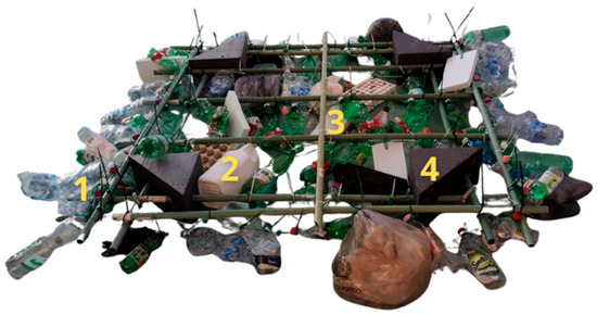 Figure 1. Plastic target used in the experimental campaign, composed of bottles (1), containers (2), and polystyrene blocks, which are either white (3) or graphite (4).
 - Natural Target: An almost 5 m diameter compact aggregation of floating leaves and plant debris, naturally accumulated along the shore of the lake. The natural target is used to test the ability of UAV platforms to discriminate the plastic target from natural litter.
2.2. UAV Platforms and Sensors
Three DJI Mavic 3 series UAVs were employed, each equipped with a different payload to provide complementary information, as detailed in Table 1. All UAVs were equipped with Real-Time Kinematic (RTK) modules, enabling centimeter-level geolocation accuracy by receiving differential corrections from the GRO1 Global Navigation Satellite System (GNSS) station of the INGV permanent GNSS network [54,55], located in Grottaminarda (Italy), serving as the base station for RTK corrections.

Table 1.
Technical specifications of the UAV platforms and sensors employed in the experimental campaign.
2.3. Flight Planning and Data Acquisition
Flights were performed on 31 July 2024 at 11:00 UTC, under clear sky and low wind conditions (<2 m/s). To ensure systematic and repeatable data acquisition from UAVs, the flight mission was planned and executed using UgCS Enterprise v 4.22 (Universal Ground Control) Software. This software allows for a detailed configuration of flight parameters, including altitude, front and side overlap, flight speed, and the flight path itself, as resumed in Table 2. The mission is designed to fly at a constant flight altitude of 15 m AGL (Above Ground Level) and with an 80% front and side overlap, ensuring optimal photogrammetric coverage. The flight path is designed to fully cover the water surface area, containing both artificial and natural targets, with evenly spaced waypoints and parallel flight lines.
Table 2.
Flight mission information of the UAV survey over Lake Calore.
During the experimental campaign, the DJI Mavic 3 platforms (Enterprise, Multispectral, and Thermal) adopted the predefined plan autonomously. Camera triggering was automatically managed at each waypoint, ensuring consistent spatial resolution and coverage across the different sensors.
2.4. Photogrammetric Processing
Raw images were processed in Agisoft Metashape Professional version 2.0 using a Structure-from-Motion (SfM) workflow:
- Image alignment and sparse point cloud generation;
- Dense point cloud reconstruction;
- Production of orthomosaics in RGB, multispectral, and thermal domains.
These orthomosaics are geometrically corrected to eliminate distortions and to provide the basis for subsequent analyses.
A total of 152 RGB, 120 multispectral, and 96 thermal images were processed. Multispectral data were radiometrically corrected through dark offset removal and reflectance normalization using the integrated irradiance sensor of the DJI Mavic 3 Multispectral. The resulting orthomosaics achieved Root Mean Square Errors (RMSE) of 0.021 m (RGB), 0.034 m (Multispectral), and 0.041 m (Thermal), ensuring high geometric consistency across datasets. The final orthomosaic resolutions were 1.49 cm/pixel, 5.0 cm/pixel, and 6.2 cm/pixel, respectively.
2.5. Optical Analysis
The RGB imagery collected by the DJI Mavic 3 Enterprise were processed to produce a high-resolution orthomosaic with a ground sampling distance (GSD) of 1.5 cm/pixel. This serves as the reference base map for geolocating the plastic and natural targets, as shown in Figure 2.
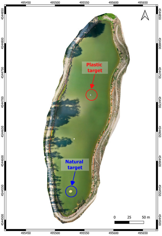
Figure 2.
High-resolution optical orthomosaic of the Lake Calore test site. The plastic and natural targets are enclosed in red and blue circles, respectively.
Two main targets were identified (see Section 2.1):
- The plastic target, situated in the central–northern region of the lake, which is marked by a red circle;
- A natural target, situated near the southern shore of the lake, which is marked by a blue circle.
2.6. Multispectral Pre-Processing
Multispectral imagery collected by Mavic 3 Multispectral is radiometrically corrected and normalized (Equation (1)). For each band, digital numbers (DN) were rescaled to a [0–1] range:
This normalization enables direct comparison among bands. In a further step, spectral indices based on custom band combinations are derived to enhance discrimination between plastic, water, and natural debris.
2.7. Thermal Pre-Processing
Thermal acquisitions collected by Mavic 3 Thermal were obtained simultaneously with optical and multispectral flights. Unlike typical night-time thermal surveys, this experiment was performed during daytime (ascending solar heating phase). This setup allows for plastic detection performance to be evaluated under more challenging but operationally relevant conditions.
Thermal orthomosaics were analyzed to achieve the following:
- Assess temperature contrasts between plastics, water, and natural debris;
- Evaluate intra-target variability among different plastic subtypes;
- Test the relative homogeneity of the natural reference target.
3. Results
3.1. Optical Results
To enable a quantitative analysis, reference transects were considered across both targets, as shown by the lines in Figure 3. For the plastic target, four transects were defined to capture the internal heterogeneity of the deployed structure: A–A′ and B–B′ (north–south orientation) and C–C′ and D–D′ (east–west orientation); see Figure 3a. For the natural target, which exhibits a more homogeneous distribution, two orthogonal transects were drawn: E–E′ (north–south) and F–F′ (west–east); see Figure 3b. These transects provide spatially consistent references for subsequent spectral and radiometric analyses.
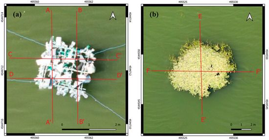
Figure 3.
High-resolution optical orthomosaic over the plastic (a) and the natural (b) target. Reference transects selected for the quantitative analysis are also annotated as red lines.
Figure 4 shows the optical reflectance profiles for the three visible bands (Red, Green, and Blue) along the transects crossing the plastic target.
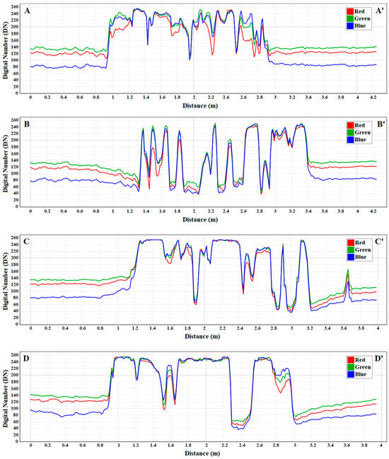
Figure 4.
Optical response of red (red curve), green (green curve), and blue (blue curve) bands evaluated along the transects (A–A′, B–B′, C–C′, D–D′) excerpted over the area affected by the plastic target; see Figure 3a. The x-axis represents the distance in meters along each profile, and the y-axis shows the reflectance values in DN.
The initial and final sections of the profiles, corresponding to open water, show stable and uniform values, with the Blue band being consistently less reflective than the Red and Green.
The central part of the curves is related to the plastic-affected area, which results in a reflectance value showing remarkable heterogeneity, with sharp peaks approaching values of 260. These fluctuations reflect the variable spectral responses of the heterogeneous plastic composition, encompassing different materials, colors, and surfaces.
In Figure 5, the transect analysis that refers to the natural target, see Figure 3b, is depicted, showing the reflectance profiles along transects E–E′ and F–F′. In this case, a more homogeneous spectral behavior is obtained: the Red and Green bands maintain stable high values, while the Blue band remains consistently lower. Oscillations are smoother and more regular than those of the plastic target.
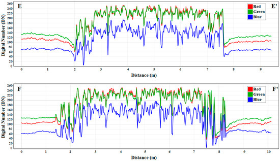
Figure 5.
Optical response in the red (red curve), green (green curve) and blue (blue curve) bands evaluated along the transects (E–E′ and F–F′) excerpted on the natural target. The x-axis represents the distance in meters along each profile, while the y-axis shows the reflectance values in DN.
This behavior is consistent with the uniform reflectance of decomposed leaf litter and natural organic matter [56,57,58].
3.2. Multispectral Results
In Figure 6a–d the orthomosaics of the plastic target in the Green, Red, Red Edge, and NIR bands are depicted, respectively.
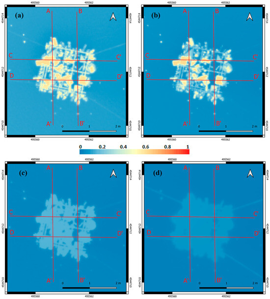
Figure 6.
Multispectral images of the plastic target, evaluated in the Green (a), Red (b), Red Edge (c) and NIR (d) bands.
In the Green band, see Figure 6a, the plastic target appears as a patchwork of bright and dark areas, with several zones exceeding reflectance values of 0.6. The brightest responses result from the white and graphite polystyrene components (labels 3 and 4 in Figure 1), which are easily distinguishable from both surrounding water and other plastic items, such as bottles and containers, whose reflectance is generally lower. The Red band (Figure 6b) reveals a similar pattern, with sharp boundaries and spatially coherent bright spots highlighting the internal heterogeneity of the plastic assemblage.
In contrast, the Red Edge and NIR images, see Figure 6c,d, respectively, show a significantly lower reflectance, rarely exceeding 0.4, and with the plastic resulting in quite homogeneous reflectance values, which are higher than the surrounding water. This is in contrast with the literature studies [14,15,50], where the NIR band is often considered to be optimal for plastic detection due to the large contrast between plastic and seawater. However, most of these studies relied on satellite-borne instruments, which operate at coarser spatial resolutions and under different observation and illumination conditions than UAV-based systems. This highlights the importance of acquisition context when selecting effective spectral domains for plastic identification.
In addition, although water exhibits strong absorption at NIR [59] almost independently of turbidity or salinity, which have a negligible effect at these wavelengths [60,61,62], the reduction in plastic reflectance in the NIR band due to the wetness of the plastic conditions has been demonstrated in [49]. This effect is therefore likely to explain the results observed in our study.
On the other side, in the visible range, wetness has little effect on reflectance because water absorption is still relatively low [63]. Similarly, experiments in [64] show how plastics reflectance varies according to surface conditions (dry, wet, or submerged), confirming that immersion strongly attenuates the measurable NIR signal.
From an instrumental perspective, the DJI Mavic 3 Multispectral employs compact 1/2.8″ and 5-megapixel CMOS sensors, where each pixel collects a limited amount of light. In the case of plastic targets that are submerged in water or wet, the reflected NIR signal is already weak due to the strong water absorption at these wavelengths. Consequently, only a small portion of radiance reaches the detector, while the electronic noise of the sensor remains constant, leading to a low signal-to-noise ratio (SNR). Conversely, in the red and green bands, where water absorption is lower and illumination is higher, the reflected signal remains strong and the plastic is more easily distinguishable.
Finally, the measurements were conducted around solar noon under clear-sky conditions, when high solar elevation angles enhance specular reflection (sun-glint) on the water surface. This effect can increase the apparent reflectance in the visible bands while further attenuating NIR contributions [65,66,67].
The combination of these factors—optical absorption by water, wetting of the plastic surface, sensor SNR limitations, and illumination geometry—supports our experimental findings, which show a higher reflectance observed in the visible spectrum compared to the NIR.
The quantitative analysis, which consists of discussing the behavior of the transects extracted over the plastic target, is provided in Figure 7, confirming the qualitative analysis. In the water section of each transect, all four bands remain flat and close to zero, as expected for freshwater.
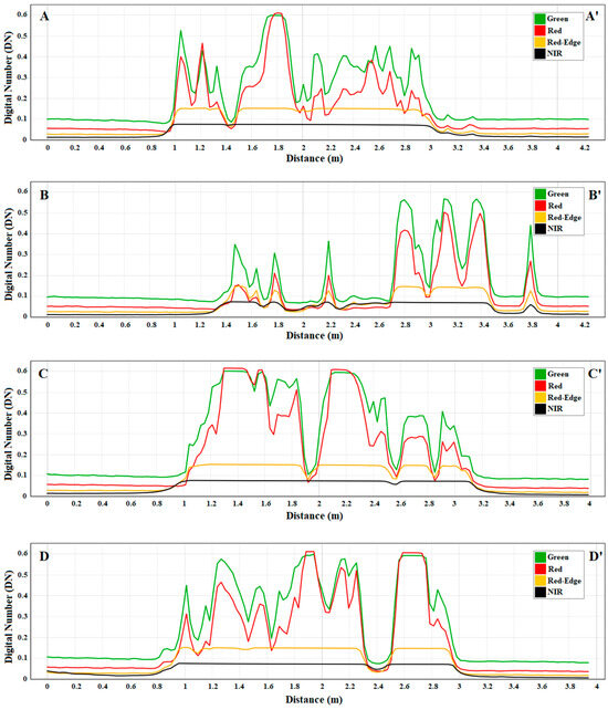
Figure 7.
Multispectral response of green (green curve), red (red curve), red edge (orange curve) and NIR (black curve) bands evaluated along the transects (A–A′, B–B′, C–C′, D–D′) excerpted on the plastic target. The x-axis represents the distance in meters along each profile, and the y-axis shows the reflectance values in DN.
Within the central parts crossing the plastic structure, the Green (green curve) and Red (red curve) bands show a pronounced variability, with frequent peaks up to 0.6 and abrupt drops between adjacent materials. These oscillations reflect the heterogeneous composition of the plastic target, made up of objects differing in size, color, and surface properties. In contrast, the Red Edge (orange curve) and NIR (black curve) bands remain consistently lower, rarely exceeding 0.2, and exhibit a relatively flat trend, underscoring their limited ability to discriminate among the different plastic types under these conditions.
The natural target presents a markedly different behavior, as shown in Figure 8, which illustrates the multispectral orthomosaics of the vegetation mat.
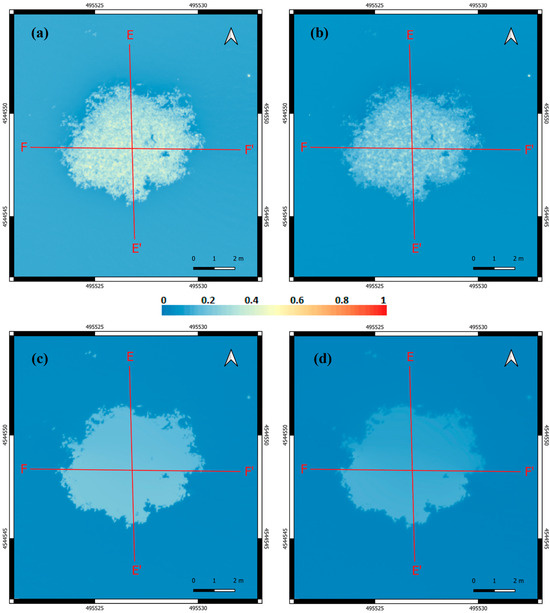
Figure 8.
Multispectral orthomosaic focused on the natural target, evaluated in the Green (a), Red (b), Red Edge (c) and NIR (d) bands.
In the Green and Red bands, see Figure 8a,b, respectively, the target appears homogeneous, with reflectance values generally between 0.3 and 0.6. The reflectance resulting from the target exhibits a smooth spatial variability. The natural target exhibits a larger reflectance value than the plastic one in the Red Edge (Figure 8c) and NIR (Figure 8d) bands. This behavior is consistent with the spectral properties of photosynthetically active material, which reflects strongly in these domains due to the presence of chlorophyll and other pigments [68,69,70].
The quantitative analysis, carried out by evaluating the reflectance values along with the transects of Figure 3, is depicted in Figure 9, which supports the qualitative visual interpretation. In both transects E–E′ and F–F′, the Green and Red curves are the most reflective, showing smooth and stable patterns with only minor oscillations. The Red Edge and NIR curves, while lower in magnitude, are continuous and regular, with values typically between 0.15 and 0.25. Unlike the plastic target, no sharp peaks or abrupt changes are observed, confirming the homogeneous and compact nature of the vegetation mass.
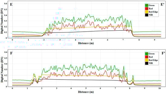
Figure 9.
Multispectral reflectance values evaluated along with the transects (E–E′, F–F′) excerpted over the of green (green curve), red (red curve), red edge (orange curve) and NIR (black curve) bands of the image related to the natural target. The x-axis represents the distance in meters along each profile, and the y-axis shows the reflectance values in DN.
The quantitative multispectral reflectance analysis is summarized in Table 3, which reports, for each spectral band, the reflectance range, expressed by the mean (μ) and standard deviation (σ) values, and the coefficient of variation (CV%), calculated as the ratio between the standard deviation and the mean (σ/μ) and expressed as a percentage. These parameters were obtained by averaging the reflectance of the pixels corresponding to the three materials—plastic, natural, and water—previously isolated along each transect.
Table 3.
Reflectance mean (μ), standard deviation (σ) and coefficient of variation (CV%) of multispectral bands measured for water, natural, and plastic materials.
The following conclusions can be drawn: (a) plastic litter consistently reflects more strongly than water in the Green and Red bands, making these channels particularly effective for separating synthetic debris from the aquatic background; (b) plastic litter reflects more strongly than the natural target in the visible spectrum, with larger (but fluctuating) reflectance values; (c) natural targets dominate the Red Edge and NIR reflectance, resulting in slightly higher values than those of plastic debris. This behavior is consistent with the presence of photosynthetically active pigments.
3.3. Multispectral Indices
To enhance the possibility of detecting aggregated plastics with respect to the surrounding water and distinguishing the synthetic debris from the accumulated natural debris, two novel indexes are introduced here: the Plastic Detection Index (PDI) and the Heterogeneity Plastic Index (HPI). Both indices are calculated using normalized multispectral bands to allow for comparison across a consistent 0–1 range.
- Plastic Detection Index:
The PDI is designed to maximize the contrast between plastics and water by exploiting the Green and Red bands (Equation (2)), which, in the sensitivity analysis, were shown to have the strongest discrimination ability. The PDI is defined as follows:
The orthomosaic built using the PDI is depicted in Figure 10, which clearly differentiates the plastic target (see Figure 10a) from the natural one (see Figure 10b).
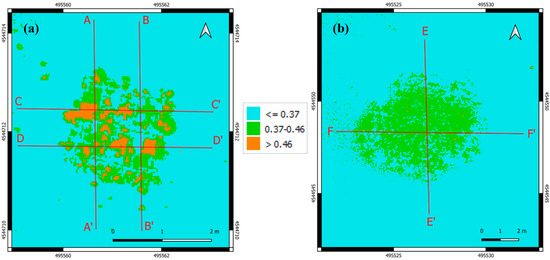
Figure 10.
PDI orthomosaic image excerpted over the plastic target (a) and the natural target (b).
Three classes were defined based on the empirical observation of index values in the orthomosaic. Thresholds were set to highlight the differences between water, vegetation and plastic.
In the case of the plastic target, the PDI exhibits a quite heterogeneous spatial pattern showing the areas with the highest reflectance (>0.46); areas with intermediate values (0.37–0.46); and areas resulting with a reflectance that is indistinguishable from that of water. This fragmented spatial pattern mirrors the heterogeneity of the plastic materials deployed. Bright plastics, such as white and graphite polystyrene, consistently return high index values, while darker or partially submerged plastics generate intermediate responses. In addition, since the plastic target is not completely filled with plastic material, holes are produced in which the reflectance of water prevails. This patchy but distinct behavior creates a clear contrast with the surrounding water, which appears uniform in the lowest class (≤0.37).
By contrast, the natural target shows a much more uniform spatial pattern in terms of the PDI values, which mostly belong to the intermediate range (0.37–0.46). This homogeneous spatial pattern is consistent with the stable spectral response of decomposed floating vegetation. However, it also implies that, in this intermediate range, plastic material (especially darker plastic) results in PDI values that partially overlap with those of the natural targets.
These qualitative analyses were confirmed by the quantitative analysis performed by evaluating PDI along with the transects (A–A′, B–B′, C–C′, D–D′) related to the plastic target; see Figure 11.
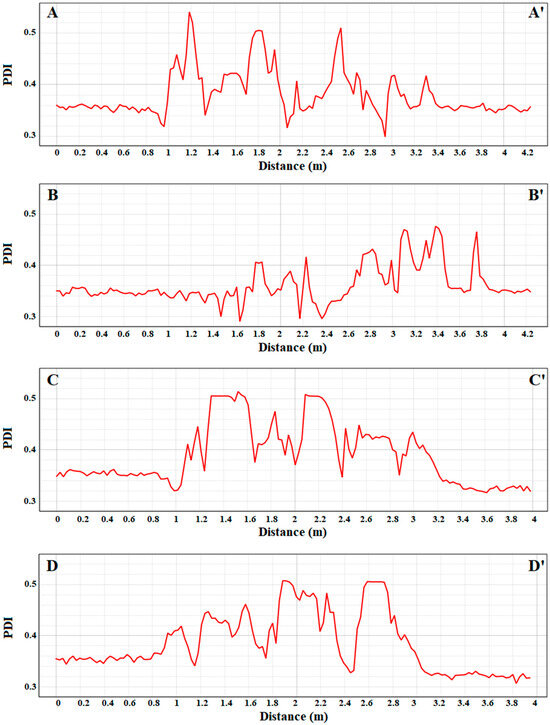
Figure 11.
PDI evaluated along the transects (A–A′, B–B′, C–C′, D–D′) excerpted along with the plastic target. The x-axis represents the distance in meters along each profile, and the y-axis shows the values of the PDI.
It can be noted that several sharp peaks appear in the PDI values, which are often above 0.46. These peaks alternate with sudden drops, corresponding to transitions between different plastic components, and reflect the strong internal variability of the target. This result reveals a largely irregular pattern in the central portions where plastics are concentrated.
The same transect analysis is depicted, for the natural target, in Figure 12, where transects E–E′ and F–F′ are shown.
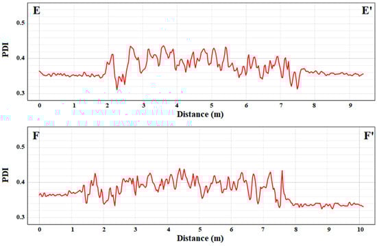
Figure 12.
PDI values evaluated, along with the two transects (E–E′, F–F′) excerpted over the natural target. The x-axis represents the distance in meters along each profile, and the y-axis shows the values of the PDI.
The PDI values still suggest smoother variability, placing them within the intermediate range of 0.37–0.46. No sharp peaks or abrupt oscillations are present, which reinforces the interpretation that natural litter is spectrally more homogeneous than plastics. These results confirm that the PDI can be used to distinguish plastic from natural targets since they obtain different PDI values.
- 2.
- Heterogeneity Plastic Index
The HPI was developed to explicitly capture the internal spectral heterogeneity of plastics, which is often the most distinctive feature separating them from water and natural materials. The index is based on the average absolute deviation from the spectral mean (μ) across the most informative bands (Green, Red, and Red Edge). Mathematically, it can be described by the Equation (3):
where
The empirical amplification factor (×4) was introduced to normalize the HPI dynamic range and enhance separability among classes (water, vegetation, plastics) during index calibration. This coefficient does not affect the relative ranking of values but improves the interpretability of the results within a 0–1 normalized scale. It may be recalibrated in future studies to adapt the index to different sensors or environmental contexts.
An orthomosaic image of HPI is depicted in Figure 13a,b for the plastic and natural target, respectively. Three classes were also defined here based on the empirical observation of index values in the orthomosaic. Using thresholds helps to emphasize the differences between water, vegetation, and plastic.
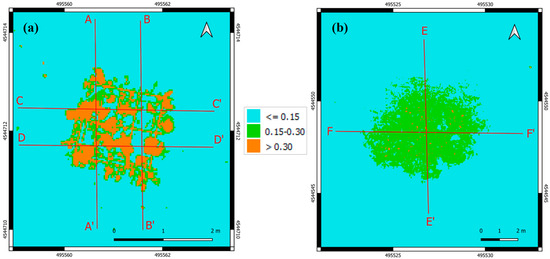
Figure 13.
HPI orthomosaic image excerpted over the plastic target (a) and the natural target (b).
The plastic target calls for high HPI values (>0.30), distributed in a patchy but coherent pattern across the structure. This reflects the wide spectral spread between Green/Red and Red Edge responses that is typical of heterogeneous plastics.
In contrast, the natural target (Figure 13b) shows a much more compact distribution, with most values falling in the intermediate range (0.15–0.30) and only sparse outliers reaching the highest class. The water, as expected, consistently belongs to the lowest class (≤0.15), confirming its uniform spectral response across the considered bands.
The quantitative analysis carried out through the transects confirms the visual inspection; see Figure 14 and Figure 15.
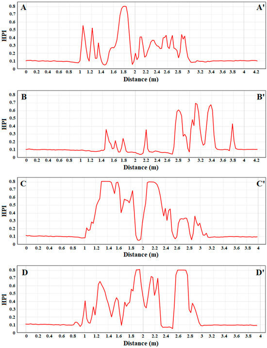
Figure 14.
HPI evaluated along the transects (A–A′, B–B′, C–C′, D–D′) traced on the plastic target. The x-axis represents the distance in meters along each profile, and the y-axis shows the values of the HPI.
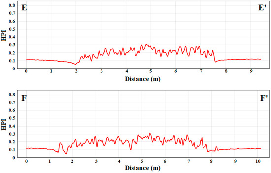
Figure 15.
HPI evaluated along the two transects (E–E′, F–F′) traced on the natural target. The x-axis represents the distance in meters along each profile, and the y-axis shows the values of the HPI.
Over the plastic target, see Figure 14, HPI values frequently exceed 0.7, with sharp oscillations and pronounced peaks corresponding to different plastic items. This irregular pattern mirrors the heterogeneity of the target, with abrupt changes along very short distances.
By contrast, over the natural target, see Figure 15, HPI values remain flat and stable, generally between 0.1 and 0.3. Minor fluctuations are present but never reach the high values typical of plastics, confirming the homogeneity of vegetation mats compared to synthetic materials.
The ranges of PDI and HPI for water, vegetation, and plastics are summarized in Table 4.
Table 4.
Range of PDI and HPI values evaluated within the plastic target, natural target, and surrounding water.
Both indices demonstrate good performance when distinguishing plastics from water, as the latter consistently remains in the lowest classes. However, the HPI demonstrates a wider dynamic range and greater robustness when discriminating plastics from the natural target, thanks to its explicit incorporation of variability. In practice, this means that PDI is more effective for highlighting plastics against aquatic backgrounds, while HPI is more suitable for separating plastics from spectrally similar natural materials.
Together, the two indices offer complementary perspectives: PDI captures the strong visible reflectance of plastics, whereas HPI formalizes their inherent heterogeneity. The combined use of these indices therefore enhances the reliability of UAV-based multispectral monitoring, providing a robust methodological framework for detecting plastics under complex freshwater conditions.
To provide an objective validation of the proposed indices, a quantitative classification analysis was performed using manually labeled training regions corresponding to plastics, floating vegetation, and water. Confusion matrices were generated to compute standard classification metrics, including Overall Accuracy, Kappa coefficient, and F1-scores for each class.
The results, summarized in Table 5, confirm the robustness of the proposed indices. The PDI achieved an Overall Accuracy of 89% and Kappa of 0.83, effectively distinguishing plastics from water. The HPI obtained an Overall Accuracy of 86% and Kappa of 0.78, performing best in separating plastics from vegetation. When both indices were combined, the F1-score for the plastic class reached 0.91, indicating strong complementarity between the two indices.
Table 5.
Quantitative validation results for PDI and HPI indices.
3.4. Thermal Results
The orthomosaic obtained using thermal measurements is depicted in Figure 16 for the plastic (a) and natural (b) target.
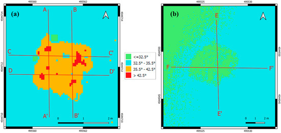
Figure 16.
Thermal orthomosaic image of the plastic target (a) and the natural target (b), showing temperatures in degrees Celsius (°C).
The signature of the plastic target (panel (a)) reveals a heterogeneous distribution of surface temperatures, with the warmer zones, highlighted in red, resulting in a larger thermal emissivity or direct exposure to radiation, whereas cooler areas, shown in cyan, are associated with water-covered surfaces or shaded portions of the target.
In contrast, panel (b) displays the natural target, composed of floating vegetation and organic debris. Here, the thermal pattern is noticeably cooler than the previous one and more homogeneous, exhibiting fewer sharp temperature gradients and a more continuous thermal response across the surface. Four classes were defined using empirical thresholds to highlight differences between water, vegetation, and plastic.
The differences observed in Figure 16 can be directly related to the intrinsic physical and material properties of the targets. Plastic materials often display complex geometries and variable reflectivity, color and composition, which collectively lead to localized variations in heat absorption and emission. Specific components, such as graphite polystyrene elements, can act as localized thermal hotspots, generating sharp peaks in temperature. On the other hand, natural floating vegetation is more uniform in structure and moisture content, leading to efficient heat dissipation and a stable thermal footprint that closely matches the surrounding water temperature.
The quantitative analysis, depicted in Figure 17 and Figure 18, refers to the evaluation of the thermal radiation over transects selected within the plastic and natural target, respectively. In Figure 17, the thermal profiles are depicted along transects A–A′, B–B′, C–C′, and D–D′, related to the plastic target.
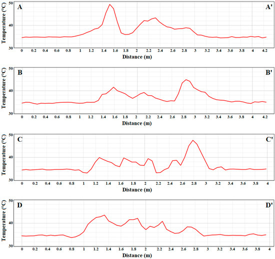
Figure 17.
Thermal response evaluated along with the transects (A–A′, B–B′, C–C′, D–D′) for the plastic target. The x-axis represents the distance in meters along each profile, while the y-axis indicates the temperature values, expressed in °C.
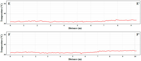
Figure 18.
Thermal response evaluated along with the transects E–E′ e F–F′ for the natural target. The x-axis represents the distance in meters along each profile, while the y-axis indicates the temperature values, expressed in °C.
It can be noted that the aquatic environment has a quite stable temperature of around 34 °C. The thermal behavior of the plastic target is more irregular, with sharp temperature peaks reaching up to 49 °C. These fluctuations mirror the heterogeneous nature of the plastic target: different shapes, colors, and material types absorb and emit heat differently. In particular, regions containing graphite polystyrene elements (marked as component 4 in Figure 1) stand out as pronounced hotspots, producing clearly recognizable peaks in the thermal curves. Overall, the profiles convey a vivid picture of the plastic target as a patchwork of thermally distinct zones, each reacting differently to the surrounding environment.
In contrast, Figure 18 shows the thermal profiles along transects E–E′ and F–F′ for the natural target.
Here, the curves are smooth and continuous, with only minor temperature variations. The floating leaves and organic debris display a uniform thermal response, closely matching the surrounding water temperature. Unlike the plastic target, no localized hotspots appear, highlighting the efficient heat distribution within natural materials. This steady thermal behavior reflects the homogeneous composition and moisture-rich structure of the vegetation, which helps maintain a balanced heat flow and minimizes abrupt temperature differences.
4. Discussion
The Lake Calore experiment, conducted within the framework of the ECOMARE project, offered a unique opportunity to evaluate UAV-based multisensor systems’ ability to monitor plastic debris over inland waters. The deployment of three UAV platforms equipped with optical, multispectral, and thermal sensors allowed for the investigation of floating plastics from complementary perspectives, demonstrating that the benefit of such an approach lies not in a single dataset but in their synergistic integration. This perspective reflects a broader trend in environmental remote sensing, where the fusion of heterogeneous information streams is increasingly recognized as essential for tackling complex monitoring challenges.
Although the single-field campaign provided controlled conditions, this may limit the transferability of the results to more complex environments. Real-world factors such as water turbidity, surface roughness, and varying solar illumination can modify spectral contrast and influence index-based discrimination, which must be taken into account for the scalability of the approach. For example, higher turbidity or rougher surfaces can reduce the reflectance difference between plastics and water, while low solar angles may alter apparent brightness and increase shadowing effects.
It should be noted that the study was conducted in a single lake at a single time point, which limits the generalization of the results. Future research should validate the proposed indices and multisensor approach under different seasons, water conditions, and illumination scenarios to fully assess robustness and applicability.
Moreover, the relatively low signal-to-noise ratio of the Mavic 3’s NIR band may constrain reproducibility across sensors. Future applications should therefore include multi-temporal acquisitions under different illumination and water conditions, and tests with radiometrically calibrated or higher dynamic range sensors should be carried out to improve scalability and cross-platform consistency.
From a spectral viewpoint, the findings indicate that the Green and Red bands provided the most robust and reliable separation between the plastics and their surrounding environment. Although several studies have reported that plastic generally exhibits strong reflectance in the NIR region, the presence of water on or around the target significantly reduces the measured signal. This behavior can be explained by a combination of factors, including wet-plastic effects, water absorption, sensor limitations, and illumination geometry. These findings underscore the importance of context-specific calibration and methodological adaptation when applying spectral approaches to plastic detection in inland waters, as the direct transfer of algorithms validated in terrestrial or coastal settings may lead to reduced accuracy.
The stronger performance of the Green and Red bands compared to the NIR can be explained by both physical and sensor-related factors. Water strongly absorbs near-infrared radiation around 840 nm, reducing reflectance from wet or partially submerged plastics, while the Mavic 3’s NIR channel exhibits a lower signal-to-noise ratio. In contrast, the visible bands remain more responsive to differences in color, surface texture, and illumination geometry, providing higher contrast between plastics and water.
The heterogeneity of the plastic assemblage proved to be another diagnostic feature. Comprising bottles, containers, and different types of polystyrene, the artificial target produced highly variable reflectance signatures, with sharp oscillations in the visible bands. This contrasted with the homogeneous behavior of the natural vegetation mat, which returned smooth and stable profiles across all spectral domains. The introduction of the HPI formalized this difference, capturing variability as a diagnostic marker of synthetic debris. Together with the PDI, which emphasized absolute reflectance contrasts, these indices demonstrated the potential of UAV-based multispectral analysis to not only detect plastics but also to characterize their internal diversity, paving the way for automatic classification workflows.
The statistical analysis presented in Section 3.3 quantitatively confirms the enhanced discriminative performance of PDI and HPI, supporting the novelty and complementary nature of these indices for UAV-based plastic detection.
The quantitative validation presented in Table 5 further confirms the reliability of the proposed indices. Both PDI and HPI achieved high accuracy values and showed complementary behavior, demonstrating that their combined use enhances the discrimination of plastics from natural materials and water. This consistency between spectral interpretation and statistical validation reinforces the robustness of the proposed approach.
The achieved accuracy metrics (Overall Accuracy > 0.85, Kappa > 0.78) confirm the robustness of both indices, while their combined application (OA = 0.92, Kappa = 0.86) demonstrates their complementarity and operational reliability under real field conditions. Thermal sensing added a further dimension to the analysis. Plastics exhibited localized hotspots with temperature differences exceeding 15°C compared to surrounding water, a reflection of their variable emissivity, geometry, and exposure conditions. The natural vegetation, on the other hand, displayed near-isothermal behavior, closely aligned with water temperature. These findings support the idea that thermal data are not merely complementary but are, in some cases, indispensable, particularly in scenarios where optical or multispectral acquisitions may be compromised by low illumination, cloud cover, or other atmospheric factors.
Thermal contrasts between vegetation and plastics arise from differences in emissivity and moisture content. Wet vegetation has high emissivity and retains water, which stabilizes its temperature, while dry plastics heat and cool rapidly due to their lower moisture content. These differences enhance the temperature contrast observed in thermal imagery, aiding in the detection of plastics against vegetated backgrounds.
It should be noted that thermal contrast between plastics and water may decrease in colder seasons, potentially reducing the effectiveness of thermal data. Future studies should include multi-seasonal acquisitions to assess performance under varying temperature conditions.
Equally important were the operational aspects of the campaign. The use of RTK positioning ensured centimetric accuracy, while systematic flight planning and rigorous photogrammetric processing guaranteed the coherence of the multisensor datasets. Such methodological rigor is crucial when the objective is not only presence/absence detection but also the detailed assessment of the material composition, spatial distribution, and temporal variability of plastic debris.
Overall, this study reinforces the notion that UAV-based multisensor monitoring represents a paradigm shift in the observation of plastic pollution: moving away from reliance on “canonical” spectral bands or single-sensor approaches toward a more flexible, context-sensitive, and integrated strategy.
5. Conclusions
The results of this work highlight the key role that UAV-based multisensor platforms can play in the monitoring of plastic debris in freshwater systems. By combining high-resolution optical, multispectral, and thermal imagery, it was possible not only to detect plastics with a high degree of confidence but also to characterize their heterogeneity and distinguish them from natural organic matter. This multidimensional capability is particularly relevant given the inherently diverse nature of anthropogenic debris and its tendency to blend with natural materials.
A key conclusion concerns the spectral response of plastics in aquatic environments. When imaging a heterogeneous plastic target partially submerged in lake water using the DJI Mavic 3 Multispectral, higher reflectance values were observed in the Green (560 nm) and Red (650 nm) bands compared to the Red Edge (730 nm) and Near-Infrared (860 ± 26 nm) bands. The reduced plastic-water contrast in the NIR is primarily caused by the strong absorption of radiation by water near 840 nm, which significantly attenuates the signals reflected from partially wet or partially submerged plastics. Controlled laboratory studies have shown that a thin film of water on a plastic surface decreases the diffuse component of reflected light, effectively masking the typical reflectance of dry material. Consequently, when plastics are wet or slightly submerged, their NIR reflectance is further reduced.
This behavior results from the combined influence of water absorption, sensor sensitivity, and illumination geometry. The limited sensitivity and lower signal-to-noise ratio of the Mavic 3’s NIR sensor, together with the inherent attenuation of NIR radiation in water, further reduce the recorded signal, whereas the visible bands remain more stable and luminous. Additionally, since the survey was conducted near solar noon, the high solar elevation enhanced specular reflection (sun-glint) from the water surface, increasing apparent brightness in the visible bands and further reducing the diffuse NIR contribution.
Overall, these findings demonstrate that visible bands, particularly Green and Red, can outperform NIR in plastic detection in inland water environments, emphasizing the importance of considering surface wetness, sensor characteristics, and illumination conditions when interpreting multispectral UAV imagery.
The development of two novel indices, the PDI and the HPI, represents an additional step toward operational monitoring. By enhancing contrasts with water and quantifying intra-target variability, these indices provide a methodological basis for scaling UAV-based observations to broader monitoring frameworks. They also hold significant promise for integration into machine learning pipelines, enabling the automated, real-time classification of floating plastics.
Beyond the technical findings, the study demonstrates that the effectiveness of UAV-based monitoring depends on methodological rigor. Flight planning, RTK-based positioning, and standardized photogrammetric workflows are not ancillary details but core components of a successful monitoring strategy. The Lake Calore campaign illustrates how such rigor enables the construction of coherent, multi-domain datasets that can reliably inform scientific research and environmental policy.
In the future, the methodological framework validated in this study could be extended to a variety of aquatic settings, from rivers to coastal waters. Its scalability makes it a promising candidate for integration into national or regional monitoring programs, where cost-effective, high-resolution, and flexible tools are urgently needed to address the global challenge of plastic pollution. By exploiting the complementarity of optical, multispectral, and thermal sensors, UAVs can contribute to the development of next-generation monitoring systems, bridging the gap between localized field campaigns and large-scale satellite-based observations.
Author Contributions
Conceptualization, N.A.F.; methodology, N.A.F., A.V. (Anna Verlanti) and L.D.R.; software, N.A.F., A.V. (Anna Verlanti) and L.D.R.; validation, ALL; data curation, N.A.F., A.V. (Anna Verlanti) and L.D.R.; writing—original draft preparation, ALL; writing—review and editing, ALL; visualization, N.A.F., A.V. (Anna Verlanti) and L.D.R. All authors have read and agreed to the published version of the manuscript.
Funding
These activities are partially funded by the European Union—Next Generation EU and the Italian Ministry of University and Research (MUR) under the Research Projects of National Relevance (PRIN) program “multi-layEr approaCh to detect and analyze cOastal aggregation of MAcRo-plastic littEr (ECOMARE)”, project ID 2022C3X37E.
Data Availability Statement
The original contributions presented in this study are included in the article. Further inquiries can be directed to the corresponding author.
Acknowledgments
The authors gratefully acknowledge the Consorzio di Bonifica dell’Ufita for its valuable collaboration and support in authorizing and facilitating the field operations at Lake Calore. The agreement established with the Consortium was essential to ensure the safe and compliant execution of the experimental campaign within the regulatory framework governing Italian inland waters. The authors also wish to thank the Consortium’s technical staff for their logistical assistance during the UAV survey activities.
Conflicts of Interest
The authors declare no conflicts of interest.
References
- Thiagarajan, C.; Devarajan, Y. The Urgent Challenge of Ocean Pollution: Impacts on Marine Biodiversity and Human Health. Reg. Stud. Mar. Sci. 2025, 81, 103995. [Google Scholar] [CrossRef]
- Simon, N.; Schulte, M.L. Stopping Global Plastic Pollution: The Case for an International Convention, 1st ed.; Ecology/Heinrich Böll Foundation: Berlin, Germany, 2017; ISBN 978-3-86928-159-9. [Google Scholar]
- Gall, S.C.; Thompson, R.C. The Impact of Debris on Marine Life. Mar. Pollut. Bull. 2015, 92, 170–179. [Google Scholar] [CrossRef]
- Beaumont, N.J.; Aanesen, M.; Austen, M.C.; Börger, T.; Clark, J.R.; Cole, M.; Hooper, T.; Lindeque, P.K.; Pascoe, C.; Wyles, K.J. Global Ecological, Social and Economic Impacts of Marine Plastic. Mar. Pollut. Bull. 2019, 142, 189–195. [Google Scholar] [CrossRef]
- Lau, W.W.Y.; Shiran, Y.; Bailey, R.M.; Cook, E.; Stuchtey, M.R.; Koskella, J.; Velis, C.A.; Godfrey, L.; Boucher, J.; Murphy, M.B.; et al. Evaluating Scenarios toward Zero Plastic Pollution. Science 2020, 369, 1455–1461. [Google Scholar] [CrossRef]
- Li, W.C.; Tse, H.F.; Fok, L. Plastic Waste in the Marine Environment: A Review of Sources, Occurrence and Effects. Sci. Total Environ. 2016, 566–567, 333–349. [Google Scholar] [CrossRef] [PubMed]
- Oluniyi Solomon, O.; Palanisami, T. Microplastics in the Marine Environment: Current Status, Assessment Methodologies, Impacts and Solutions. J. Pollut. Eff. Cont. 2016, 4, 1000161. [Google Scholar] [CrossRef]
- Sheppard, C.R.C. World Seas: An Environmental Evaluation, 2nd ed.; Academic Press, an Imprint of Elsevier: London, UK, 2019; ISBN 978-0-12-805204-4. [Google Scholar]
- Toussaint, B.; Raffael, B.; Angers-Loustau, A.; Gilliland, D.; Kestens, V.; Petrillo, M.; Rio-Echevarria, I.M.; Van Den Eede, G. Review of Micro- and Nanoplastic Contamination in the Food Chain. Food Addit. Contam. Part A 2019, 36, 639–673. [Google Scholar] [CrossRef]
- Prata, J.C.; Da Costa, J.P.; Lopes, I.; Duarte, A.C.; Rocha-Santos, T. Environmental Exposure to Microplastics: An Overview on Possible Human Health Effects. Sci. Total Environ. 2020, 702, 134455. [Google Scholar] [CrossRef]
- Rhodes, C.J. Solving the Plastic Problem: From Cradle to Grave, to Reincarnation. Sci. Prog. 2019, 102, 218–248. [Google Scholar] [CrossRef]
- Gallo, F.; Fossi, C.; Weber, R.; Santillo, D.; Sousa, J.; Ingram, I.; Nadal, A.; Romano, D. Marine Litter Plastics and Microplastics and Their Toxic Chemicals Components: The Need for Urgent Preventive Measures. Environ. Sci. Eur. 2018, 30, 13. [Google Scholar] [CrossRef] [PubMed]
- Salgado-Hernanz, P.M.; Bauzà, J.; Alomar, C.; Compa, M.; Romero, L.; Deudero, S. Assessment of Marine Litter through Remote Sensing: Recent Approaches and Future Goals. Mar. Pollut. Bull. 2021, 168, 112347. [Google Scholar] [CrossRef] [PubMed]
- Themistocleous, K.; Papoutsa, C.; Michaelides, S.; Hadjimitsis, D. Investigating Detection of Floating Plastic Litter from Space Using Sentinel-2 Imagery. Remote Sens. 2020, 12, 2648. [Google Scholar] [CrossRef]
- Topouzelis, K.; Papageorgiou, D.; Suaria, G.; Aliani, S. Floating Marine Litter Detection Algorithms and Techniques Using Optical Remote Sensing Data: A Review. Mar. Pollut. Bull. 2021, 170, 112675. [Google Scholar] [CrossRef]
- Duarte, M.M.; Azevedo, L. Erratum to “Automatic Detection and Identification of Floating Marine Debris Using Multispectral Satellite Imagery”. IEEE Trans. Geosci. Remote Sens. 2023, 61, 2002315. [Google Scholar] [CrossRef]
- Basu, B.; Sannigrahi, S.; Sarkar Basu, A.; Pilla, F. Development of Novel Classification Algorithms for Detection of Floating Plastic Debris in Coastal Waterbodies Using Multispectral Sentinel-2 Remote Sensing Imagery. Remote Sens. 2021, 13, 1598. [Google Scholar] [CrossRef]
- De Giglio, M.; Dubbini, M.; Cortesi, I.; Maraviglia, M.; Parisi, E.I.; Tucci, G. Plastics Waste Identification in River Ecosystems by Multispectral Proximal Sensing: A Preliminary Methodology Study. Water Environ. J. 2021, 35, 569–579. [Google Scholar] [CrossRef]
- Vidal, M.; Gowen, A.; Amigo, J.M. NIR Hyperspectral Imaging for Plastics Classification. NIR News 2012, 23, 13–15. [Google Scholar] [CrossRef]
- Kremezi, M.; Kristollari, V.; Karathanassi, V.; Topouzelis, K.; Kolokoussis, P.; Taggio, N.; Aiello, A.; Ceriola, G.; Barbone, E.; Corradi, P. Pansharpening PRISMA Data for Marine Plastic Litter Detection Using Plastic Indexes. IEEE Access 2021, 9, 61955–61971. [Google Scholar] [CrossRef]
- Tasseron, P.; Van Emmerik, T.; Peller, J.; Schreyers, L.; Biermann, L. Advancing Floating Macroplastic Detection from Space Using Experimental Hyperspectral Imagery. Remote Sens. 2021, 13, 2335. [Google Scholar] [CrossRef]
- Goddijn-Murphy, L.; Williamson, B.J.; McIlvenny, J.; Corradi, P. Using a UAV Thermal Infrared Camera for Monitoring Floating Marine Plastic Litter. Remote Sens. 2022, 14, 3179. [Google Scholar] [CrossRef]
- Garaba, S.P.; Acuña-Ruz, T.; Mattar, C.B. Hyperspectral Longwave Infrared Reflectance Spectra of Naturally Dried Algae, Anthropogenic Plastics, Sands and Shells. Earth Syst. Sci. Data 2020, 12, 2665–2678. [Google Scholar] [CrossRef]
- Palombi, L.; Raimondi, V. Experimental Tests for Fluorescence LIDAR Remote Sensing of Submerged Plastic Marine Litter. Remote Sens. 2022, 14, 5914. [Google Scholar] [CrossRef]
- Spizzichino, V.; Caneve, L.; Colao, F.; Ruggiero, L. Characterization and Discrimination of Plastic Materials Using Laser-Induced Fluorescence. Appl. Spectrosc. 2016, 70, 1001–1008. [Google Scholar] [CrossRef] [PubMed]
- Piruska, A.; Nikcevic, I.; Lee, S.H.; Ahn, C.; Heineman, W.R.; Limbach, P.A.; Seliskar, C.J. The Autofluorescence of Plastic Materials and Chips Measured under Laser Irradiation. Lab Chip 2005, 5, 1348. [Google Scholar] [CrossRef] [PubMed]
- Kalogirou, E.; Christofi, K.; Makri, D.; Iqbal, M.A.; La Pegna, V.; Tzouvaras, M.; Mettas, C.; Hadjimitsis, D. Oil Spill Detection Using Convolutional Neural Networks and Sentinel-1 SAR Imagery. Int. Arch. Photogramm. Remote Sens. Spatial Inf. Sci. 2025, 48, 757–764. [Google Scholar] [CrossRef]
- Meng, T.; Nunziata, F.; Yang, X.; Buono, A.; Chen, K.-S.; Migliaccio, M. Scattering Model-Based Oil-Slick-Related Parameters Estimation from Radar Remote Sensing: Feasibility and Simulation Results. IEEE Trans. Geosci. Remote Sens. 2024, 62, 4203412. [Google Scholar] [CrossRef]
- Jamal, S.; Sun, G.; Li, Y.; Khan, A.Q.; Zhang, Y.; Verlanti, A.; Nunziata, F. CWCM-Net: A Novel Feature Fusion Method for Oil Spill Detection Using Single- and Quad-Polarization SAR Data. IEEE J. Sel. Top. Appl. Earth Obs. Remote Sens. 2025, 18, 19115–19128. [Google Scholar] [CrossRef]
- Savastano, S.; Cester, I.; Perpinya, M.; Romero, L. A First Approach to the Automatic Detection of Marine Litter in SAR Images Using Artificial Intelligence. In Proceedings of the 2021 IEEE International Geoscience and Remote Sensing Symposium IGARSS, Brussels, Belgium, 11–16 July 2021; IEEE: Brussels, Belgium, 2021; pp. 8704–8707. [Google Scholar]
- Davaasuren, N.; Marino, A.; Boardman, C.; Alparone, M.; Nunziata, F.; Ackermann, N.; Hajnsek, I. Detecting Microplastics Pollution in World Oceans Using Sar Remote Sensing. In Proceedings of the IGARSS 2018—2018 IEEE International Geoscience and Remote Sensing Symposium, Valencia, Spain, 22–27 July 2018; IEEE: Valencia, Spain, 2018; pp. 938–941. [Google Scholar]
- Simpson, M.D.; Marino, A.; De Maagt, P.; Gandini, E.; Hunter, P.; Spyrakos, E.; Tyler, A.; Telfer, T. Monitoring of Plastic Islands in River Environment Using Sentinel-1 SAR Data. Remote Sens. 2022, 14, 4473. [Google Scholar] [CrossRef]
- Chen, Z.; Li, F. Mapping Plastic-Mulched Farmland with C-Band Full Polarization SAR Remote Sensing Data. Remote Sens. 2017, 9, 1264. [Google Scholar] [CrossRef]
- Da Costa, T.S.; Felício, J.M.; Matos, S.A.; Costa, J.R.; Fernandes, C.A.; Fonseca, N.J.G. Monitoring Plastic Accumulations in a River Environment Using Machine Learning on Sentinel-1 SAR Data. In Proceedings of the 2025 19th European Conference on Antennas and Propagation (EuCAP), Stockholm, Sweden, 30 March–4 April 2025; IEEE: Stockholm, Sweden, 2025; pp. 1–5. [Google Scholar]
- Garaba, S.P.; Aitken, J.; Slat, B.; Dierssen, H.M.; Lebreton, L.; Zielinski, O.; Reisser, J. Sensing Ocean Plastics with an Airborne Hyperspectral Shortwave Infrared Imager. Environ. Sci. Technol. 2018, 52, 11699–11707. [Google Scholar] [CrossRef]
- Jakovljevic, G.; Govedarica, M.; Alvarez-Taboada, F. A Deep Learning Model for Automatic Plastic Mapping Using Unmanned Aerial Vehicle (UAV) Data. Remote Sens. 2020, 12, 1515. [Google Scholar] [CrossRef]
- Maharjan, N.; Miyazaki, H.; Pati, B.M.; Dailey, M.N.; Shrestha, S.; Nakamura, T. Detection of River Plastic Using UAV Sensor Data and Deep Learning. Remote Sens. 2022, 14, 3049. [Google Scholar] [CrossRef]
- Taddia, Y.; Corbau, C.; Buoninsegni, J.; Simeoni, U.; Pellegrinelli, A. UAV Approach for Detecting Plastic Marine Debris on the Beach: A Case Study in the Po River Delta (Italy). Drones 2021, 5, 140. [Google Scholar] [CrossRef]
- Geraeds, M.; Van Emmerik, T.; De Vries, R.; Bin Ab Razak, M.S. Riverine Plastic Litter Monitoring Using Unmanned Aerial Vehicles (UAVs). Remote Sens. 2019, 11, 2045. [Google Scholar] [CrossRef]
- Denih, A.; Matsumoto, T.; Rachman, I.; Putra, G.R.; Anggraeni, I.; Kurnia, E.; Suhendar, E.; Simamora, A.M. Identification of Plastic Waste with Unmanned Aerial Vehicle (UAV) Using Deep Learning and Internet of Things (IoT). J. Hazard. Mater. Adv. 2025, 18, 100622. [Google Scholar] [CrossRef]
- Zhou, S.; Kaufmann, H.; Bohn, N.; Bochow, M.; Kuester, T.; Segl, K. Identifying Distinct Plastics in Hyperspectral Experimental Lab-, Aircraft-, and Satellite Data Using Machine/Deep Learning Methods Trained with Synthetically Mixed Spectral Data. Remote Sens. Environ. 2022, 281, 113263. [Google Scholar] [CrossRef]
- Topouzelis, K.; Papakonstantinou, A.; Garaba, S.P. Detection of Floating Plastics from Satellite and Unmanned Aerial Systems (Plastic Litter Project 2018). Int. J. Appl. Earth Obs. Geoinf. 2019, 79, 175–183. [Google Scholar] [CrossRef]
- Goddijn-Murphy, L.; Martínez-Vicente, V.; Dierssen, H.M.; Raimondi, V.; Gandini, E.; Foster, R.; Chirayath, V. Emerging Technologies for Remote Sensing of Floating and Submerged Plastic Litter. Remote Sens. 2024, 16, 1770. [Google Scholar] [CrossRef]
- Rettig, R.; Becker, F.; Berghoff, A.; Binkele, T.; Butter, W.M.; Floehr, T.; Kumm, M.; Leluschko, C.; Littau, F.; Reinders, E.; et al. Multi-Resolution Remote Sensing Dataset for the Detection of Anthropogenic Litter: A Multi-Platform and Multi-Sensor Approach. Data 2025, 10, 113. [Google Scholar] [CrossRef]
- Nunziata, F.; Serafino, F.; Vicari, A.; Migliaccio, M.; Bianco, A.; Verlanti, A.; Di Michele, L.; Cotroneo, Y.; Aulicino, G.; Famiglietti, N.A.; et al. Multi-Layer Approach to Detect and Analyze Coastal Aggregation of Macro-Plastic Litter. In Proceedings of the 2024 IEEE International Workshop on Metrology for the Sea; Learning to Measure Sea Health Parameters (MetroSea), Portorose, Slovenia, 14–16 October 2024; IEEE: Portorose, Slovenia, 2024; pp. 364–368. [Google Scholar]
- Simpson, M.D.; Marino, A.; De Maagt, P.; Gandini, E.; De Fockert, A.; Hunter, P.; Spyrakos, E.; Telfer, T.; Tyler, A. Investigating the Backscatter of Marine Plastic Litter Using a C- and X-Band Ground Radar, during a Measurement Campaign in Deltares. Remote Sens. 2023, 15, 1654. [Google Scholar] [CrossRef]
- Felício, J.M.; Costa, T.S.; Vala, M.; Leonor, N.; Costa, J.R.; Marques, P.; Moreira, A.A.; Caldeirinha, R.F.S.; Matos, S.A.; Fernandes, C.A.; et al. Feasibility of Radar-Based Detection of Floating Macroplastics at Microwave Frequencies. IEEE Trans. Antennas Propagat. 2024, 72, 2766–2779. [Google Scholar] [CrossRef]
- Alboody, A.; Vandenbroucke, N.; Porebski, A.; Sawan, R.; Viudes, F.; Doyen, P.; Amara, R. A New Remote Hyperspectral Imaging System Embedded on an Unmanned Aquatic Drone for the Detection and Identification of Floating Plastic Litter Using Machine Learning. Remote Sens. 2023, 15, 3455. [Google Scholar] [CrossRef]
- Moshtaghi, M.; Knaeps, E.; Sterckx, S.; Garaba, S.; Meire, D. Spectral Reflectance of Marine Macroplastics in the VNIR and SWIR Measured in a Controlled Environment. Sci. Rep. 2021, 11, 5436. [Google Scholar] [CrossRef] [PubMed]
- Biermann, L.; Clewley, D.; Martinez-Vicente, V.; Topouzelis, K. Finding Plastic Patches in Coastal Waters Using Optical Satellite Data. Sci. Rep. 2020, 10, 5364. [Google Scholar] [CrossRef] [PubMed]
- Guo, X.; Li, P. Mapping Plastic Materials in an Urban Area: Development of the Normalized Difference Plastic Index Using WorldView-3 Superspectral Data. ISPRS J. Photogramm. Remote Sens. 2020, 169, 214–226. [Google Scholar] [CrossRef]
- Guffogg, J.; Soto-Berelov, M.; Bellman, C.; Jones, S.; Skidmore, A. Beached Plastic Debris Index; a Modern Index for Detecting Plastics on Beaches. Mar. Pollut. Bull. 2024, 209, 117124. [Google Scholar] [CrossRef]
- Nunziata, F.; Famiglietti, N.A.; Vicari, A.; Memmolo, A.; Migliazza, R.; Verlanti, A.; Buono, A.; Migliaccio, M. An Experimental Campaign to Observe Floating Plastic Using a Multi-Sensor Strategy. In Proceedings of the OCEANS 2025 Brest, Brest, France, 16–19 June 2025; IEEE: Brest, France, 2025; pp. 1–4. [Google Scholar]
- INGV RING Working Group. Rete Integrata Nazionale GPS (RING); [Data set]; Istituto Nazionale di Geofisica e Vulcanologia (INGV): Roma, Italy, 2016. [Google Scholar] [CrossRef]
- Famiglietti, N.A.; Cecere, G.; Grasso, C.; Memmolo, A.; Vicari, A. A Test on the Potential of a Low Cost Unmanned Aerial Vehicle RTK/PPK Solution for Precision Positioning. Sensors 2021, 21, 3882. [Google Scholar] [CrossRef]
- Hu, C. Remote Detection of Marine Debris Using Satellite Observations in the Visible and near Infrared Spectral Range: Challenges and Potentials. Remote Sens. Environ. 2021, 259, 112414. [Google Scholar] [CrossRef]
- Holt, Z.K.; Khan, S.D.; Rodrigues, D.F. Hyperspectral Remote Sensing as an Environmental Plastic Pollution Detection Approach to Determine Occurrence of Microplastics in Diverse Environments. Environ. Pollut. 2025, 377, 126426. [Google Scholar] [CrossRef] [PubMed]
- Corbari, L.; Capodici, F.; Ciraolo, G.; Topouzelis, K. Marine Plastic Detection Using PRISMA Hyperspectral Satellite Imagery in a Controlled Environment. Int. J. Remote Sens. 2023, 44, 6845–6859. [Google Scholar] [CrossRef]
- Deng, R.; He, Y.; Qin, Y.; Chen, Q.; Chen, L. Measuring Pure Water Absorption Coefficient in the Near-Infrared Spectrum (900–2500 Nm). Natl. Remote Sens. Bull. 2012, 16, 192–206. [Google Scholar] [CrossRef]
- Bi, S.; Li, Y.; Wang, Q.; Lyu, H.; Liu, G.; Zheng, Z.; Du, C.; Mu, M.; Xu, J.; Lei, S.; et al. Inland Water Atmospheric Correction Based on Turbidity Classification Using OLCI and SLSTR Synergistic Observations. Remote Sens. 2018, 10, 1002. [Google Scholar] [CrossRef]
- Cui, M.; Sun, Y.; Huang, C.; Li, M. Water Turbidity Retrieval Based on UAV Hyperspectral Remote Sensing. Water 2022, 14, 128. [Google Scholar] [CrossRef]
- Röttgers, R.; McKee, D.; Utschig, C. Temperature and Salinity Correction Coefficients for Light Absorption by Water in the Visible to Infrared Spectral Region. Opt. Express 2014, 22, 25093–25108. [Google Scholar] [CrossRef]
- Wang, S.; Zhao, W.; Sun, D.; Li, Z.; Shen, C.; Bu, X.; Zhang, H. Unveiling Reflectance Spectral Characteristics of Floating Plastics across Varying Coverages: Insights and Retrieval Model. Opt. Express 2024, 32, 22078–22094. [Google Scholar] [CrossRef]
- Knaeps, E.; Sterckx, S.; Strackx, G.; Mijnendonckx, J.; Moshtaghi, M.; Garaba, S.P.; Meire, D. Hyperspectral-Reflectance Dataset of Dry, Wet and Submerged Marine Litter. Earth Syst. Sci. Data 2021, 13, 713–730. [Google Scholar] [CrossRef]
- Hedley, J.D.; Harborne, A.R.; Mumby, P.J. Technical Note: Simple and Robust Removal of Sun Glint for Mapping Shallow-water Benthos. Int. J. Remote Sens. 2005, 26, 2107–2112. [Google Scholar] [CrossRef]
- Stow, D.; Nichol, C.J.; Wade, T.; Assmann, J.J.; Simpson, G.; Helfter, C. Illumination Geometry and Flying Height Influence Surface Reflectance and NDVI Derived from Multispectral UAS Imagery. Drones 2019, 3, 55. [Google Scholar] [CrossRef]
- Kutser, T.; Vahtmäe, E.; Praks, J. A Sun Glint Correction Method for Hyperspectral Imagery Containing Areas with Non-Negligible Water Leaving NIR Signal. Remote Sens. Environ. 2009, 113, 2267–2274. [Google Scholar] [CrossRef]
- Sun, Y.; Qin, Q.; Ren, H.; Zhang, T.; Chen, S. Red-Edge Band Vegetation Indices for Leaf Area Index Estimation from Sentinel-2/MSI Imagery. IEEE Trans. Geosci. Remote Sens. 2020, 58, 826–840. [Google Scholar] [CrossRef]
- Widjaja Putra, B.T.; Soni, P. Evaluating NIR-Red and NIR-Red Edge External Filters with Digital Cameras for Assessing Vegetation Indices under Different Illumination. Infrared Phys. Technol. 2017, 81, 148–156. [Google Scholar] [CrossRef]
- Zeng, Y.; Hao, D.; Badgley, G.; Damm, A.; Rascher, U.; Ryu, Y.; Johnson, J.; Krieger, V.; Wu, S.; Qiu, H.; et al. Estimating Near-Infrared Reflectance of Vegetation from Hyperspectral Data. Remote Sens. Environ. 2021, 267, 112723. [Google Scholar] [CrossRef]
Disclaimer/Publisher’s Note: The statements, opinions and data contained in all publications are solely those of the individual author(s) and contributor(s) and not of MDPI and/or the editor(s). MDPI and/or the editor(s) disclaim responsibility for any injury to people or property resulting from any ideas, methods, instructions or products referred to in the content. |
© 2025 by the authors. Licensee MDPI, Basel, Switzerland. This article is an open access article distributed under the terms and conditions of the Creative Commons Attribution (CC BY) license (https://creativecommons.org/licenses/by/4.0/).