Article

Effectiveness of Unmanned Aerial Vehicle-Based LiDAR for Assessing the Impact of Catastrophic Windstorm Events on Timberland

1
College of Forestry, Wildlife and Environment, Auburn University, Auburn, AL 36849, USA
2
College of Agriculture, Health, and Natural Resources, Kentucky State University, Frankfort, KY 40601, USA
*
Author to whom correspondence should be addressed.
Drones 2025, 9(11), 756; https://doi.org/10.3390/drones9110756
Submission received: 27 August 2025 / Revised: 15 October 2025 / Accepted: 23 October 2025 / Published: 31 October 2025

Highlights

What are the main findings?
  • UAV—LiDAR combined with RGB imagery significantly improved mapping of wind-storm-damaged forests, achieving higher classification accuracy.
  • Random Forest classifier outperformed Maximum Likelihood and Decision Tree methods.
What are the implications of the main findings?
  • Incorporating LiDAR-derived canopy height models is crucial for accurate assess-ment of windstorm damage in forestland.
  • UAV—LiDAR integrated with UAV imagery enables efficient and scalable mapping for post-windstorm forest damage assessment and planning.

Abstract

The southeastern United States (US) is known for its highly productive forests, but they are under intense threat from increasing climate-induced windstorms like hurricanes and tornadoes. This study explored the effectiveness of unmanned aerial vehicles (UAVs) equipped with Light Detection and Ranging (LiDAR) to detect, classify, and map windstorm damage in ten pine-dominated forest stands (10–20 acres each). Three classification techniques, Random Forest (RF), Maximum Likelihood (ML), and Decision Tree (DT), were tested on two datasets: RGB imagery integrated with LiDAR-derived Canopy Height Model (CHM) and without LiDAR-CHM. Using LiDAR-CHM integrated datasets, RF achieved an average Overall Accuracy (OA) of 94.52% and a kappa coefficient (k) of 0.92, followed by ML (average OA = 89.52% and k = 0.85), and DT (average OA = 81.78% and k = 0.75). The results showed that RF consistently outperformed ML and DT in classification accuracy across all sites. Without LiDAR-CHM, the performance of all classifiers significantly declined, underscoring the importance of structural data in distinguishing among the classification categories (downed trees, standing trees, ground, and water). These findings highlight the role of UAV-derived LiDAR-CHM in improving classification accuracy for assessing the impact of windstorm damage on forest stands.

1. Introduction

The southeastern United States (US) is home to some of the world’s most productive forests, which contribute significantly to the country’s local and national economies. However, the escalating frequency of climate-induced disasters, particularly windstorm events, is adversely affecting the productivity, stability, and sustainability of forests within this region [1,2]. These extreme windstorm events snap and uproot trees, break branches, alter soil structure, and cause erosion, leading to loss of timber, decreased carbon sequestration, and destruction of habitat [3,4]. Additionally, they cause significant financial losses for landowners [3,5,6]. In 2018, Hurricane Michael caused significant damage to 958,387 hectares of forestland in Georgia, with a pre-hurricane value of approximately USD 762 million [7]. Hurricane Laura in 2020 had a timber loss valued at USD 1.2 billion [6]. Similarly, in Georgia, Hurricane Helene was estimated to have resulted in USD 1.28 billion in timber losses [8].
There is a short window for salvaging wind-damaged timber. Ref. [9] emphasized the importance of timely salvage operations for storm-damaged pine trees, recommending immediate harvesting for trees with severe damage to maximize resource recovery, while suggesting a 2–3-month window for uprooted trees to prevent decay from fungi and pests. Furthermore, storm-damaged forests are highly susceptible to secondary disturbances such as insect attacks, erosion, and wildfires [10], which can further diminish timber value and impede forest recovery. Therefore, early assessment of the nature, extent, and severity of damage is crucial, as it can help determine whether the stands are still viable and support salvage harvesting as needed. While on-the-ground field surveys have traditionally been used to estimate windstorm damage, they are expensive, labor-intensive, time-consuming, and pose a safety risk to the surveyors due to the snapped and leaning trees and the amount of debris on the ground [11,12]. Remote sensing technologies provide a rapid and detailed alternative, allowing for real-time data collection without having to traverse unsafe stands. When combined with automatic processing techniques, this technology enables precise details of large-scale areas and disturbances [13].
Various sensors and platforms can be utilized to gather remote sensing data. These sensors can be either passive, such as multispectral, hyperspectral, and thermal sensors, or active, such as Light Detection and Ranging (LiDAR) and Synthetic Aperture Radar (SAR). Similarly, various platforms are available, such as satellites, manned aircraft, and unmanned aerial vehicles (UAVs), which can be equipped with these sensors to obtain information at multiple scales [14,15]. Satellite or manned airborne systems may include high operational costs, safety risks, and limited temporal and spatial resolution [16,17,18,19]. UAVs can prove to be a valuable solution to address these limitations, given their low cost, high speed, flexibility in operating in diverse environments, and ability to capture highly precise information in all weather conditions [15,20,21]. UAVs, like other platforms, can support different sensors such as imaging sensors and LiDAR, enabling diverse forestry applications. Among these, LiDAR technology has emerged as one of the most capable tools for extensive research and quantifying the three-dimensional (3D) structure of forests [22,23,24].
LiDAR is an active remote sensing technology that utilizes a pulsed laser to precisely measure the Earth’s surface [14]. Given its ability to penetrate the canopy, provide within-canopy information, and accurately identify individual trees, LiDAR data are considered more advantageous and accurate than other methods [25,26,27]. Across platforms, it has been widely used to obtain estimates of tree height, tree density, forest composition, crown diameter, basal area, growing stock volume, leaf area index, and biomass [24,28,29,30,31]. UAV–LiDAR, in particular, benefits from low-altitude flights that can generate significantly greater return (or point) densities compared to manned airborne or satellite platforms [21,32,33,34], supporting precise measurement of individual trees and understory vegetation [35,36]. In practice, UAV–LiDAR has been used to identify and map vegetation [37], assess land-cover change [38], perform species identification [39], estimate individual tree dendrometric metrics [40], and support other forestry applications [41].
Complementing LiDAR, recent advancements in UAV technology have also enabled capturing centimeter-scale imagery with exceptional spatial and temporal resolution. This has allowed for detailed analysis of forest characteristics at a fine scale [20,42]. Ultrahigh-resolution UAV imagery (with spatial resolution in centimeters) incorporating complex surface details and textures provides an optimal platform for efficient vegetation studies, with proven efficiency at resolutions ranging from less than 2 cm to 7 cm [43,44,45,46,47]. Several studies have utilized high-resolution UAV imagery for windstorm damage assessment. Ref. [48] demonstrated the potential of high-resolution UAV imagery to recognize fallen trees using the Hough transformation algorithm, achieving a completeness of 75.7% and a correctness of 92.5%, indicating high reliability in detecting fallen logs. Ref. [49] developed an innovative method for automatically detecting dead or dying trees using UAV imagery. The results of their study indicated that dead trees could be identified using UAV imagery with a confidence level of over 80%. Prior studies have also utilized airborne LiDAR data [50,51,52] and terrestrial LiDAR data [53] to detect fallen trees and map woody debris. For instance, Ref. [52] suggested detecting fallen trees using airborne LiDAR data by combining short segments into complete stems with the Normalized Cut algorithm. This approach demonstrated the ability to identify about 90% of fallen stems while retaining over 80% accuracy. Similarly, Ref. [51] combined centimetric aerial imagery with airborne LiDAR data to detect standing dead trees and downed coarse woody debris, achieving high accuracy with 93.4% completeness and 94.5% correctness in the application area.
The effectiveness of UAV imagery and UAV–LiDAR largely depends on the type and quality of information that can be derived from them. Data collected from various remote sensing platforms, when integrated with diverse classification algorithms, help in extracting valuable ecological information [37,54,55]. This involves classifying each image pixel or cluster of pixels into different classes depending on their spectral, spatial, and temporal characteristics. The most widely used image classification techniques include parametric methods like Maximum Likelihood (ML) classification [42,56], non-parametric classification methods like traditional Decision Tree (DT) [57,58], and machine learning approaches such as Random Forest (RF) [51,59,60]. Other approaches, such as Support Vector Machines (SVM) and deep learning, have also been applied in similar studies [40,57,61]. Among these methods, researchers have gained substantial interest in machine learning classifiers given their ability to handle non-linear data effectively, offer higher classification accuracy, and provide user flexibility [37,62,63].
Integrating LiDAR data with imagery and applying various classification techniques has become increasingly popular for environmental monitoring, forest management, and disaster response [64,65,66,67]. For instance, Ref. [37] employed four classification algorithms (RF, Maximum Likelihood, Mahalanobis Distance, and Support Vector Machine) for mapping the vegetation of No Name Key, Florida. They used publicly available airborne LiDAR data and high-resolution NAIP imagery and conducted classification on two datasets: NAIP imagery only and NAIP combined with airborne LiDAR. Among the methods used, RF classification achieved the highest Overall Accuracy (OA) and kappa value (k) on the combined dataset (stacked image with NAIP imagery and LiDAR). While LiDAR primarily captures structural data, combining it with high-resolution imagery provides detailed spectral and textural data on crowns, canopy cover, and understory [68,69,70,71]. The integration of these datasets enhances the accuracy of tree height and canopy structure estimation, which is crucial for forestry applications like post-disaster damage assessments, timber volume estimation, species identification, and habitat modeling [11,39,64,66,72,73].
Although UAV imagery and UAV–LiDAR pose individual advantages, few studies have evaluated their integrated workflows for mapping and classifying windstorm-damaged forests. Given the increasing frequency and scale of windstorms like hurricanes and tornadoes in the southeastern US, there is a crucial need for rapid, more efficient, and fine-scale techniques to evaluate forest damage and inform sustainable post-disaster decision making. While some studies have employed airborne and terrestrial data sources to identify windstorm-downed trees [50,51,52], the use of UAV imagery and LiDAR data together for mapping windstorm disturbances has been relatively unexplored. With the increasing accessibility of high-resolution UAV sensors, there is significant potential to further investigate their combined effectiveness in accurately detecting and classifying extensive windstorm damage in forested areas.
In this study, we examined the effectiveness of UAV–LiDAR and UAV imagery in detecting, classifying, and mapping windstorm-damaged forest stands in the southeastern US. This study aimed to (1) determine whether adding LiDAR-derived Canopy Height Model (CHM) to RGB (with vegetation indices) improves classification of windstorm-impacted forest stands; (2) compare the performance of three classification algorithms, Random Forest (RF), Maximum Likelihood (ML), and Decision Tree (DT), in classifying windstorm damage using UAV-derived RGB imagery, with and without LiDAR-derived CHM; and (3) produce fine-scale damage maps for tornado and hurricane-damaged sites in Alabama, Georgia, and Florida. This study is crucial for assessing the damage caused by windstorms, aids in efficiently allocating resources for recovery efforts, and provides landowners, foresters, and stakeholders with detailed observations and information for fine-scale post-disaster planning and management.

2. Materials and Methods

2.1. Study Area

The study included ten sites (Figure 1) damaged by hurricanes and tornadoes in 2022 and 2023. Six of the ten sites were damaged by tornadoes in Alabama, two tornado sites in Georgia, and two hurricane sites in Florida. For the study, only a small portion of the damaged areas were sampled and were primarily based on forest stand characteristics (pine plantation) and landowner property boundaries (four sites were approximately 20 acres, and the remaining six were approximately 10 acres in area). Although some sites are inland, all sites are located in the southeastern US, where weather and extreme events are highly influenced by the Gulf of Mexico and the Atlantic Ocean, making them vulnerable to windstorm hazards [74]. The most common tree species found in all ten sites was loblolly pine (Pinus taeda), with only a few occurrences of hardwood species like Quercus spp. on some sites.
The National Weather Service (NWS) Damage Assessment Toolkit (DAT), which is a GIS-based system containing information on points, routes, track centerlines, and damage swaths of tornadoes and convective wind events, was used to identify tornado sites. Hurricane data were obtained from the National Oceanic and Atmospheric Administration’s (NOAA) National Hurricane Center (NHC). Based upon the preliminary damage path analysis from NWS DAT and NOAA NHC, the following counties were found to be severely affected by tornadoes and hurricanes: Tuscaloosa (Sites 1, 2, and 3), Tallapoosa (Site 5), Bibb (Site 6), and Coosa (Site 4) in Alabama; Troup (Sites 7 and 8) in Georgia; and Taylor (Sites 9 and 10) in Florida. Field visits were conducted to confirm the damage and finalize the study area.

2.2. Data Acquisition

2.2.1. Forest Inventory

Stand-level data were collected using fixed-radius 1/10th acre plots. On sites 11–20 acres, six plots were randomly selected per site, while on sites ≤10 acres, three plots were randomly selected per site [75,76]. Within each plot, tree measurements were recorded, which included tree count, tree species, diameter at breast height (dbh), diameter at both ends of fallen or uprooted trees, height of standing trees (including snapped trees), and length of downed trees. Calipers were used to measure dbh, tree height was measured using a clinometer for standing trees, and tree length was measured using a tape measure for fallen trees. Trimble’s R2 GNSS receiver was used to acquire high-accuracy positioning of each sampled tree.

2.2.2. Remote Sensing Data Collection

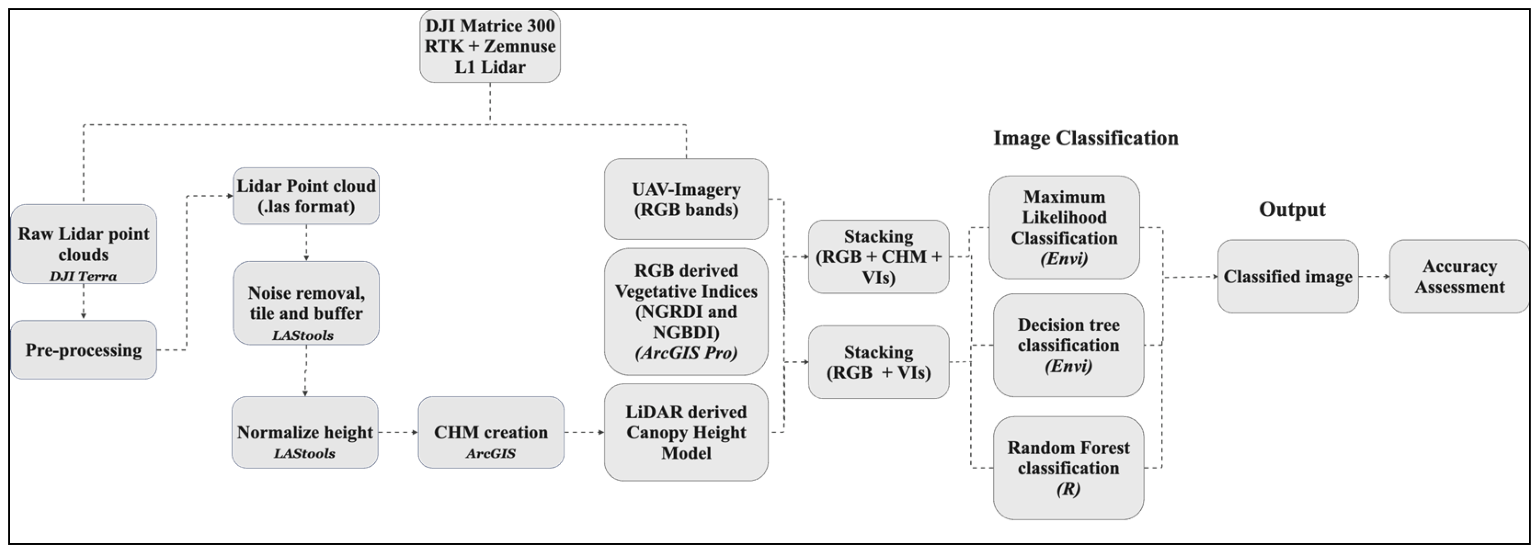
The study utilized two forms of remotely sensed data (UAV data)–LiDAR and RGB imagery. These data were captured using the DJI Matrice 300 (M300) Real-Time Kinematic (RTK) UAV equipped with the DJI Zenmuse L1 LiDAR sensor, which includes a Red–Green–Blue (RGB) camera. The DJI Pilot app was used to create and conduct flight missions. The M300 was flown at an altitude of 70 meters (230 feet) above ground level (AGL), with a speed of 5 m/s (11 mph), 70/60 percentage front and side overlap, 160 kHz point cloud sampling frequency, repetitive scanning mode, triple return/echo mode, and with elevation optimization and IMU calibration turned on. The Zenmuse L1 sensor requires centimeter-level positional data for point cloud data processing, which can be collected using either RTK or Post-Processed Kinematic (PPK) methods. For this study, RTK networks hosted by the Alabama Department of Transportation (ALDOT), Florida Department of Transportation (FDOT), and the eGPS RTK Network in Georgia were used for centimeter-level data collection. Storms occurred in January, March, and late August 2023. UAV surveys were conducted in March (Sites 1–2), late March–April (Sites 3–6), May (Sites 7–8), and December (Sites 9–10), with a temporal gap of approximately 8–16 weeks between storm occurrence and data collection. Figure 2 illustrates the overall workflow of the study.

2.3. Data Processing

2.3.1. LiDAR Data Pre-Processing and Derived Products

LiDAR data obtained from the DJI Zenmuse L1 was pre-processed using DJI Terra (v3.11.13.0), a proprietary software used to process LiDAR data for this sensor. The processing parameters were set to enable high-point cloud density and accuracy optimization, the output coordinate system was defined as WGS84/UTM zones, and the reconstruction output set to PNTS and LAS format. After successfully processing the data, a “.las” file containing the point cloud data was obtained.
LiDAR point cloud data (in “.las” format) were then processed to obtain normalized height, remove noise, and classify the ground using the LAStools [77] software. Functions used within LAStools included lasnoise to remove noise from the point cloud data, lastile to create tiles and buffers to prevent edge artifacts during data processing, and lasground classified the points as ground and non-ground. Lasground was executed with the nature option (optimal for natural and forested terrain), with all other parameters set to default values. Lasheight was then used to obtain normalized height (height above ground level), with height below 0 m and above the height of the tallest tree recorded during the field survey being filtered out. Lastile was used again to remove the buffer and lasmerge to merge the tiled LiDAR data. The obtained normalized point cloud data were processed using Esri ArcGIS Pro 3.1.0 [78] to generate a CHM. With point densities of approximately 651–1589 points/m2 (average spacing 2.5–3.5 cm; Appendix B: Table A1), CHMs were generated at a 2.5–3.5 cm grid size using the LAS Dataset to Raster tool in ArcGIS Pro with triangulation, natural neighbor interpolation, and cell size set to the average point spacing [33,39,79,80,81,82,83].

2.3.2. RGB Imagery Processing and Derived Products

The RGB imagery from the DJI Zenmuse L1 acquired with real-time RTK corrections was processed using ArcGIS Drone2Map (v2023.1.1) software, producing georeferenced orthomosaics. No additional radiometric calibration was applied. Two ratio-based RGB vegetation indices (Normalized Green Red Difference Index (NGRDI) [84] and Normalized Green Blue Difference Index (NGBDI)) [85] (Table 1) were created from each orthomosaic captured as single-date flights under stable midday illumination, following common practice in UAV-RGB applications [86,87,88,89]. NGBDI and NGRDI are two commonly used RGB-derived vegetative indices that are useful in detecting vegetation changes by highlighting the differences in the spectral signature of healthy, stressed, dead, or non-vegetated areas. Their values range from −1 to 1, with values closer to 1 indicating healthy vegetation and values closer to −1 indicating lower or no vegetation [84]. The vegetative indices were calculated using ArcGIS Pro 3.1.0.

2.4. Image Classification Scheme

Two datasets were created for the image classification process. The first dataset consisted of RGB bands, NGRDI, and NGBDI stacked together with LiDAR-derived CHM. Similarly, the second dataset included RGB imagery stacked with only vegetative indices NGRDI and NGBDI. The RGB imagery and its derived indices were resampled to match the spatial resolution of CHM before stacking. These two sets of data were then used separately as input for image classification, employing three different classification techniques: Random Forest (RF), Maximum Likelihood (ML), and Decision Tree (DT) classification.

2.4.1. Definition of Classification Criteria and Training Sample Collection

Given the site-specific environmental conditions, four distinct classification categories were defined: downed trees, standing trees, ground (non-trees), and water (where present). Soils on four of the sites were saturated at the time of sampling; therefore, the water class was included as a classification category only for those sites. Training samples were selected for each class at each study area based on visual interpretation of UAV imagery and site-based knowledge of the study area gained during the field visits. Training data and testing datasets were defined following the guidelines provided in Fundamentals of Remote Sensing [42].
For each site, 20 training ROIs and 14 validation (testing) ROIs were created per class using the ROI tool in ENVI (v5.6.2). Sites with three classes (downed trees, standing trees, and ground) contained 102 ROIs per site in total. Sites with water had four classes, resulting in a total of 136 ROIs per site (Table A2). The number of pixels per ROI varied with polygon size but followed the guideline of 10 m–100 m pixels per category (where m = number of bands used in the classification process), as recommended by Fundamentals of Remote Sensing [42]. This ensured that all classes, including minority classes such as downed trees, were adequately represented during classification. Class separability was assessed in ENVI using the ROI Separability tool, which calculates both Jeffries–Matusita (JM) and Transformed Divergence (TD) indices (0–2 scale) [90]. Classes with a spectral separability value of at least 1.9 were considered well-separated, and we used JM ≥ 1.9 as the threshold for this study [91]. Selection of the training samples and spectral separability was conducted in ENVI 5.6.2.

2.4.2. Image Classification

The first classification method used for the study was ML, a popular supervised classification method that requires training data [58,92,93]. An ML classifier assigns each pixel to a class based on the spectral and statistical properties of the training data. Unimodal statistics were derived from ROIs with spectral separability above 1.9, and the classification was then performed using ENVI. Default parametric settings were used for ML [37]. The probability threshold was set to default (0), so all pixels were assigned to the class with the highest discriminant. ENVI uses Maximum Likelihood classification to calculate the following discriminant functions for each pixel in the image [94,95].
g i x = l n   p ω i 1 2 l n Σ i 1 2 x m i T i 1 ( x m i )
where:
i = class
x = n-dimensional data (where n is the number of bands)
p( ω i ) = probability that class ω i occurs in the image and is assumed to be the same for all classes
| Σ i | = determinant of the covariance matrix of the data in class ω i
i 1   = its inverse matrix
m i = mean vector
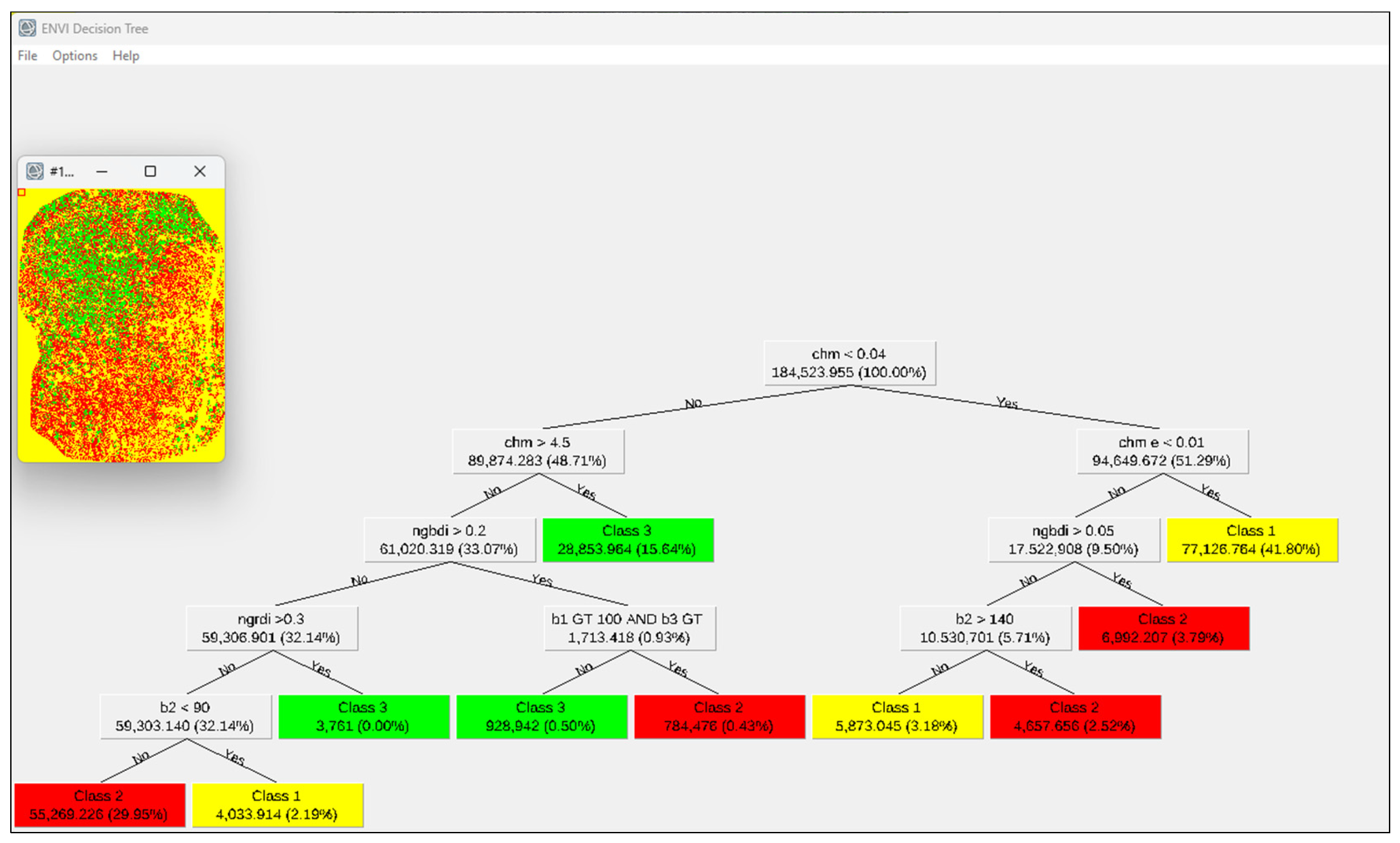
The second classification method used was DT and was also performed using ENVI (Figure 3). DT is a flexible and simple non-parametric classifier capable of multistage classification by utilizing a series of binary decisions to assign pixels into distinct classes [56,58]. With each new expression entered, a binary decision is generated, resulting in two new classes that can be divided into two more classes based on another expression [93]. These expressions or rules include thresholds on spectral bands and other auxiliary information, such as elevation [42]. Each band within each dataset was unique, necessitating careful analysis to determine the threshold for dividing pixels into different classes. The recorded values for each image band from the training data were carefully examined to find the appropriate thresholds required to classify pixels into distinct groups for conducting DT classification. By identifying distinct values within each class, specific threshold values were defined. Termination occurred at user-defined terminal class nodes. As trees were manually created, no automatic split criterion or pruning were applied.
The third approach used was RF [60], which was implemented using the R statistical software program (R Studio v2023.06.0). Instead of generating a single tree, this method builds a forest (or group) of trees by randomly selecting bootstrap samples from the training data and incorporating randomness into feature selection at each node split. The final prediction is made by majority voting across all trees, which minimizes variation and makes the algorithm less susceptible to overfitting [60,96]. This algorithm is an advantageous classification method due to its computational efficiency, noise insensitivity, and resistance to overfitting. In this study, RF was implemented using ModelMap, a comprehensive and user-centric R package [97]. ModelMap is specifically designed to streamline the processes of modeling and spatial mapping through a suite of functions such as model.build(), model.diagnostics(), model.mapmake(), model.importance.plot(), and model.interaction.plot() [97]. The predictor variables used were RGB imagery bands (Red (R), Green (G), and Blue(B)), NGRDI, NGBDI, and LiDAR-derived CHM. Key RF hyperparameters included the number of trees in the forest (ntree), number of predictor variables randomly selected at each split (mtry = (√p), where p = predictor variables), and minimum node size [43,63,92,98]. With six predictors (R, G, B, NGRDI, NGBDI, CHM), the hyperparameters were set at ntree = 500, mtry = 2, and nodesize = 1. RF can also determine the importance of each input variable [43], which is reported as both Mean Decrease Accuracy and Mean Decrease Gini. The same parameter settings were set across all ten sites for RF, ML, and DT.

2.4.3. Accuracy Assessment

To quantitatively analyze the classification performance of the three classifiers, ENVI software was utilized to create a confusion matrix for accuracy assessment using independent validation samples. ENVI’s ROI tool was used to create validation (testing) data. Testing ROIs were spatially independent from training ROIs and were separated by at least 5 m where feasible. The location information collected by the Trimble R2 GNSS receiver was utilized to guide the selection of the testing datasets. The same testing datasets were then used to evaluate RF, ML, and DT methods to ensure comparability. The performance of classification algorithms was measured and examined using key classification indicators from the confusion matrix, including Overall Accuracy (OA), kappa coefficient (k), producer’s accuracy (PA), and user’s accuracy (UA). OA indicates the proportion of correctly classified samples in the dataset. The kappa coefficient evaluates the agreement between observed and expected classification results by chance, with values ranging from −1 to 1. Here, 1 denotes full agreement, 0 denotes agreement equal to chance, while a value closer to −1 indicates agreement poorer than chance. PA is a measure that determines the likelihood that a specific class on the ground is accurately classified in the map or model. While UA is a measure that assesses the probability that the model-identified class represents that class on the ground [42].

3. Results

Using datasets that combined the LiDAR-derived CHM with RGB imagery, NGRDI, and NGBDI, the RF classifier consistently achieved the highest average accuracies, with an average OA of 94.52% and a kappa value of 0.92 (Table 2). ML demonstrated an average OA of 89.52% and an average kappa value of 0.85. The DT classifier performed less effectively than the other two methods, attaining an average OA of 81.78% and an average kappa value of 0.75. The findings were consistent across most sites, with RF outperforming ML and DT classifiers (Table 2). For instance, in Site 3, the highest OA (98.63%) and kappa coefficient (0.98) were achieved using the RF classifier. ML classification closely followed (OA = 93.34% and k = 0.90), whereas DT yielded OA (91.05%) and a kappa coefficient (0.87).
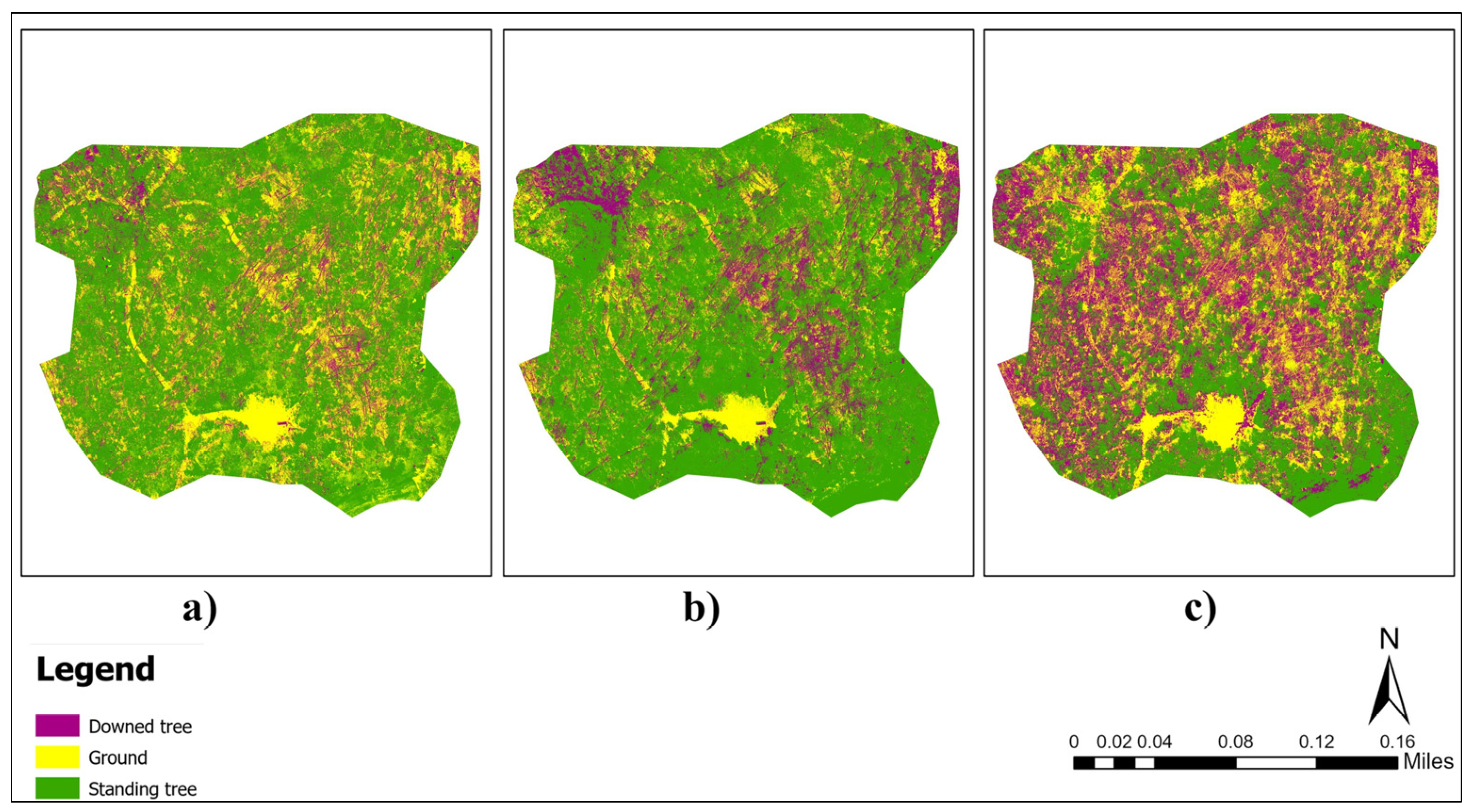
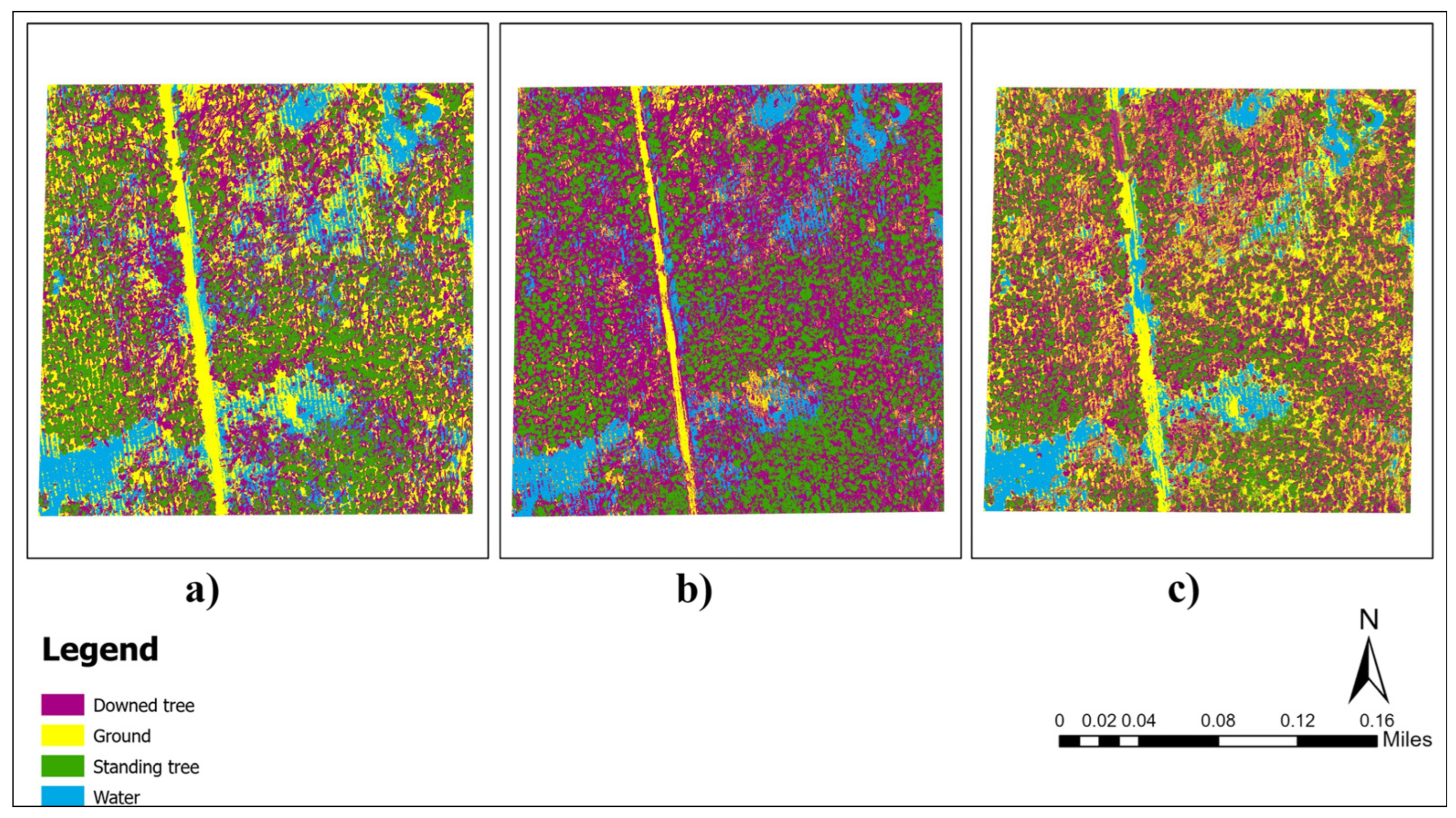
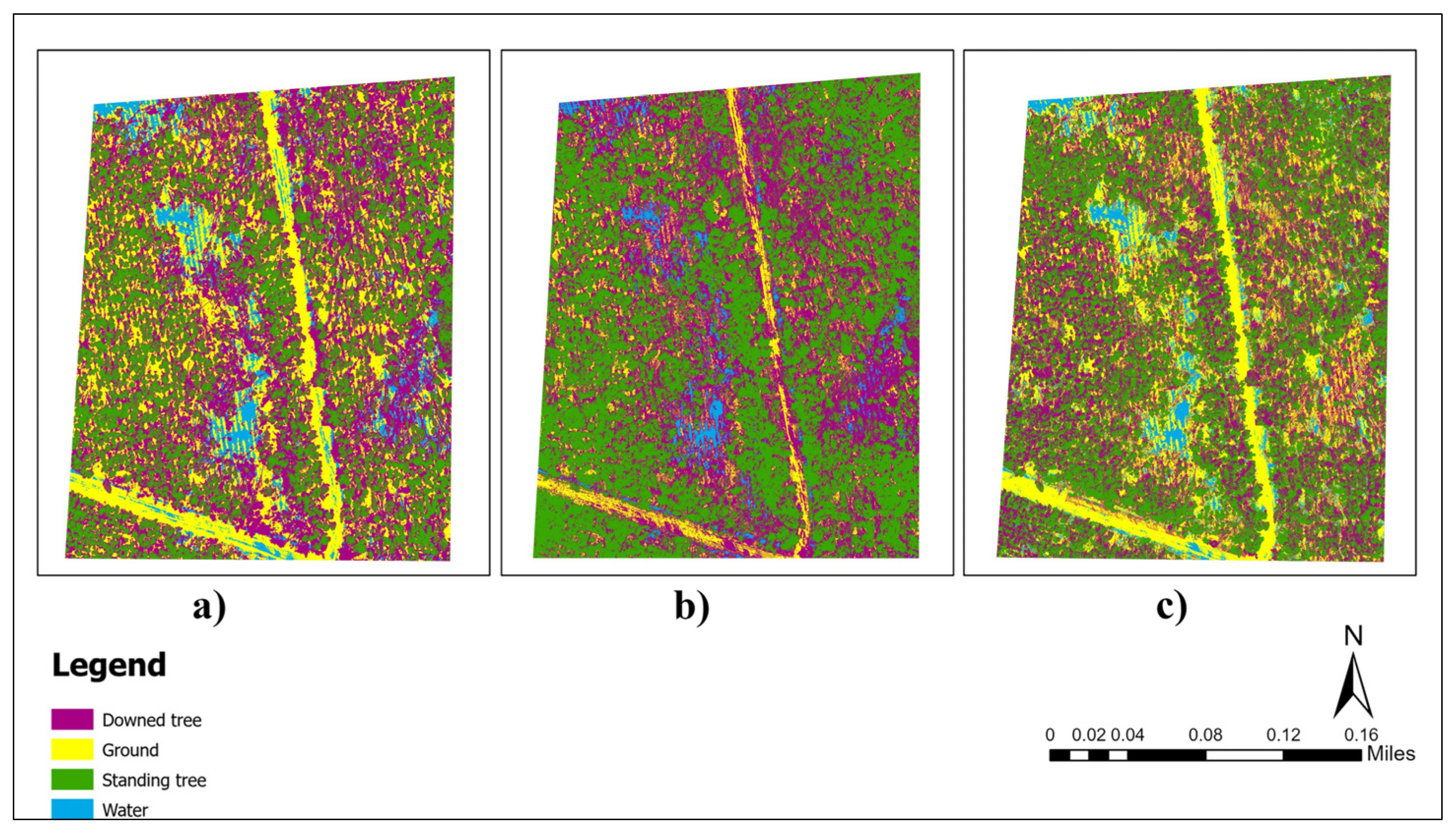
Damage classification maps were produced for all sites using the LiDAR-CHM integrated dataset and three classification algorithms: RF, ML, and DT. Figure 4 shows the classification map for Site 9, a representative map for the CHM-integrated dataset, showing four distinct categories: downed trees, standing trees, ground, and water. Classification maps for the remaining sites are provided in Appendix A (Figure A1, Figure A2, Figure A3, Figure A4, Figure A5, Figure A6, Figure A7, Figure A8, Figure A9, Figure A10, Figure A11, Figure A12, Figure A13, Figure A14, Figure A15, Figure A16, Figure A17 and Figure A18).
The performance of different classification methods without LiDAR-CHM (dataset with only RGB imagery combined with NGRDI and NGBDI) was also assessed. Without LiDAR-CHM, the OA and kappa coefficient declined for all classifiers (Table 2). RF remained the most accurate classifier, with an average OA of 77.56% and a kappa coefficient of 0.68. ML and DT followed, with average OAs of 74.64% and 62.51%, respectively, and corresponding kappa values of 0.64 and 0.47, respectively. The findings were consistent across most sites, with RF outperforming ML and DT classifiers. For instance, the highest OA (86.45%) and kappa coefficient (0.80) were obtained using RF in Site 2. The drop in classification accuracy in the absence of LiDAR-CHM was most noticeable for the DT classifier. For instance, at Site 7, the DT classifier’s OA decreased from 56.59% (with LiDAR-CHM) to 33.23% (without LiDAR-CHM).
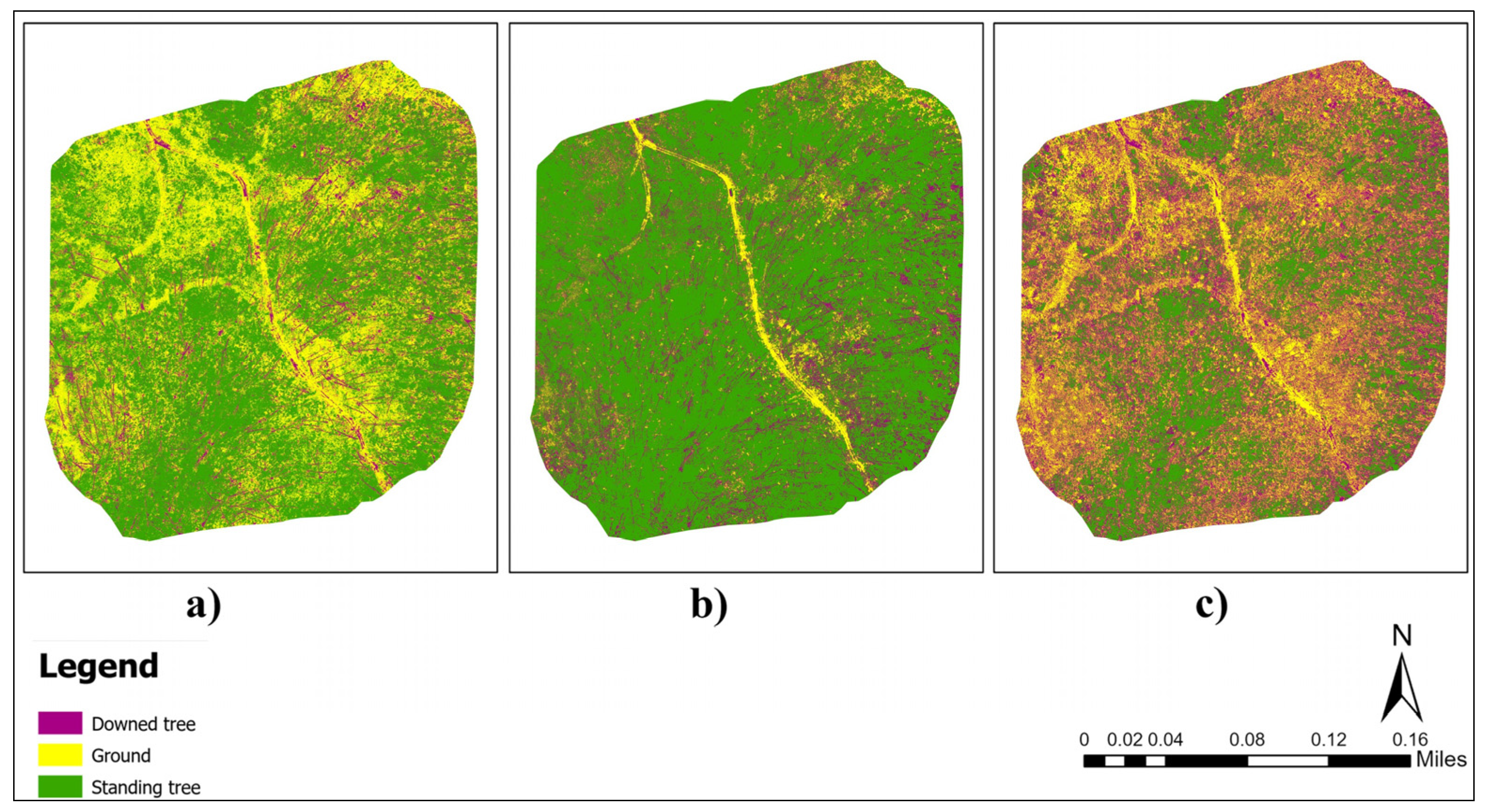
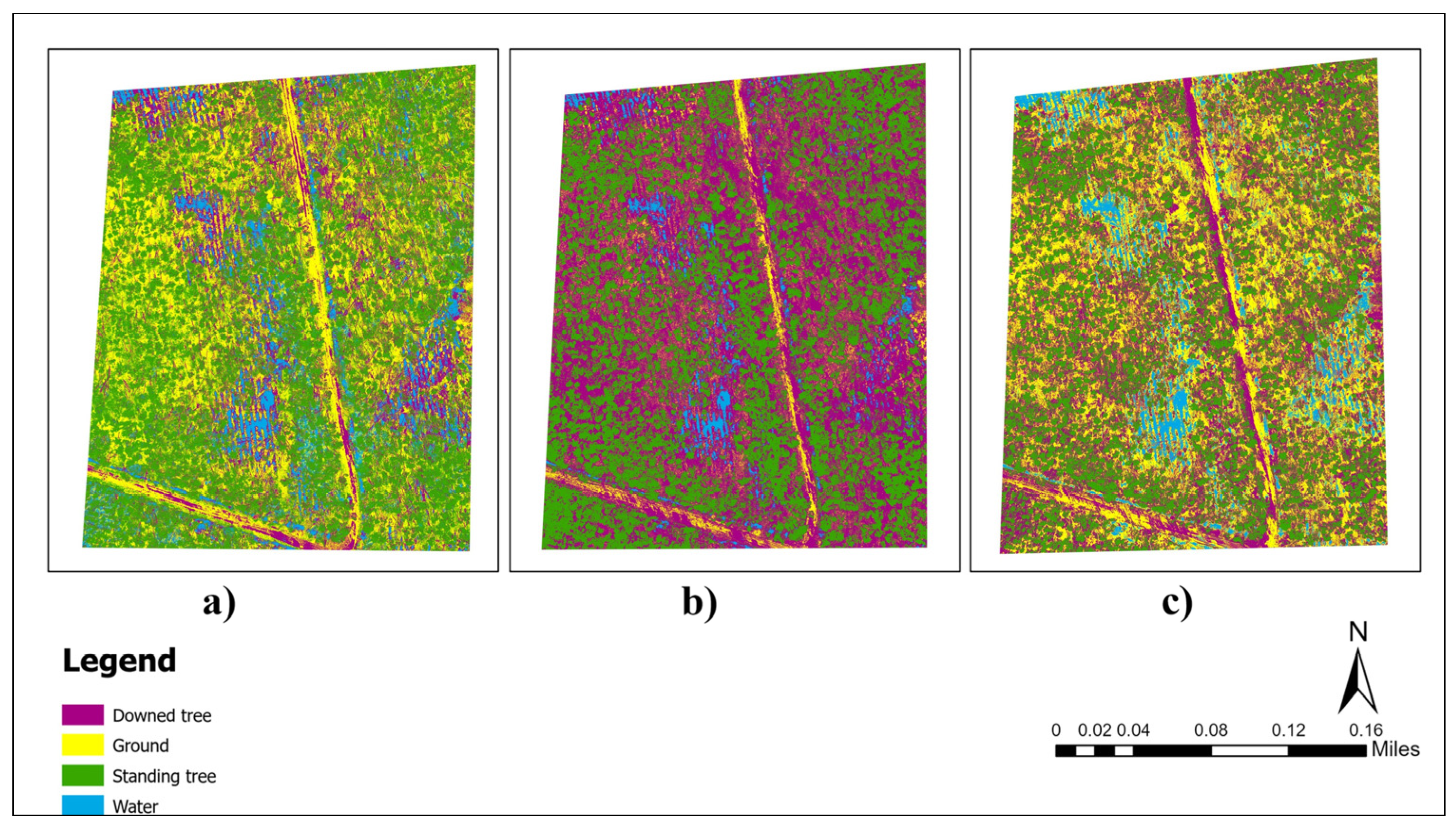
Damage classification maps for datasets without LiDAR-CHM (datasets with only RGB imagery combined with NGRDI and NGBDI) for all sites were also produced. Figure 5 shows the classification map for Site 9, a representative map without LiDAR-CHM, showing four distinct categories: downed trees, standing trees, ground, and water. This figure can be directly compared to Figure 4, which presents damage-classified maps prepared with LiDAR-CHM of the same site. Classification maps for the other sites can be found in Appendix A (Figure A1, Figure A2, Figure A3, Figure A4, Figure A5, Figure A6, Figure A7, Figure A8, Figure A9, Figure A10, Figure A11, Figure A12, Figure A13, Figure A14, Figure A15, Figure A16, Figure A17 and Figure A18).
PA and UA using the LiDAR-CHM integrated dataset for each classification category were obtained for each site (Table 3). Overall, RF consistently demonstrated the best accuracy, with the highest average PA for classifying ground (97.20%), downed trees (89.63%), and water (98.51%), indicating the classifier’s superior ability to label a true class correctly. Similarly, ML achieved an average PA of 85.08% for the ground class, 86.32% for the downed tree class, and 83.25% for the water class. Compared to ML, DT exhibited a slightly higher average PA of 85.25% for the ground class but lower for the downed tree (79.79%) and water (74.12%) classes. RF also produced the highest average UA for standing trees (98.34%) and downed trees (95.16%). Similarly, for the downed tree class, ML achieved an average UA of 85.36%, while DT achieved a UA of 73.86%, which is lower compared to the UA obtained by RF (95.16%) for the same class.
Using the dataset without LiDAR-CHM (based only on RGB imagery, NGRDI, and NGBDI), PA and UA were also assessed for each site (Table 4). In this case, ML demonstrated the best accuracy, with the highest average PA for classifying standing trees (83.94%) and downed trees (78.02%), as well as the highest average UA for standing trees (79.36%), ground (77.13%), and water (94.23%). The highest average PA for water (97.76%) was obtained with RF. Compared to the other two classifiers, DT showed the lowest overall PA (60.79%) and UA (51.39%) for classifying downed trees.
Confusion matrices were generated for each classification method across all ten sites, both with and without LiDAR-CHM, resulting in a total of 60 confusion matrices. Across all sites and classification methods, consistent patterns were observed in class confusion: standing trees were primarily misclassified as downed trees, while downed trees were commonly confused for ground, standing trees, or water classes. A detailed confusion matrix of RF classification, both with and without LiDAR-CHM for Site 9, is explained further as a representative example to illustrate the specific class confusion within the datasets (Table 5, Table 6, Table 7 and Table 8).
For Site 9 using the LiDAR-CHM dataset, RF correctly classified 305 out of 410 ground truth pixels as downed trees (Table 5). Hence, the PA for downed trees was 305/410 = 74.39%, which means that the classifier correctly identified 74.39% of the actual downed tree pixels. Downed trees had a total of 311 classified pixels, of which 305 were correctly classified by RF as downed trees, indicating that 98.07% (UA = 305/311) of the area labeled as downed trees in the classified image were downed trees on the ground. The most confused classes for RF in Site 9 were between water and downed trees, where 83 ground truth pixels of the downed tree class were incorrectly classified as water, followed by 17 pixels which were classified as standing trees, and 5 were classified as ground class, making omission error for the downed tree class (83+17+5/410 = 25.61%). Similarly, 6 standing tree truth pixels were classified as downed trees (6/311 = 1.93%) (Table 6).
Similarly, for Site 9, using the dataset without LiDAR-CHM, RF correctly classified 319 out of 388 ground truth pixels as downed trees, resulting in a PA of 82.22% (Table 7). Downed trees had a total of 418 classified pixels, of which 319 pixels were correctly classified by RF as downed trees, resulting in a UA of 76.32% (319/418). The most confused classes for RF were between downed trees and ground (48 pixels), followed by downed trees and water (13 pixels), and standing trees (8 pixels), making omission error for the downed tree class (48+13+8/388 = 17.78%). Similarly, 2 standing tree truth pixels were classified as downed trees, 96 pixels belonging to the ground class were classified as downed trees, and 1 water class ground truth pixel was classified as a downed tree (2+96+1/418 = 23.68%) (Table 8).
Incorporating CHM data improved classification accuracies across all three methods, as demonstrated by higher OA and k values (see Table 2). For example, Site 3 achieved an OA (98.63%) and k (0.98) for RF when LiDAR-CHM was included. This demonstrates a significant improvement compared to the performance without CHM, which had an OA of 71.32% and k of 0.56. This trend was consistent across all sites, highlighting the significance of CHM data in enhancing classification accuracy. On average, RF outperformed ML and DT, with corresponding kappa values following the trends in OA. RF classifier also showed high PA and UA for all tree damage categories when integrated with LiDAR-CHM data, particularly for standing trees and downed trees (Table 3 and Table 4). The ML classifier also performed well with datasets integrated with LiDAR-CHM, but had comparatively lower performance than RF.
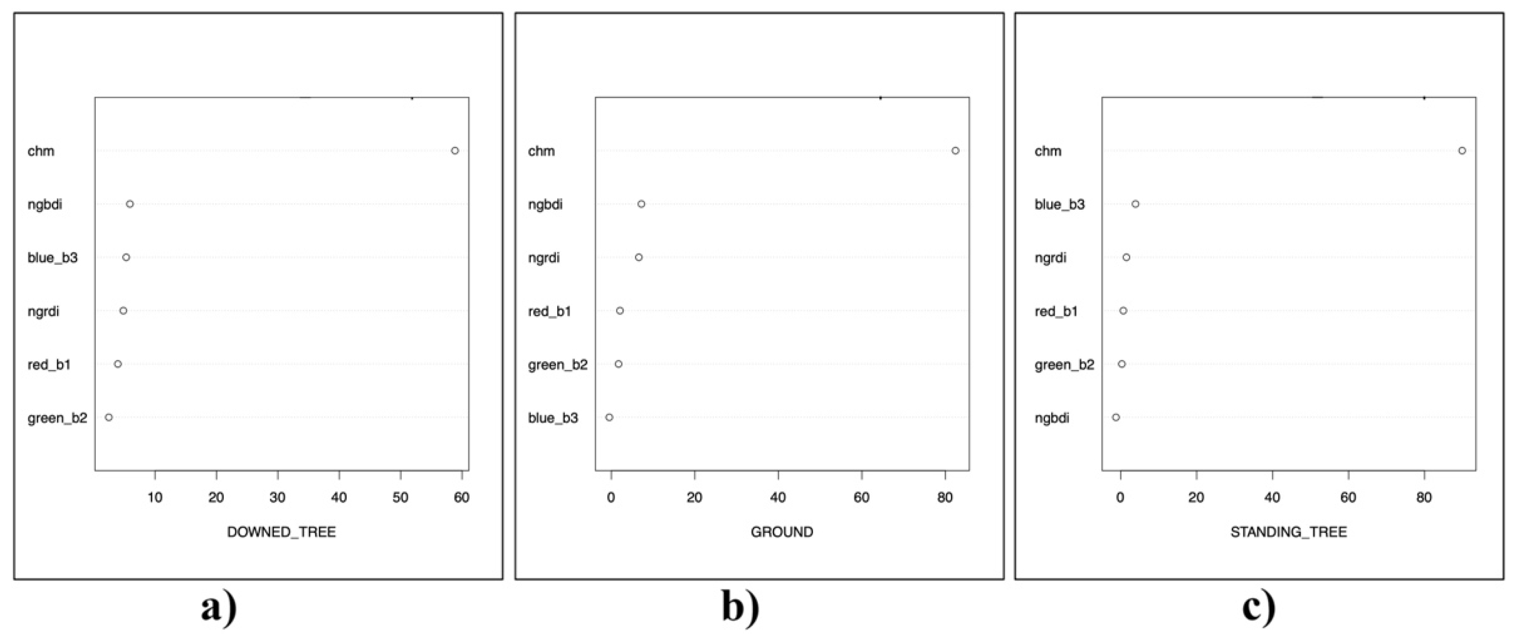
The RF model further provided insight into the importance of each input variable by ranking them in order of their significance in predicting the model’s accuracy. Figure 6 illustrates the variable importance plot for Site 1 using a dataset integrated with LiDAR-CHM, highlighting CHM as the most crucial variable for distinguishing between ground, downed trees, and standing trees. When comparing the role of variables across all ten sites, CHM remained the most influential variable across all four categories. The importance of spectral bands and indices (NGBDI, NGRDI, R, G, and B) varied depending on the category, with vegetative indices (NGDBI and NGRDI) having a secondary role compared to CHM.
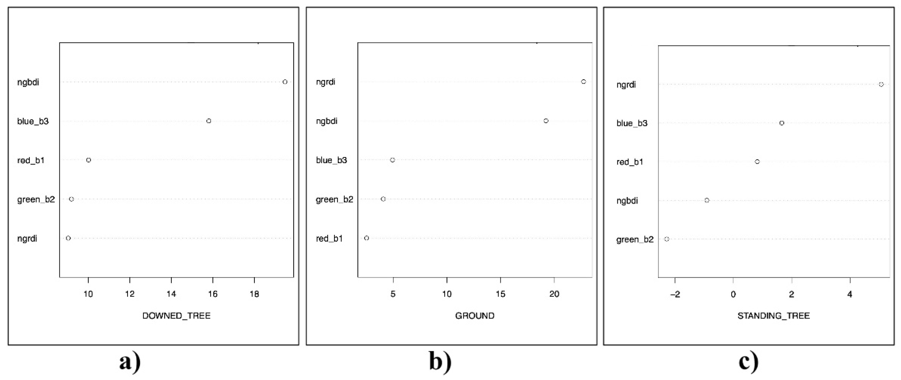
In the absence of LiDAR-CHM, vegetative indices (NGBDI and NGRDI) played a more significant role in classification. Figure 7 illustrates the variable importance plot for Site 1 using a dataset integrated without LiDAR-CHM, where NGBDI and NGRDI emerged as the two most crucial variables for distinguishing between ground, downed trees, and standing trees, as illustrated in all three plots. When comparing the role of variables across all ten sites, different spectral bands and indices had varying levels of importance depending on the category being predicted. Notably, NGRDI and NGBDI consistently emerged as the most influential variables across all four categories.
When variable importance was combined across all sites, CHM emerged as the dominant predictor, while vegetation indices (NGBDI, NGRDI) and RGB bands showed lower and more variable roles (Figure 8).

4. Discussion

This study explored the effectiveness of RF, ML, and DT techniques in classifying and mapping windstorm damage across Alabama, Georgia, and Florida. Each classification method was tested utilizing the combination of RGB bands, NGRDI, and NGBDI with and without LiDAR-CHM. The findings showed that the RF classifier outperformed ML and DT across several metrics, including OA, kappa coefficient, PA, and UA.
RF resulted in the best performance, both with the inclusion of LiDAR-CHM (average OA = 94.52%) and in its absence (average OA = 77.56%). These results align with prior research by [96,99], which highlights the effectiveness of machine learning techniques, particularly RF, in remote sensing applications. RF’s ability to handle multiple data types and complex feature sets makes it ideal for data fusion and classification tasks involving UAV-acquired datasets. This superiority is quantitatively supported by the higher OA and kappa values than ML and DT across most sites in this study. These findings are also consistent with [63], who emphasized the proficiency of the RF classifier in classifying environmental features. Ref [43] demonstrated the utility of UAV-RGB imagery and texture features in urban vegetation mapping, achieving classification accuracies of 90.6% and 86.2%. They also noted significant accuracy improvements when integrating texture features compared to using RGB data alone. Similarly, our study found that integrating CHM with RGB imagery and employing RF classification notably outperformed other methods (ML and DT), highlighting the robustness of this approach in handling varied and complex environmental datasets.
Ref. [51] successfully utilized RF within a Geographic Object-Based Image Analysis (GEOBIA) setup to identify coarse woody debris through high-resolution aerial images and LiDAR data. Their findings also noted that the combination of remote sensing data and advanced classification methods, such as RF, offers distinct advantages over traditional approaches like ML and DT algorithms when processing complex datasets. This has also been documented in studies by [63,92]. Moreover, Ref. [39] also provided support for the effectiveness of the RF classifier in handling intricate datasets, surpassing traditional methods like ISODATA clustering and ML with superior OA and kappa coefficient. In our analysis, ML achieved an average OA of 89.52% with CHM-included datasets and 74.64% without LiDAR-CHM. The DT classifier recorded an average OA of 81.78% with CHM datasets and 62.51% without LiDAR-CHM. These results indicate that integrating LiDAR-derived data improved classification accuracy across all three tested classification methods. Ref. [37] further supports this observation, showing that combining aerial imagery with LiDAR data significantly improves vegetation mapping accuracy. The insights on the importance of input variables, particularly the significance of CHM in distinguishing between classes, are consistent across studies by [73,100], emphasizing the critical role of structural data provided by LiDAR in environmental remote sensing applications.
Our study results highlight the substantial increase in classification accuracy with the inclusion of LiDAR-CHM. This improvement can be attributed to the combination of LiDAR-derived structural data with high-resolution RGB, where the structural features from LiDAR complement the spectral features from RGB in accurately classifying downed timber. This observation is consistent with [38,40], who reported the advantages of UAV–LiDAR in providing detailed three-dimensional information for precise identification and classification of features in forested landscapes. Our study’s high classification accuracy, especially for the RF (average OA of 94.52% with CHM and 77.56% without CHM), further validates the potential of combining LiDAR data with high-resolution RGB imagery for vegetation classification and post-disaster damage assessment. Ref. [99] underscored the effectiveness of employing UAVs equipped with LiDAR technology for detailed ecological classifications. Their research demonstrates the significant utility of RF in adeptly managing complex datasets captured via UAVs. Ref. [99] achieved a high OA of 83.3% using a fusion of features from all sensors (multispectral, hyperspectral, LiDAR, and thermal infrared imagery), highlighting the effectiveness of integrating multiple data types to enhance classification accuracy. Similarly, the study by Ref. [101] also supports the role of UAV–LiDAR technology in enhancing the precision and efficiency of environmental monitoring. Refs. [102,103] also noted that integrating CHM with spectral data improves detection of structural forest changes, mainly in damaged or complex areas, which is consistent with our findings.
The significance of LiDAR data in improving the accuracy of forest damage assessments has been highlighted by decreased model performance when CHM data were excluded from the analysis. This three-dimensional structural information provided by LiDAR plays a pivotal role in distinguishing between different forest damage categories, aligning with the findings of [27,50,52]. These studies emphasized the importance of LiDAR data in detecting downed logs and fallen trees, even in challenging environments. Ref. [50] in particular, focused on Object-Based Image Analysis (OBIA) combined with LiDAR data to detect and quantify downed logs in disturbed forest areas, demonstrating the significant aid of LiDAR-derived metrics in identifying and categorizing downed logs with approximately 73% accuracy. Our study similarly showed that including CHM data increased the average producer’s accuracy for classifying downed trees (78.03% to 89.63% accuracy).
Furthermore, the use of RGB-derived indices, such as the NGRDI and NGBDI, has been shown to enhance the differentiation between categories by increasing the contrast between living vegetation (standing trees) and non-vegetative materials (such as water and ground). This approach is supported by previous studies that have applied these indices to improve the classification and identification of vegetation classes, especially in studies utilizing UAVs. For example, Ref. [49] used a combination of the RF classification and NGRDI to automatically identify dead trees in UAV imagery captured using only an RGB sensor. The inclusion of NGRDI as an added feature improved the accuracy of detecting dead trees, achieving a confidence level of over 80% in identifying dead trees from UAV imagery. Similarly, the study by Ref. [104] demonstrated that vegetated areas could be differentiated using indices derived from the RGB bands of orthomosaic images. The authors suggested that combining various indices with CHM allows machine learning and deep learning algorithms to distinguish between different species of vegetation.
Our study further explored the difficulties in distinguishing between classes, especially when CHM data were excluded. The confusion between classes in the absence of CHM highlighted the need for advanced algorithms that could effectively utilize spectral and textural information to differentiate between closely related classes. Evaluation of the confusion matrix revealed significant misclassification between ground, water, and downed trees, as well as between downed and standing trees. This misclassification could be due to the presence of green leaves/needles on trees that were downed by windstorms, making it challenging to distinguish between downed and standing trees without CHM data. Additionally, the proximity of downed trees and water to the ground likely contributed to the confusion between these two classes. Ref. [105] also identified similar issues in land-cover classification, particularly confusion between water and bare land classes. They highlighted that the spectral properties of water pixels sometimes closely resembled those of bare land, especially in shadowed areas. In their study, confusion was also observed in differentiating the shrublands from herbaceous, mixed (deciduous), and bare lands, suggesting difficulties in distinguishing shrublands from adjacent land-cover types due to overlapping spectral signatures of the imagery. Furthermore, in the study by Ref. [48], there were instances where branches and objects with similar shapes were mistakenly identified as windthrown trees, revealing a limitation in distinguishing between tree trunks and similarly shaped objects.
During our study, we also encountered various logistical and technical challenges that impacted the data collection and processing phases. A key issue was maintaining active RTK status throughout UAV flights to ensure high-quality LiDAR data collection. The need for a reliable internet connection in rural areas was a persistent difficulty. To address this, we utilized portable WiFi hotspots that helped to improve internet connectivity for RTK operations and reduce disruptions. If cell service is an issue, a mobile base station receiver like the D-RTK 2 would be necessary [106]. Frequent weather changes, particularly strong gusts, created substantial challenges to RTK connectivity and UAV flight operations, often leading to delays. Ref. [89] also found that sudden weather changes, mainly wind gusts, made it difficult to conduct stable and reliable flights. To manage this, we conducted weather checks during the flight planning process and continuously monitored weather conditions using weather forecasting apps. Field data collection was further complicated due to the harsh site conditions, especially scattered debris from downed timber, which posed safety risks and slowed down the process than initially planned. The time between storm events and UAV surveys (8–16 weeks) may have impacted the detectability of downed trees, with the biggest concern being competing vegetation; decay was not a concern since it was still within the salvage harvest timeframe for storm-damaged trees [9,10]. Furthermore, processing the high-resolution LiDAR data from all study sites required substantial storage capacity and computational power. Upgrades to our data storage and processing infrastructure were essential, including the acquisition of more powerful computing systems to process large datasets efficiently. Despite these challenges, our study successfully applied UAV-based LiDAR and RGB imagery, showcasing the potential of these technologies in environmental monitoring and disaster management applications.
While this study highlighted the role of UAV–LiDAR and RGB integration, several limitations should be acknowledged. First, although equal ROI allocation across classes ensured minority classes (e.g., downed trees) were represented, misclassification errors remained, partly reflecting the spectral similarity of downed trees to canopy or soil, or ground. Future studies could examine class weighting or include more field-based reference plots to reduce such inaccuracies. Second, this study compared classifier performance using descriptive accuracy metrics rather than formal statistical tests, which is common practice in UAV–LiDAR studies [37,39,96,99]. The study compared classifier performance under consistent data processing and validation conditions across independent sites. Because each site had its own dataset and validation samples, tests such as McNemar’s or confidence intervals for OA were not included. Future studies with larger or combined datasets could include statistical testing to further support these comparisons. Third, models were trained separately for each site, which improved within-site accuracy but limits generalizability. Scaling to larger regions would require approaches such as combining multiple site data. Furthermore, because the analyses focused on single-date within-site classification, radiometric calibration was not performed; however, such calibration would be essential for multi-date or multi-sensor comparisons.

5. Conclusions

This study demonstrated the potential of combining UAV–LiDAR with UAV-derived RGB imagery for assessing windstorm damage on forest stands. By comparing three distinct classification techniques (ML, DT, and RF), insights were gained into the classification methods that could be utilized for efficient forest mapping and damage assessment. The RF technique emerged as the most effective method, offering superior accuracy and robustness using LiDAR-derived CHM and RGB imagery. These findings demonstrate the potential of RF in enhancing forest assessment in post-disaster settings. This study also emphasized the importance of combining spectral and structural data to improve the classification of storm-damaged forest stands. The results suggest that UAV-based approaches can be useful tools for post-storm forest assessment, providing detailed information that complements traditional field methods. However, our study did not assess economic implications, so these applications will need to be investigated further in the future.
Similarly, scaling to other forest types and regions was not evaluated in this study, and more research is needed to determine the application of these methodologies in diverse ecosystems and under varying storm conditions. In doing so, it would be useful to explore the inclusion of other remote sensing data, like hyperspectral, multispectral, or SAR, and their derivatives. These data sources may provide additional information, especially in areas with cloud cover, dense canopy, downed timber, and understory vegetation. Similarly, in this study, the downed tree class was sometimes misclassified as the standing tree class (particularly without LiDAR-CHM), and there was notable confusion between the downed tree, ground, and water classes. The use of integrated data from multiple sensors, such as RGB and NIR bands, along with advancements in image processing techniques and machine learning algorithms, can potentially provide solutions to the challenges of distinguishing among such closely related classification categories.
Future work can build on these findings by testing the approach across different storm events and forest conditions. It will also be important to explore how UAV–LiDAR data can be useful for determining the volume of damaged or fallen trees. This is crucial for efficient post-disaster restoration efforts. Computer vision algorithms can be employed to classify and segment the LiDAR point cloud data. These algorithms may be examined for distinguishing among varying levels of damage, identifying specific areas impacted by the storm, and accurately estimating the volume of downed timber.

Author Contributions

Conceptualization, D.B. and R.C.; methodology, D.B. and R.C.; formal analysis, D.B.; investigation, D.B.; data curation, D.B., A.R., and M.P.; writing (original draft preparation), D.B.; writing (review and editing), D.B., R.C., L.L.N., and S.K.; visualization, D.B.; supervision, R.C., L.L.N., and S.K.; project administration, D.B. and R.C.; funding acquisition, R.C. All authors have read and agreed to the published version of the manuscript.

Funding

This research was funded by the US Endowment for Forestry & Communities (G00015110).

Data Availability Statement

The data that support the findings of this study shall be made available from the corresponding author upon reasonable request.

Acknowledgments

Many thanks to the College of Forestry, Wildlife, and Environment at Auburn University for their continued support in enabling this research. Gratitude extends to Caroline Whiting and Trent Philips at the Department of Biosystems Engineering at Auburn University for the provision of essential equipment required for the fieldwork. We are equally thankful to all the county foresters and forest landowners who helped us with the search and access to the study sites. All UAV flights and fieldwork were conducted with prior permission from landowners and county foresters. No study sites were located within protected areas.

Conflicts of Interest

The authors declare no conflicts of interest. The funders had no role in the design of the study; in the collection, analyses, or interpretation of data; in the writing of the manuscript; or in the decision to publish the results.

Abbreviations

The following abbreviations are used in this manuscript:
USUnited States
UAVsUnmanned Aerial Vehicles
LiDARLight Detection and Ranging
RFRandom Forest
MLMaximum Likelihood
DTDecision Tree
CHMCanopy Height Model
SARSynthetic Aperture Radar
NWSNational Weather Service
DATDamage Assessment Toolkit
NOAANational Oceanic and Atmospheric Administration
NHCNational Hurricane Center
DbhDiameter at breast height
RTKReal-Time Kinematic
PPKPost-Processed Kinematic
ALDOTAlabama Department of Transportation
FDOTFlorida Department of Transportation
NGRDINormalized Green Red Difference Index
NGBDINormalized Green Blue Difference Index
ROIRegions of Interest
OAOverall Accuracy
PAProducer’s Accuracy
SVMSupport Vector Machines
UAUser’s Accuracy
GEOBIAGeographic Object-Based Image Analysis
OBIAObject-Based Image Analysis

Appendix A

This section consists of the damage classification maps for all other sites.
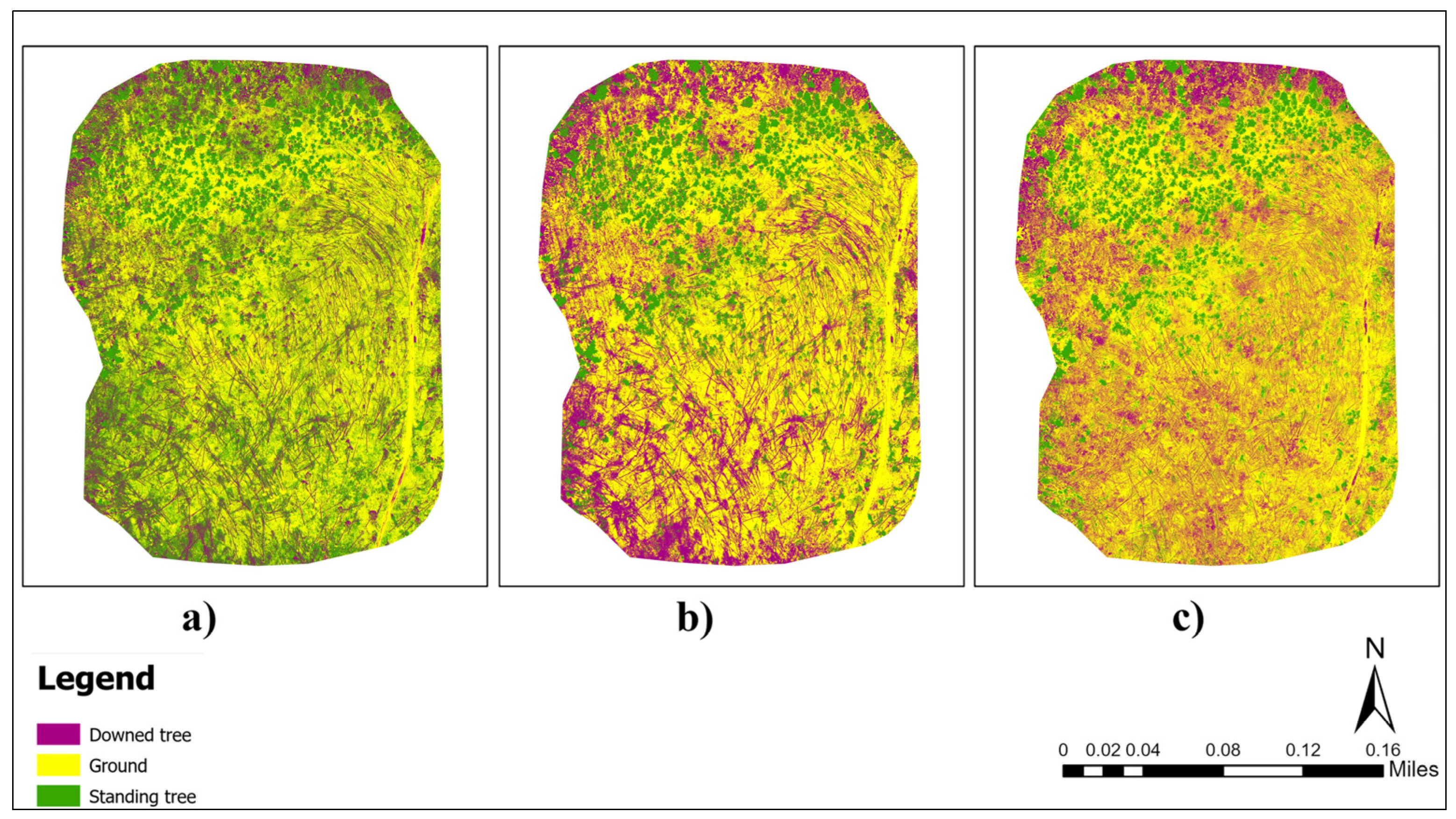
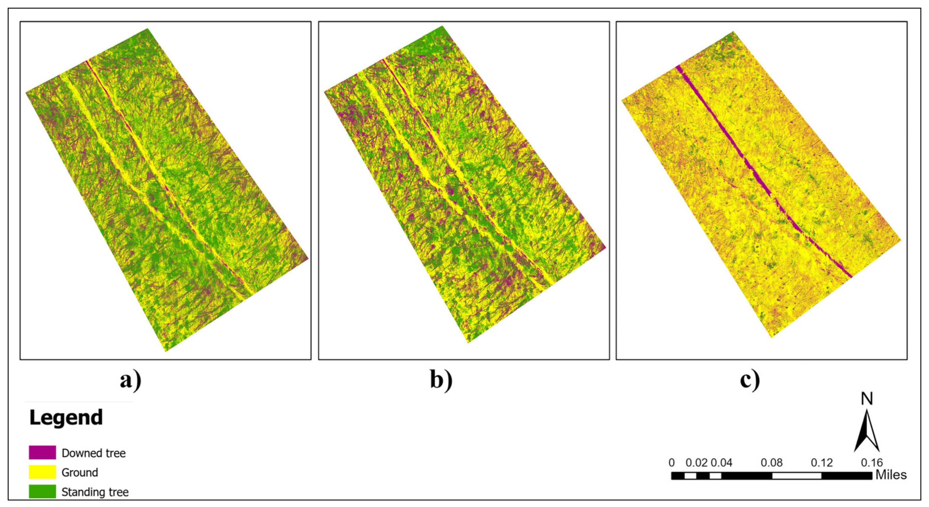
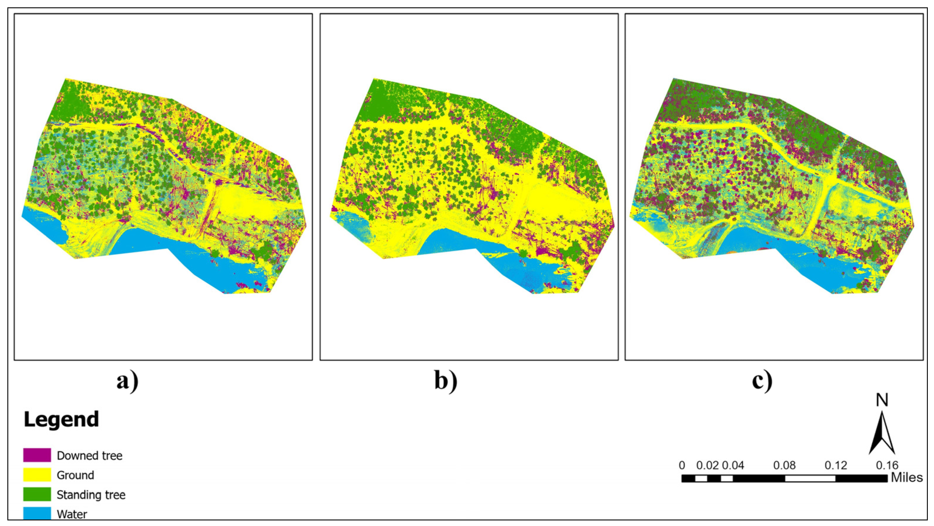
Figure A1. Map of the tornado-damaged site in Duncanville, Alabama (Site 1), prepared using a dataset integrated with LiDAR-CHM. Green represents standing trees, purple represents downed trees, and yellow represents the ground. Panel (a) represents RF classification, (b) represents ML classification, and (c) represents DT classification.
Drones 09 00756 g0a1
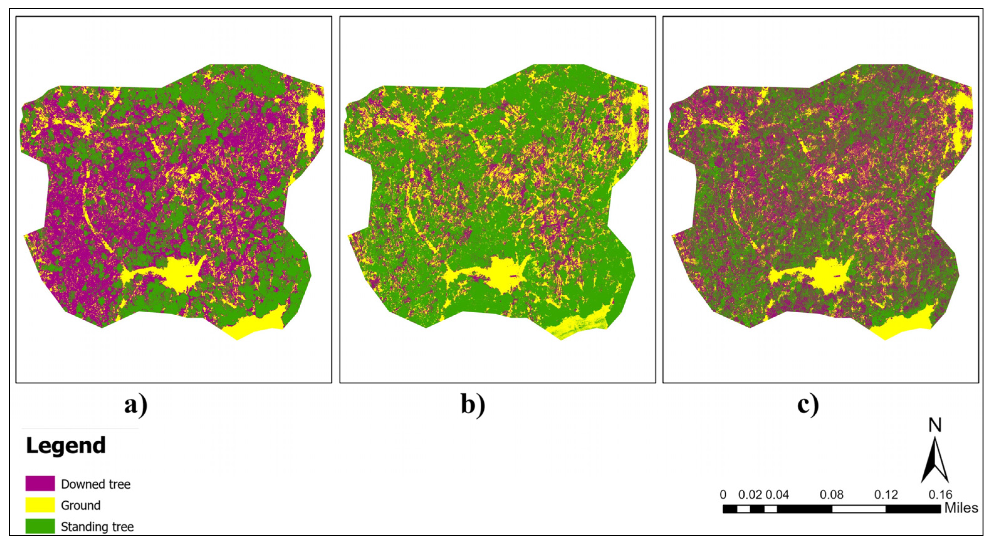
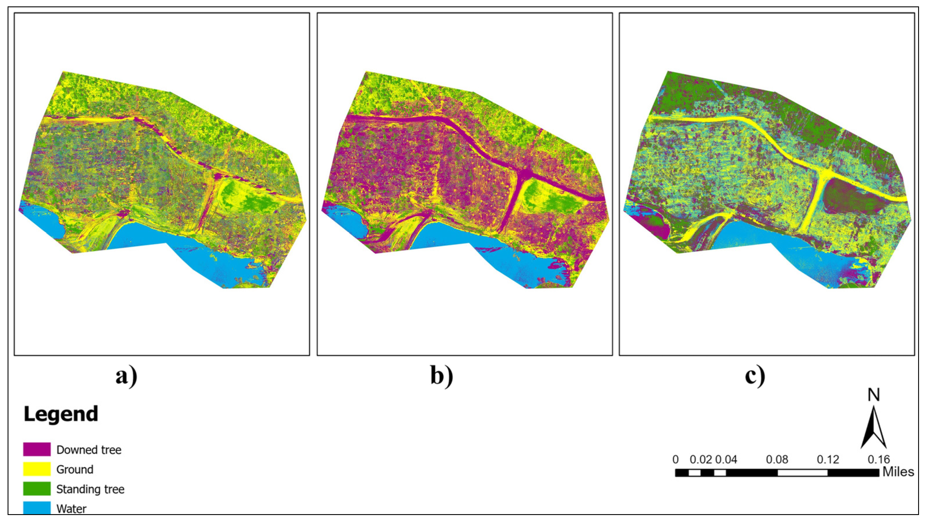
Figure A2. Map of the tornado-damaged site in Duncanville, Alabama (Site 1), prepared using a dataset integrated without LiDAR-CHM. Green represents standing trees, purple represents downed trees, and yellow represents the ground. Panel (a) represents RF classification, (b) represents ML classification, and (c) represents DT classification.
Drones 09 00756 g0a2
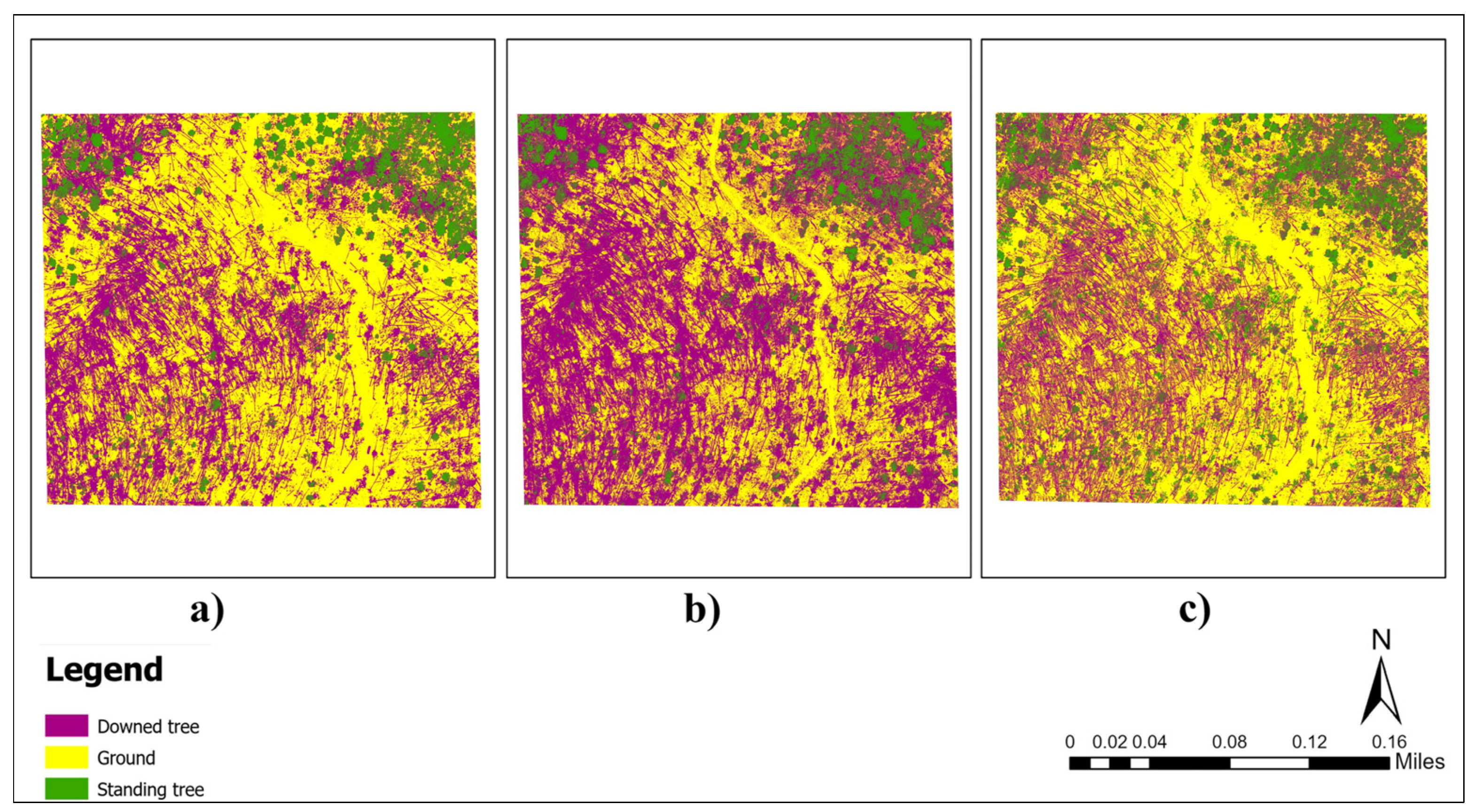
Figure A3. Map of tornado-damaged site in Duncanville, Alabama (Site 2), prepared using a dataset integrated with LiDAR-CHM. Green represents standing trees, purple represents downed trees, and yellow represents the ground. Panel (a) represents RF classification, (b) represents ML classification, and (c) represents DT classification.
Drones 09 00756 g0a3
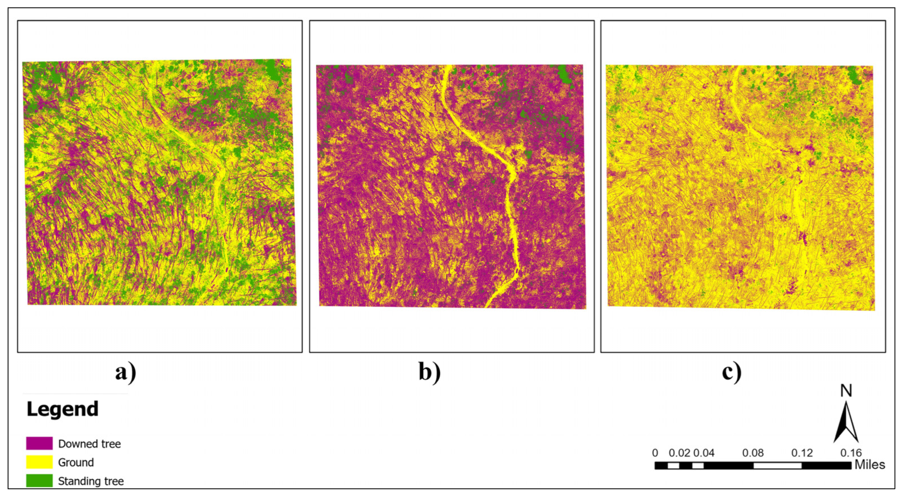
Figure A4. Map of the tornado-damaged site in Duncanville, Alabama (Site 2), prepared using a dataset integrated without LiDAR-CHM. Green represents standing trees, purple represents downed trees, and yellow represents the ground. Panel (a) represents RF classification, (b) represents ML classification, and (c) represents DT classification.
Drones 09 00756 g0a4
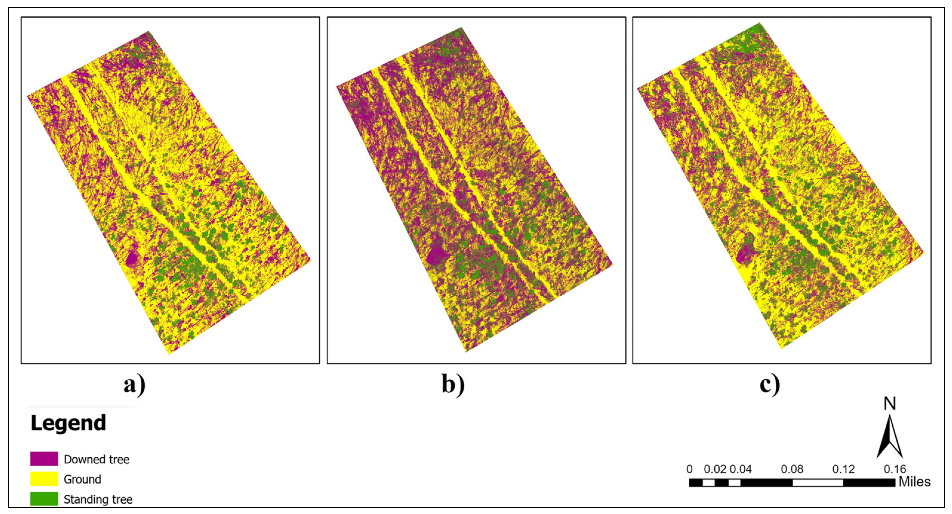
Figure A5. Map of the tornado-damaged site in Duncanville, Alabama (Site 3), prepared using a dataset integrated with LiDAR-CHM. Green represents standing trees, purple represents downed trees, and yellow represents the ground. Panel (a) represents RF classification, (b) represents ML classification, and (c) represents DT classification.
Drones 09 00756 g0a5
Figure A6. Map of the tornado-damaged site in Duncanville, Alabama (Site 3), prepared using a dataset integrated without LiDAR-CHM. Green represents standing trees, purple represents downed trees, and yellow represents the ground. Panel (a) represents RF classification, (b) represents ML classification, and (c) represents DT classification.
Drones 09 00756 g0a6
Figure A7. Map of the tornado-damaged site in Coosa, Alabama (Site 4), prepared using a dataset integrated with LiDAR-CHM. Green represents standing trees, purple represents downed trees, yellow represents the ground, and blue represents water. Panel (a) represents RF classification, (b) represents ML classification, and (c) represents DT classification.
Drones 09 00756 g0a7
Figure A8. Map of the tornado-damaged site in Coosa, Alabama (Site 4), prepared using a dataset integrated without LiDAR-CHM. Green represents standing trees, purple represents downed trees, yellow represents the ground, and blue represents water. Panel (a) represents RF classification, (b) represents ML classification, and (c) represents DT classification.
Drones 09 00756 g0a8
Figure A9. Map of the tornado-damaged site in Alexander City, Alabama (Site 5), prepared using a dataset integrated with LiDAR-CHM. Green represents standing trees, purple represents downed trees, and yellow represents the ground. Panel (a) represents RF classification, (b) represents ML classification, and (c) represents DT classification.
Drones 09 00756 g0a9
Figure A10. Map of the tornado-damaged site in Alexander City, Alabama (Site 5), prepared using a dataset integrated without LiDAR-CHM. Green represents standing trees, purple represents downed trees, and yellow represents the ground. Panel (a) represents RF classification, (b) represents ML classification, and (c) represents DT classification.
Drones 09 00756 g0a10
Figure A11. Map of the tornado-damaged site in Duncanville, Alabama (Site 6), prepared using a dataset integrated with LiDAR-CHM. Green represents standing trees, purple represents downed trees, and yellow represents the ground. Panel (a) represents RF classification, (b) represents ML classification, and (c) represents DT classification.
Drones 09 00756 g0a11
Figure A12. Map of the tornado-damaged site in Duncanville, Alabama (Site 6), prepared using a dataset integrated without LiDAR-CHM. Green represents standing trees, purple represents downed trees, and yellow represents the ground. Panel (a) represents RF classification, (b) represents ML classification, and (c) represents DT classification.
Drones 09 00756 g0a12
Figure A13. Map of the tornado-damaged site in Troup County, Georgia (Site 7), prepared using a dataset integrated with LiDAR-CHM. Green represents standing trees, purple represents downed trees, yellow represents the ground, and blue represents water. Panel (a) represents RF classification, (b) represents ML classification, and (c) represents DT classification.
Drones 09 00756 g0a13
Figure A14. Map of the tornado-damaged site in Troup County, Georgia (Site 7), prepared using a dataset integrated without LiDAR-CHM. Green represents standing trees, purple represents downed trees, yellow represents the ground, and blue represents water. Panel (a) represents RF classification, (b) represents ML classification, and (c) represents DT classification.
Drones 09 00756 g0a14
Figure A15. Map of the tornado-damaged site in Troup County, Georgia (Site 8), prepared using a dataset integrated with LiDAR-CHM. Green represents standing trees, purple represents downed trees, and yellow represents the ground. Panel (a) represents RF classification, (b) represents ML classification, and (c) represents DT classification.
Drones 09 00756 g0a15
Figure A16. Map of the tornado-damaged site in Troup County, Georgia (Site 8), prepared using a dataset integrated without LiDAR-CHM. Green represents standing trees, purple represents downed trees, and yellow represents the ground. Panel (a) represents RF classification, (b) represents ML classification, and (c) represents DT classification.
Drones 09 00756 g0a16
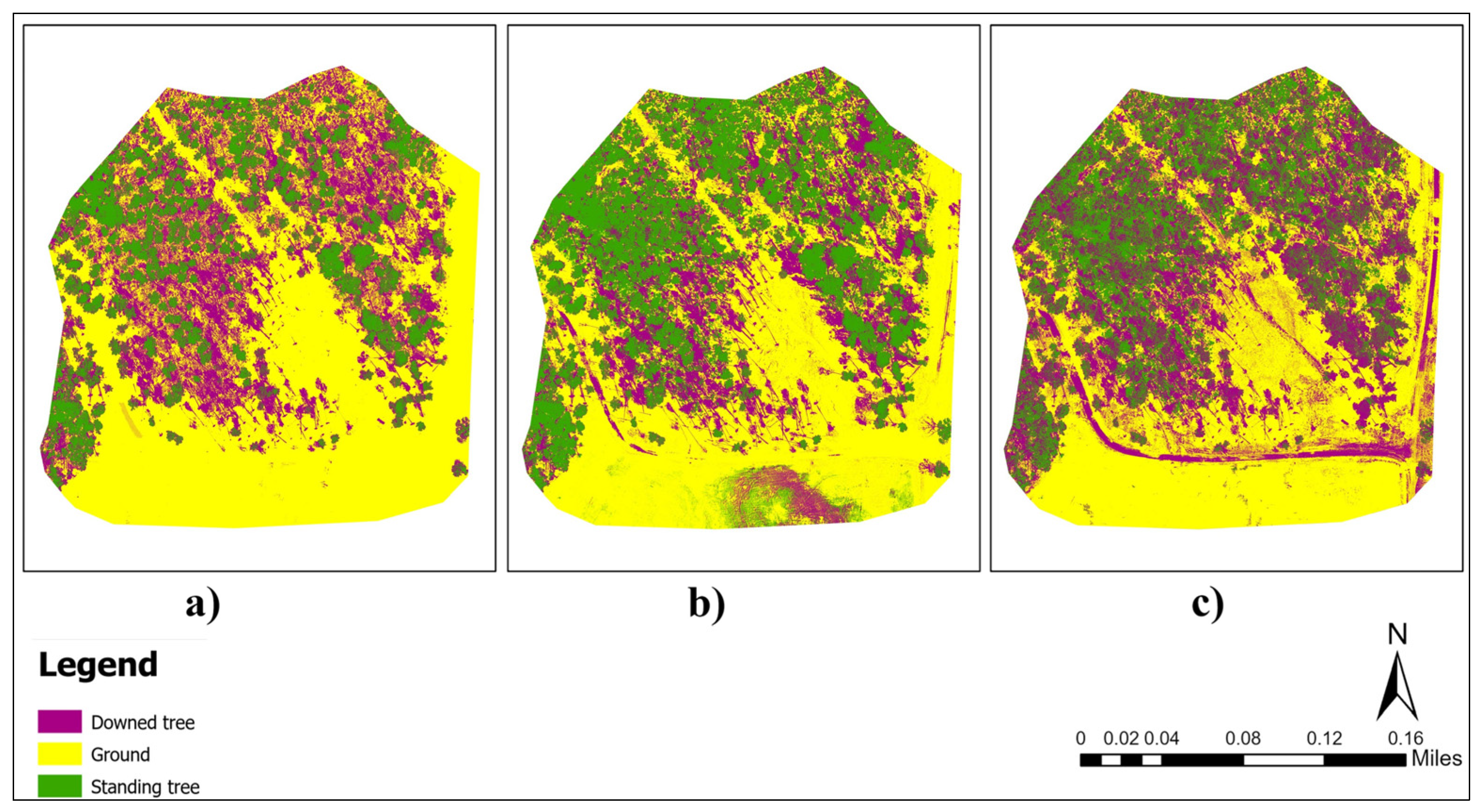
Figure A17. Map of the hurricane-damaged site in Perry, Florida (Site 10), prepared using a dataset integrated with LiDAR-CHM. Green represents standing trees, purple represents downed trees, and yellow represents the ground. Panel (a) represents RF classification, (b) represents ML classification, and (c) represents DT classification.
Drones 09 00756 g0a17
Figure A18. Map of the hurricane-damaged site in Perry, Florida (Site 10), prepared using a dataset integrated without LiDAR-CHM. Green represents standing trees, purple represents downed trees, and yellow represents the ground. Panel (a) represents RF classification, (b) represents ML classification, and (c) represents DT classification.
Drones 09 00756 g0a18

Appendix B

This section consists of the supplementary tables for a summary of LiDAR point density, point spacing, and the number of training and validation ROIs across the ten study sites.
Table A1. Summary of mean LiDAR point density (points/m2) and mean point spacing (m) derived from Zenmuse L1 flights across the ten study sites.
Site NumberMean Point Density (points/m2)Mean Point Spacing (m)
11057.430.03
2948.010.03
3713.570.03
4651.360.03
51048.690.03
6663.750.03
7978.930.03
8848.010.03
91191.070.02
101589.610.02
Table A2. Number of training and validation (testing) ROIs per class and per site.
Site NumberTraining ROIsValidation ROIsTotal
120*314*3102
220*314*3102
320*314*3102
420*414*4136
520*314*3102
620*314*3102
720*414*4136
820*314*3102
920*414*4136
1020*414*4136
Total6804761156

References

  1. Gardiner, B.; Blennow, K.; Carnus, J.M.; Fleischer, P.; Ingemarson, F.; Landmann, G.; Lindner, M.; Marzano, M.; Nicoll, B.; Orazio, C.; et al. Destructive Storms in European Forests: Past and Forthcoming Impacts. Final Report to European Commission—DG Environment; European Forest Institute: Joensuu, Finland, 2010. [Google Scholar]
  2. Mitchell, R.J.; Liu, Y.; O’Brien, J.J.; Elliott, K.J.; Starr, G.; Miniat, C.F.; Hiers, J.K. Future Climate and Fire Interactions in the Southeastern Region of the United States. For. Ecol. Manag. 2014, 327, 316–326. [Google Scholar] [CrossRef]
  3. Fortuin, C.C.; Montes, C.R.; Vogt, J.T.; Gandhi, K.J.K. Predicting Risks of Tornado and Severe Thunderstorm Damage to Southeastern U.S. Forests. Landsc. Ecol. 2022, 37, 1905–1919. [Google Scholar] [CrossRef]
  4. Sharma, A.; Ojha, S.K.; Dimov, L.D.; Vogel, J.G.; Nowak, J. Long-Term Effects of Catastrophic Wind on Southern US Coastal Forests: Lessons from a Major Hurricane. PLoS ONE 2021, 16, e0243362. [Google Scholar] [CrossRef]
  5. McNulty, S.G. Hurricane Impacts on US Forest Carbon Sequestration. Environ. Pollut. 2002, 116, S17–S24. [Google Scholar] [CrossRef]
  6. Mitchell, D.; Smidt, M.; McDonald, T.; Elder, T. Issues and Opportunities for Salvaging Storm Damaged Wood. In Proceedings of the 2021 ASABE Annual International Virtual Meeting, Online, 12–16 July 2021; American Society of Agricultural and Biological Engineers: St. Joseph, MI, USA, 2021. [Google Scholar]
  7. Forest Health Management Group; Georgia Forestry Commission. Hurricane Michael Timber Impacts Assessment, Georgia, October 10–11, 2018; Georgia Forestry Commission: Dry Branch, GA, USA, 2018. [Google Scholar]
  8. Georgia Forestry Commission. Hurricane Helene Recovery Assistance. Available online: https://gatrees.org/forest-management-conservation/natural-disaster-recovery/hurricane-helene-recovery-assistance/ (accessed on 29 September 2025).
  9. Bradley, S.; Maggard, A.; Carter, B.; Assessing and Managing Storm-Damaged Timber. Alabama A&M & Auburn Universities Extension Publication FOR-2066. 2018. Available online: https://www.aces.edu/wp-content/uploads/2018/12/FOR-2066.pdf (accessed on 22 November 2022).
  10. Musah, M.; Diaz, J.H.; Alawode, A.O.; Gallagher, T.; Peresin, M.S.; Mitchell, D.; Smidt, M.; Via, B. Field Assessment of Downed Timber Strength Deterioration Rate and Wood Quality Using Acoustic Technologies. Forests 2022, 13, 752. [Google Scholar] [CrossRef]
  11. Ritter, T.; Gollob, C.; Kraßnitzer, R.; Stampfer, K.; Nothdurft, A. A Robust Method for Detecting Wind-Fallen Stems from Aerial RGB Images Using a Line Segment Detection Algorithm. Forests 2022, 13, 90. [Google Scholar] [CrossRef]
  12. Windrim, L.; Bryson, M.; McLean, M.; Randle, J.; Stone, C. Automated Mapping of Woody Debris over Harvested Forest Plantations Using UAVs, High-Resolution Imagery, and Machine Learning. Remote Sens. 2019, 11, 733. [Google Scholar] [CrossRef]
  13. Dalponte, M.; Bruzzone, L.; Gianelle, D. Fusion of Hyperspectral and LIDAR Remote Sensing Data for Classification of Complex Forest Areas. IEEE Trans. Geosci. Remote Sens. 2008, 46, 1416–1427. [Google Scholar] [CrossRef]
  14. Guo, Q.; Su, Y.; Hu, T. LiDAR Principles, Processing and Applications in Forest Ecology; Academic Press: Cambridge, MA, USA, 2023. [Google Scholar]
  15. Lechner, A.M.; Foody, G.M.; Boyd, D.S. Applications in Remote Sensing to Forest Ecology and Management. One Earth 2020, 2, 405–412. [Google Scholar] [CrossRef]
  16. Bhardwaj, A.; Sam, L.; Akanksha; Martín-Torres, F.J.; Kumar, R. UAVs as Remote Sensing Platform in Glaciology: Present Applications and Future Prospects. Remote Sens. Environ. 2016, 175, 196–204. [Google Scholar] [CrossRef]
  17. Liebel, L.; Körner, M. Single-Image Super Resolution for Multispectral Remote Sensing Data Using Convolutional Neural Networks. Int. Arch. Photogramm. Remote Sens. Spat. Inf. Sci. 2016, XLI-B3, 883–890. [Google Scholar] [CrossRef]
  18. Mohan, M.; Leite, R.V.; Broadbent, E.N.; Wan Mohd Jaafar, W.S.; Srinivasan, S.; Bajaj, S.; Dalla Corte, A.P.; Do Amaral, C.H.; Gopan, G.; Saad, S.N.M.; et al. Individual Tree Detection Using UAV-Lidar and UAV-SfM Data: A Tutorial for Beginners. Open Geosci. 2021, 13, 1028–1039. [Google Scholar] [CrossRef]
  19. Villa, G.; Moreno, J.; Calera, A.; Amorós-López, J.; Camps-Valls, G.; Domenech, E.; Garrido, J.; González-Matesanz, J.; Gómez-Chova, L.; Martínez, J.Á.; et al. Spectro-Temporal Reflectance Surfaces: A New Conceptual Framework for the Integration of Remote-Sensing Data from Multiple Different Sensors. Int. J. Remote Sens. 2013, 34, 3699–3715. [Google Scholar] [CrossRef]
  20. Beland, M.; Parker, G.; Sparrow, B.; Harding, D.; Chasmer, L.; Phinn, S.; Antonarakis, A.; Strahler, A. On Promoting the Use of Lidar Systems in Forest Ecosystem Research. For. Ecol. Manag. 2019, 450, 117484. [Google Scholar] [CrossRef]
  21. Dassot, M.; Constant, T.; Fournier, M. The Use of Terrestrial LiDAR Technology in Forest Science: Application Fields, Benefits and Challenges. Ann. For. Sci. 2011, 68, 959–974. [Google Scholar] [CrossRef]
  22. Hudak, A.T.; Evans, J.S.; Stuart Smith, A.M. LiDAR Utility for Natural Resource Managers. Remote Sens. 2009, 1, 934–951. [Google Scholar] [CrossRef]
  23. Næsset, E.; Gobakken, T.; Holmgren, J.; Hyyppä, H.; Hyyppä, J.; Maltamo, M.; Nilsson, M.; Olsson, H.; Persson, Å.; Söderman, U. Laser Scanning of Forest Resources: The Nordic Experience. Scand. J. For. Res. 2004, 19, 482–499. [Google Scholar] [CrossRef]
  24. Silva, C.A.; Klauberg, C.; Hudak, A.T.; Vierling, L.A.; Fennema, S.J.; Corte, A.P.D. Modeling and Mapping Basal Area of Pinus taeda L. Plantation Using Airborne LiDAR Data. An. Acad. Bras. Ciênc. 2017, 89, 1895–1905. [Google Scholar] [CrossRef]
  25. Niemi, M.T.; Vauhkonen, J. Extracting Canopy Surface Texture from Airborne Laser Scanning Data for the Supervised and Unsupervised Prediction of Area-Based Forest Characteristics. Remote Sens. 2016, 8, 582. [Google Scholar] [CrossRef]
  26. Popescu, S.C. Estimating Biomass of Individual Pine Trees Using Airborne Lidar. Biomass Bioenergy 2007, 31, 646–655. [Google Scholar] [CrossRef]
  27. Tran, T.H.G.; Ressl, C.; Pfeifer, N. Integrated Change Detection and Classification in Urban Areas Based on Airborne Laser Scanning Point Clouds. Sensors 2018, 18, 448. [Google Scholar] [CrossRef] [PubMed]
  28. Abdollahnejad, A.; Panagiotidis, D.; Surový, P. Estimation and Extrapolation of Tree Parameters Using Spectral Correlation between UAV and Pléiades Data. Forests 2018, 9, 85. [Google Scholar] [CrossRef]
  29. Naesset, E. Determination of Mean Tree Height of Forest Stands Using Airborne Laser Scanner Data. ISPRS J. Photogramm. Remote Sens. 1997, 52, 49–56. [Google Scholar] [CrossRef]
  30. Nothdurft, A.; Gollob, C.; Kraßnitzer, R.; Erber, G.; Ritter, T.; Stampfer, K.; Finley, A.O. Estimating Timber Volume Loss Due to Storm Damage in Carinthia, Austria, Using ALS/TLS and Spatial Regression Models. For. Ecol. Manag. 2021, 502, 119714. [Google Scholar] [CrossRef]
  31. Xu, Z.; Li, W.; Li, Y.; Shen, X.; Ruan, H. Estimation of Secondary Forest Parameters by Integrating Image and Point Cloud-Based Metrics Acquired from Unmanned Aerial Vehicle. J. Appl. Remote Sens. 2020, 14, 022204. [Google Scholar] [CrossRef]
  32. d’Oliveira, M.V.; Broadbent, E.N.; Oliveira, L.C.; Almeida, D.R.; Papa, D.A.; Ferreira, M.E.; Zambrano, A.M.A.; Silva, C.A.; Avino, F.S.; Prata, G.A. Aboveground Biomass Estimation in Amazonian Tropical Forests: A Comparison of Aircraft-and Gatoreye UAV-Borne LIDAR Data in the Chico Mendes Extractive Reserve in Acre, Brazil. Remote Sens. 2020, 12, 1754. [Google Scholar] [CrossRef]
  33. Marcello, J.; Spínola, M.; Albors, L.; Marqués, F.; Rodríguez-Esparragón, D.; Eugenio, F. Performance of Individual Tree Segmentation Algorithms in Forest Ecosystems Using UAV LiDAR Data. Drones 2024, 8, 772. [Google Scholar] [CrossRef]
  34. Storch, M.; Jarmer, T.; Adam, M.; de Lange, N. Systematic Approach for Remote Sensing of Historical Conflict Landscapes with UAV-Based Laserscanning. Sensors 2022, 22, 217. [Google Scholar] [CrossRef]
  35. Almeida, D.R.A.; Broadbent, E.N.; Zambrano, A.M.A.; Wilkinson, B.E.; Ferreira, M.E.; Chazdon, R.; Meli, P.; Gorgens, E.B.; Silva, C.A.; Stark, S.C.; et al. Monitoring the Structure of Forest Restoration Plantations with a Drone-Lidar System. Int. J. Appl. Earth Obs. Geoinf. 2019, 79, 192–198. [Google Scholar] [CrossRef]
  36. Wallace, L.; Watson, C.; Lucieer, A. Detecting Pruning of Individual Stems Using Airborne Laser Scanning Data Captured from an Unmanned Aerial Vehicle. Int. J. Appl. Earth Obs. Geoinf. 2014, 30, 76–85. [Google Scholar] [CrossRef]
  37. Kim, J.; Popescu, S.C.; Lopez, R.R.; Wu, X.B.; Silvy, N.J. Vegetation Mapping of No Name Key, Florida Using Lidar and Multispectral Remote Sensing. Int. J. Remote Sens. 2020, 41, 9469–9506. [Google Scholar] [CrossRef]
  38. Liu, K.; Shen, X.; Cao, L.; Wang, G.; Cao, F. Estimating Forest Structural Attributes Using UAV-LiDAR Data in Ginkgo Plantations. ISPRS J. Photogramm. Remote Sens. 2018, 146, 465–482. [Google Scholar] [CrossRef]
  39. Thapa, N.; Narine, L.L.; Fan, Z.; Yang, S.; Tiwari, K. Detection of Invasive Plants Using NAIP Imagery and Airborne LiDAR in Coastal Alabama and Mississippi, USA. Ann. For. Res. 2023, 66, 63–77. [Google Scholar] [CrossRef]
  40. Corte, A.P.D.; Souza, D.V.; Rex, F.E.; Sanquetta, C.R.; Mohan, M.; Silva, C.A.; Zambrano, A.M.A.; Prata, G.; Alves De Almeida, D.R.; Trautenmüller, J.W.; et al. Forest Inventory with High-Density UAV-Lidar: Machine Learning Approaches for Predicting Individual Tree Attributes. Comput. Electron. Agric. 2020, 179, 105815. [Google Scholar] [CrossRef]
  41. Rijal, A.; Cristan, R.; Parajuli, M. Application of LiDAR in Forest Management. Available online: https://www.aces.edu/blog/topics/forestry/application-of-lidar-in-forest-management/ (accessed on 27 March 2024).
  42. Chuvieco, E. Fundamentals of Satellite Remote Sensing: An Environmental Approach; CRC Press: Boca Raton, FL, USA, 2020. [Google Scholar]
  43. Feng, Q.; Liu, J.; Gong, J. UAV Remote Sensing for Urban Vegetation Mapping Using Random Forest and Texture Analysis. Remote Sens. 2015, 7, 1074–1094. [Google Scholar] [CrossRef]
  44. Lu, B.; He, Y. Species Classification Using Unmanned Aerial Vehicle (UAV)-Acquired High Spatial Resolution Imagery in a Heterogeneous Grassland. ISPRS J. Photogramm. Remote Sens. 2017, 128, 73–85. [Google Scholar] [CrossRef]
  45. Poblete-Echeverría, C.; Olmedo, G.F.; Ingram, B.; Bardeen, M. Detection and Segmentation of Vine Canopy in Ultra-High Spatial Resolution RGB Imagery Obtained from Unmanned Aerial Vehicle (UAV): A Case Study in a Commercial Vineyard. Remote Sens. 2017, 9, 268. [Google Scholar] [CrossRef]
  46. Schiefer, F.; Kattenborn, T.; Frick, A.; Frey, J.; Schall, P.; Koch, B.; Schmidtlein, S. Mapping Forest Tree Species in High Resolution UAV-Based RGB-Imagery by Means of Convolutional Neural Networks. ISPRS J. Photogramm. Remote Sens. 2020, 170, 205–215. [Google Scholar] [CrossRef]
  47. Simpson, G.; Nichol, C.J.; Wade, T.; Helfter, C.; Hamilton, A.; Gibson-Poole, S. Species-Level Classification of Peatland Vegetation Using Ultra-High-Resolution UAV Imagery. Drones 2024, 8, 97. [Google Scholar] [CrossRef]
  48. Duan, F.; Wan, Y.; Deng, L. A Novel Approach for Coarse-to-Fine Windthrown Tree Extraction Based on Unmanned Aerial Vehicle Images. Remote Sens. 2017, 9, 306. [Google Scholar] [CrossRef]
  49. Lee, S.; Yu, B.-H. Automatic Detection of Dead Tree from UAV Imagery. In Proceedings of the 39th Asian Conference on Remote Sensing, Kuala Lumpur, Malaysia, 15–19 October 2018; pp. 15–19. [Google Scholar]
  50. Blanchard, S.D.; Jakubowski, M.K.; Kelly, M. Object-Based Image Analysis of Downed Logs in Disturbed Forested Landscapes Using Lidar. Remote Sens. 2011, 3, 2420–2439. [Google Scholar] [CrossRef]
  51. Lopes Queiroz, G.; McDermid, G.J.; Castilla, G.; Linke, J.; Rahman, M.M. Mapping Coarse Woody Debris with Random Forest Classification of Centimetric Aerial Imagery. Forests 2019, 10, 471. [Google Scholar] [CrossRef]
  52. Polewski, P.; Yao, W.; Heurich, M.; Krzystek, P.; Stilla, U. Detection of Fallen Trees in ALS Point Clouds Using a Normalized Cut Approach Trained by Simulation. ISPRS J. Photogramm. Remote Sens. 2015, 105, 252–271. [Google Scholar] [CrossRef]
  53. Polewski, P.; Yao, W.; Heurich, M.; Krzystek, P.; Stilla, U. A Voting-Based Statistical Cylinder Detection Framework Applied to Fallen Tree Mapping in Terrestrial Laser Scanning Point Clouds. ISPRS J. Photogramm. Remote Sens. 2017, 129, 118–130. [Google Scholar] [CrossRef]
  54. Asner, G.P.; Knapp, D.E.; Kennedy-Bowdoin, T.; Jones, M.O.; Martin, R.E.; Boardman, J.; Hughes, R.F. Invasive Species Detection in Hawaiian Rainforests Using Airborne Imaging Spectroscopy and LiDAR. Remote Sens. Environ. 2008, 112, 1942–1955. [Google Scholar] [CrossRef]
  55. Liang, W.; Abidi, M.; Carrasco, L.; McNelis, J.; Tran, L.; Li, Y.; Grant, J. Mapping Vegetation at Species Level with High-Resolution Multispectral and Lidar Data over a Large Spatial Area: A Case Study with Kudzu. Remote Sens. 2020, 12, 609. [Google Scholar] [CrossRef]
  56. Zhai, L.; Sun, J.; Sang, H.; Yang, G.; Jia, Y. Large area land cover classification with Landsat ETM+ images based on decision tree. Int. Arch. Photogramm. Remote Sens. Spatial Inf. Sci. 2012, XXXIX-B7, 421–426. [Google Scholar] [CrossRef]
  57. Otukei, J.R.; Blaschke, T. Land Cover Change Assessment Using Decision Trees, Support Vector Machines and Maximum Likelihood Classification Algorithms. Int. J. Appl. Earth Obs. Geoinf. 2010, 12, S27–S31. [Google Scholar] [CrossRef]
  58. Sharma, R.; Ghosh, A.; Joshi, P.K. Decision Tree Approach for Classification of Remotely Sensed Satellite Data Using Open Source Support. J. Earth Syst. Sci. 2013, 122, 1237–1247. [Google Scholar] [CrossRef]
  59. Balha, A.; Singh, C.K. Comparison of Maximum Likelihood, Neural Networks, and Random Forests Algorithms in Classifying Urban Landscape. In Application of Remote Sensing and GIS in Natural Resources and Built Infrastructure Management; Singh, V.P., Yadav, S., Yadav, K.K., Corzo Perez, G.A., Muñoz-Arriola, F., Yadava, R.N., Eds.; Springer International Publishing: Cham, Switzerland, 2022; pp. 29–38. ISBN 978-3-031-14096-9. [Google Scholar]
  60. Breiman, L. Random Forests. Mach. Learn. 2001, 45, 5–32. [Google Scholar] [CrossRef]
  61. Hamdi, Z.M.; Brandmeier, M.; Straub, C. Forest Damage Assessment Using Deep Learning on High Resolution Remote Sensing Data. Remote Sens. 2019, 11, 1976. [Google Scholar] [CrossRef]
  62. Ba, A.; Laslier, M.; Dufour, S.; Hubert-Moy, L. Riparian Trees Genera Identification Based on Leaf-on/Leaf-off Airborne Laser Scanner Data and Machine Learning Classifiers in Northern France. Int. J. Remote Sens. 2020, 41, 1645–1667. [Google Scholar] [CrossRef]
  63. Li, M.; Im, J.; Beier, C. Machine Learning Approaches for Forest Classification and Change Analysis Using Multi-Temporal Landsat TM Images over Huntington Wildlife Forest. GIScience Remote Sens. 2013, 50, 361–384. [Google Scholar] [CrossRef]
  64. Bandyopadhyay, M.; Van Aardt, J.A.N.; Cawse-Nicholson, K. Classification and Extraction of Trees and Buildings from Urban Scenes Using Discrete Return LiDAR and Aerial Color Imagery. In Laser Radar Technology and Applications XVIII, Proceedings of the SPIE—The International Society for Optical Engineering, Baltimore, MD, USA, 20 May 2013; Turner, M.D., Kamerman, G.W., Eds.; SPIE: St. Bellingham, WA, USA, 2013; Volume 8731, p. 873105. [Google Scholar]
  65. Li, B.; Hou, J.; Li, D.; Yang, D.; Han, H.; Bi, X.; Wang, X.; Hinkelmann, R.; Xia, J. Application of LiDAR UAV for High-Resolution Flood Modelling. Water Resour. Manag. 2021, 35, 1433–1447. [Google Scholar] [CrossRef]
  66. Secord, J.; Zakhor, A. Tree Detection in Urban Regions Using Aerial Lidar and Image Data. IEEE Geosci. Remote Sens. Lett. 2007, 4, 196–200. [Google Scholar] [CrossRef]
  67. Wang, X.; Wang, Y.; Zhou, C.; Yin, L.; Feng, X. Urban Forest Monitoring Based on Multiple Features at the Single Tree Scale by UAV. Urban For. Urban Green. 2021, 58, 126958. [Google Scholar] [CrossRef]
  68. Ferreira, M.P.; Dos Santos, D.R.; Ferrari, F.; Coelho, L.C.T.; Martins, G.B.; Feitosa, R.Q. Improving Urban Tree Species Classification by Deep-Learning Based Fusion of Digital Aerial Images and LiDAR. Urban For. Urban Green. 2024, 94, 128240. [Google Scholar] [CrossRef]
  69. Guimarães, N.; Pádua, L.; Marques, P.; Silva, N.; Peres, E.; Sousa, J.J. Forestry Remote Sensing from Unmanned Aerial Vehicles: A Review Focusing on the Data, Processing and Potentialities. Remote Sens. 2020, 12, 1046. [Google Scholar] [CrossRef]
  70. Kim, Y. Generation of Land Cover Maps through the Fusion of Aerial Images and Airborne LiDAR Data in Urban Areas. Remote Sens. 2016, 8, 521. [Google Scholar] [CrossRef]
  71. Zhong, H.; Zhang, Z.; Liu, H.; Wu, J.; Lin, W. Individual Tree Species Identification for Complex Coniferous and Broad-Leaved Mixed Forests Based on Deep Learning Combined with UAV LiDAR Data and RGB Images. Forests 2024, 15, 293. [Google Scholar] [CrossRef]
  72. Bork, E.W.; Su, J.G. Integrating LIDAR Data and Multispectral Imagery for Enhanced Classification of Rangeland Vegetation: A Meta Analysis. Remote Sens. Environ. 2007, 111, 11–24. [Google Scholar] [CrossRef]
  73. Shi, Y.; Skidmore, A.K.; Wang, T.; Holzwarth, S.; Heiden, U.; Pinnel, N.; Zhu, X.; Heurich, M. Tree Species Classification Using Plant Functional Traits from LiDAR and Hyperspectral Data. Int. J. Appl. Earth Obs. Geoinf. 2018, 73, 207–219. [Google Scholar] [CrossRef]
  74. Zabel, I.H.H.; Duggan-Hass, D.; Ross, R.M. The Teacher-Friendly Guide to Climate Change; Special publications; Paleontological Research Institution: Ithaca, NY, USA, 2017; ISBN 978-0-87710-519-0. [Google Scholar]
  75. United States Department of Agriculture; Natural Resources Conservation Services. Title 190-Forestry Inventory Methods Technical. 2018. Available online: https://directives.nrcs.usda.gov/sites/default/files2/1719592953/Forestry%20190-1%2C%20Forestry%20Inventory%20Methods.pdf (accessed on 26 April 2024).
  76. Northwest Natural Resource Group; Stewardship Forestry. Forest Inventory and Monitoring Guidelines; Northwest Certified Forestry: Seattle, WA, USA, 2014. [Google Scholar]
  77. Isenburg, Martin LAStools—Efficient LiDAR Processing Software (Version V2022.1); Rapidlasso GmbH: Gilching, Germany, 2023; Available online: https://rapidlasso.com/LAStools/ (accessed on 29 September 2025).
  78. ESRI ArcGIS Pro (Version 3.1.0); ESRI: Redlands, CA, USA, 2023. Available online: https://www.esri.com/en-us/arcgis/products/arcgis-pro/overview (accessed on 29 September 2025).
  79. Münzinger, M.; Prechtel, N.; Behnisch, M. Mapping the Urban Forest in Detail: From LiDAR Point Clouds to 3D Tree Models. Urban For. Urban Green. 2022, 74, 127637. [Google Scholar] [CrossRef]
  80. Guo, Q.; Li, W.; Yu, H.; Alvarez, O. Effects of Topographic Variability and Lidar Sampling Density on Several DEM Interpolation Methods. Photogramm. Eng. Remote Sens. 2010, 76, 701–712. [Google Scholar] [CrossRef]
  81. van Rees, E. Generating Digital Surface Models from Lidar Data in ArcGIS Pro. Available online: https://geospatialtraining.com/generating-digital-surface-models-from-lidar-data-in-arcgis-pro/ (accessed on 21 March 2024).
  82. ESRI Create DEMs and DSMs from Lidar Using a LAS Dataset. Available online: https://pro.arcgis.com/en/pro-app/latest/help/analysis/3d-analyst/create-dems-and-dsms-from-lidar.htm (accessed on 21 April 2024).
  83. rapidlasso Rasterizing Perfect Canopy Height Models from LiDAR. Available online: https://rapidlasso.de/rasterizing-perfect-canopy-height-models-from-lidar/ (accessed on 3 February 2024).
  84. Du, M.; Noguchi, N. Monitoring of Wheat Growth Status and Mapping of Wheat Yield’s within-Field Spatial Variations Using Color Images Acquired from UAV-Camera System. Remote Sens. 2017, 9, 289. [Google Scholar] [CrossRef]
  85. Zhang, X.; Zhang, F.; Qi, Y.; Deng, L.; Wang, X.; Yang, S. New Research Methods for Vegetation Information Extraction Based on Visible Light Remote Sensing Images from an Unmanned Aerial Vehicle (UAV). Int. J. Appl. Earth Obs. Geoinf. 2019, 78, 215–226. [Google Scholar] [CrossRef]
  86. Zheng, H.; Cheng, T.; Li, D.; Zhou, X.; Yao, X.; Tian, Y.; Cao, W.; Zhu, Y. Evaluation of RGB, Color-Infrared and Multispectral Images Acquired from Unmanned Aerial Systems for the Estimation of Nitrogen Accumulation in Rice. Remote Sensing 2018, 10, 824. [Google Scholar] [CrossRef]
  87. Shi, Y.; Gao, J.; Li, X.; Li, J.; Dela Torre, D.M.G.; Brierley, G.J. Improved Estimation of Aboveground Biomass of Disturbed Grassland through Including Bare Ground and Grazing Intensity. Remote Sens. 2021, 13, 2105. [Google Scholar] [CrossRef]
  88. Guimarães, M.J.M.; Reis, I.D.D.; Barros, J.R.A.; Lopes, I.; Da Costa, M.G.; Ribeiro, D.P.; Carvalho, G.C.; Da Silva, A.S.; Oliveira Alves, C.V. Identification of Vegetation Areas Affected by Wildfires Using RGB Images Obtained by UAV: A Case Study in the Brazilian Cerrado. Geomatics 2025, 5, 13. [Google Scholar] [CrossRef]
  89. Rijal, A.; Cristan, R.; Gallagher, T.; Narine, L.L.; Parajuli, M. Evaluating the Feasibility and Potential of Unmanned Aerial Vehicles to Monitor Implementation of Forestry Best Management Practices in the Coastal Plain of the Southeastern United States. For. Ecol. Manag. 2023, 545, 121280. [Google Scholar] [CrossRef]
  90. Sen, R.; Goswami, S.; Chakraborty, B. Jeffries-Matusita Distance as a Tool for Feature Selection. In Proceedings of the 2019 International Conference on Data Science and Engineering (ICDSE), Patna, India, 26–28 September 2019; IEEE: Piscataway, NJ, USA; pp. 15–20. [Google Scholar]
  91. Richards, J.A.; Jia, X. Remote Sensing Digital Image Analysis: An Introduction; Springer: Berlin/Heidelberg, Germany, 1999; ISBN 978-3-662-03980-9. [Google Scholar]
  92. Ok, A.O.; Akar, O.; Gungor, O. Evaluation of Random Forest Method for Agricultural Crop Classification. Eur. J. Remote Sens. 2012, 45, 421–432. [Google Scholar] [CrossRef]
  93. Sisodia, P.S.; Tiwari, V.; Kumar, A. A Comparative Analysis of Remote Sensing Image Classification Techniques. In Proceedings of the 2014 International Conference on Advances in Computing, Communications and Informatics (ICACCI), Delhi, India, 24–27 September 2014; pp. 1418–1421. [Google Scholar]
  94. Richards, J. Remote Sensing Digital Image Analysis; Springer: Berlin/Heidelberg, 1999; p. 240. [Google Scholar]
  95. NV5. Geospatial Software Maximum Likelihood Classification. Available online: https://www.nv5geospatialsoftware.com/docs/MaximumLikelihood.html (accessed on 29 September 2025).
  96. Fan, C.L. Ground Surface Structure Classification Using UAV Remote Sensing Images and Machine Learning Algorithms. Appl. Geomat. 2023, 15, 919–931. [Google Scholar] [CrossRef]
  97. Freeman, E.A.; Frescino, T.S.; Moisen, G.G. ModelMap: An R Package for Model Creation and Map Production. R Package Version 2018; U.S. Government Publishing Office: Washington, DC, USA, 2025; Volume 4, pp. 6–12. Available online: https://cran.r-project.org/web/packages/ModelMap/vignettes/VModelMap.pdf (accessed on 29 September 2025).
  98. Probst, P.; Wright, M.; Boulesteix, A.-L. Hyperparameters and Tuning Strategies for Random Forest. WIREs Data Min. Knowl. Discov. 2019, 9, e1301. [Google Scholar] [CrossRef]
  99. Hartling, S.; Sagan, V.; Maimaitijiang, M. Urban Tree Species Classification Using UAV-Based Multi-Sensor Data Fusion and Machine Learning. GIScience Remote Sens. 2021, 58, 1250–1275. [Google Scholar] [CrossRef]
  100. Qin, H.; Zhou, W.; Yao, Y.; Wang, W. Individual Tree Segmentation and Tree Species Classification in Subtropical Broadleaf Forests Using UAV-Based LiDAR, Hyperspectral, and Ultrahigh-Resolution RGB Data. Remote Sens. Environ. 2022, 280, 113143. [Google Scholar] [CrossRef]
  101. Van Alphen, R.; Rains, K.C.; Rodgers, M.; Malservisi, R.; Dixon, T.H. UAV-Based Wetland Monitoring: Multispectral and Lidar Fusion with Random Forest Classification. Drones 2024, 8, 113. [Google Scholar] [CrossRef]
  102. Balestra, M.; Marselis, S.; Sankey, T.T.; Cabo, C.; Liang, X.; Mokroš, M.; Peng, X.; Singh, A.; Stereńczak, K.; Vega, C.; et al. LiDAR Data Fusion to Improve Forest Attribute Estimates: A Review. Curr. For. Rep. 2024, 10, 281–297. [Google Scholar] [CrossRef]
  103. Gopalakrishnan, R.; Packalen, P.; Ikonen, V.-P.; Räty, J.; Venäläinen, A.; Laapas, M.; Pirinen, P.; Peltola, H. The Utility of Fused Airborne Laser Scanning and Multispectral Data for Improved Wind Damage Risk Assessment over a Managed Forest Landscape in Finland. Ann. For. Sci. 2020, 77, 97. [Google Scholar] [CrossRef]
  104. Srivastava, S.K.; Seng, K.P.; Ang, L.M.; Pachas, A.N.A.; Lewis, T. Drone-Based Environmental Monitoring and Image Processing Approaches for Resource Estimates of Private Native Forest. Sensors 2022, 22, 7872. [Google Scholar] [CrossRef]
  105. Tarasova, L.V.; Smirnova, L.N. Satellite-Based Analysis of Classification Algorithms Applied to the Riparian Zone of the Malaya Kokshaga River. IOP Conf. Ser. Earth Environ. Sci. 2021, 932, 012012. [Google Scholar] [CrossRef]
  106. Czyża, S.; Szuniewicz, K.; Kowalczyk, K.; Dumalski, A.; Ogrodniczak, M.; Zieleniewicz, Ł. Assessment of Accuracy in Unmanned Aerial Vehicle (UAV) Pose Estimation with the REAL-Time Kinematic (RTK) Method on the Example of DJI Matrice 300 RTK. Sensors 2023, 23, 2092. [Google Scholar] [CrossRef]
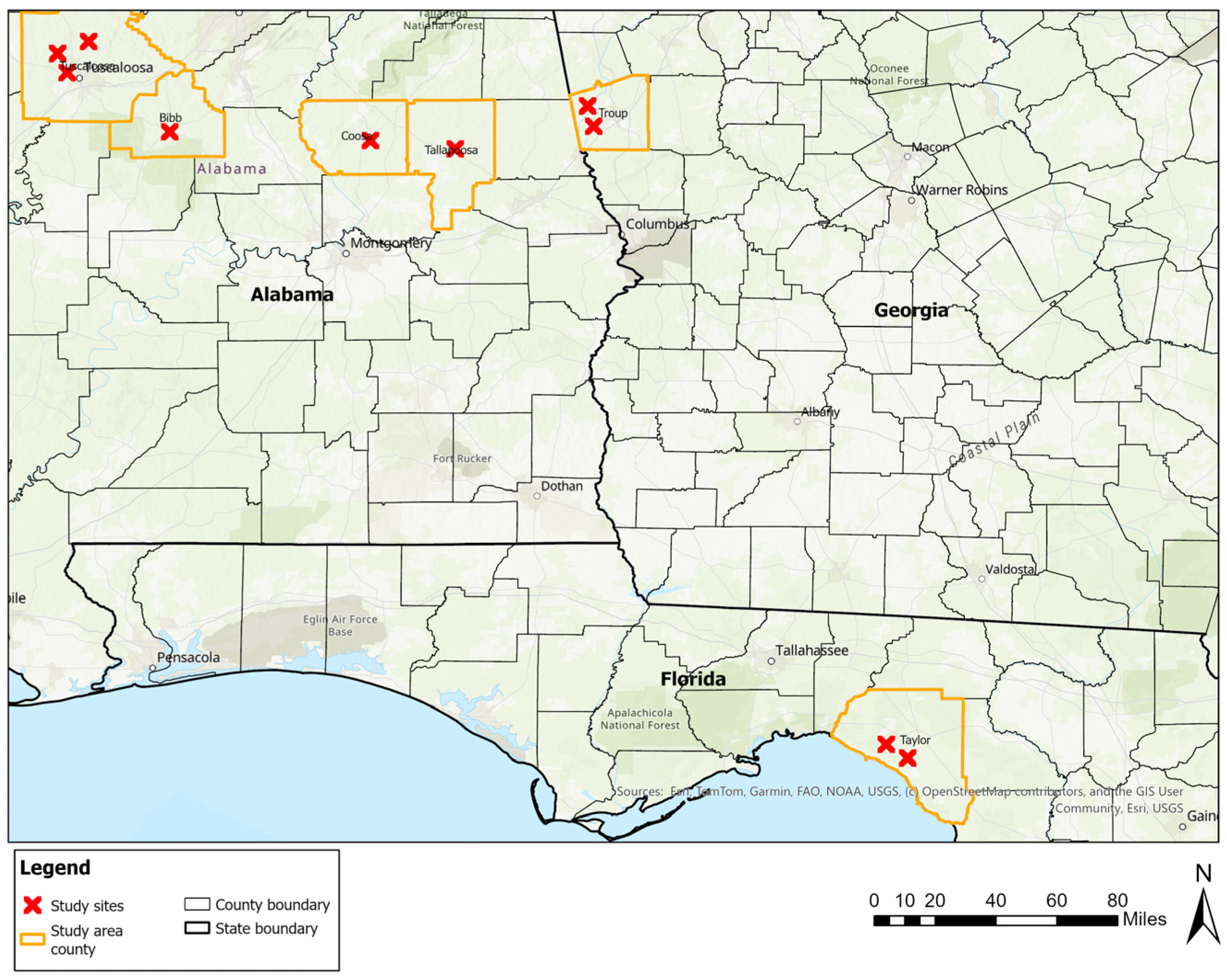
Figure 1. Study site locations.
Drones 09 00756 g001
Figure 2. Workflow of the study.
Drones 09 00756 g002
Figure 3. Decision Tree implementation in ENVI. The classification is divided into three categories: yellow (class 1) represents the ground class, red (class 2) represents downed trees, and green (class 3) represents standing trees.
Drones 09 00756 g003
Figure 4. Map of hurricane-damaged site in Perry, Florida (Site 9) prepared using a dataset integrated with LiDAR-CHM. Green represents standing trees, purple represents downed trees, yellow represents the ground, and blue represents water. Panel (a) represents RF classification, (b) represents ML classification, and (c) represents DT classification.
Drones 09 00756 g004
Figure 5. Map of hurricane-damaged site in Perry, Florida (Site 9) prepared using a dataset integrated without LiDAR-CHM. Green represents standing trees, purple represents downed trees, yellow represents the ground, and blue represents water. Panel (a) represents RF classification, (b) represents ML classification, and (c) represents DT classification.
Drones 09 00756 g005
Figure 6. Variable importance plots displaying the relative importance of each input variable for classifying windstorm damage using LiDAR-CHM integrated dataset (Site 1): (a) downed tree, (b) ground, (c) standing tree. The X-axis shows “Importance of input variables” and the Y-axis shows “Input variables/band used”.
Drones 09 00756 g006
Figure 7. Variable importance plots displaying the relative importance of each input variable for classifying windstorm damage using the dataset without LiDAR-CHM (Site 1): (a) downed tree, (b) ground, (c) standing tree. The X-axis shows “Importance of input variables” and the Y-axis shows “Input variables/band used”.
Drones 09 00756 g007
Figure 8. Boxplot of predictor importance across all sites: (a) with CHM-included datasets, where CHM shows consistently the highest importance compared to RGB bands and vegetation indices; (b) without CHM-included datasets, where vegetation indices (NGBDI, NGRDI) are most influential.
Drones 09 00756 g008
Table 1. Vegetation indices from RGB bands.
Vegetative IndicesFormula
Normalized Green Red Difference Index (NGRDI)(G − R)/(G + R)
Normalized Green Blue Difference Index (NGBDI)(G − B)/(G + B)
Table 2. Comparison of classification methods using CHM-included and CHM-excluded datasets for windstorm damage assessment. Classification accuracies (Overall Accuracy (OA) and kappa coefficient (k)) for each input dataset and method are presented.
SiteWith CHMWithout CHM
RFMLDTRFMLDT
OA (%)kOA (%)kOA (%)kOA (%)kOA (%)kOA (%)k
ALSite 195.040.9391.390.8792.870.8976.50.6582.540.7477.970.67
Site 294.790.9291.320.8789.870.8586.450.8082.160.7375.370.63
Site 398.630.9893.340.9091.050.8771.320.5680.680.7158.040.39
Site 498.080.9782.780.7781.240.7580.520.7466.690.5669.070.59
Site 593.930.9188.450.8386.890.8073.460.6062.980.4559.320.39
Site 695.450.9391.060.8794.990.9278.140.6767.590.5275.160.63
GESite 792.020.8986.690.8256.590.4269.410.5972.50.6333.230.11
Site 896.430.9586.940.8076.420.6576.830.6572.290.5945.360.18
FLSite 993.160.9191.550.8977.690.7083.010.7776.330.6870.860.61
Site 1087.640.8491.660.8970.150.6079.940.7382.680.7760.690.48
Average94.520.9289.520.8581.780.7577.560.6874.640.6462.510.47
Table 3. Comparison of accuracy using LiDAR-CHM integrated imagery in windstorm-affected sites. Classification accuracies (Producer’s Accuracy (PA) and User’s Accuracy (UA)) for each class and site are presented.
With CHM
MethodsSitePA (%)
(Standing Tree)
UA (%) (Standing Tree)PA (%) (Ground)UA (%) (Ground)PA (%)
(Downed Tree)
UA (%) (Downed Tree)PA (%)
(Water)
UA (%)
(Water)
198.1797.1995.4394.1191.4493.68
288.4098.0899.2397.9796.8789.33
Random397.30100.00100.0097.7898.3698.36
Forest499.7698.5899.7595.5196.4998.7296.2299.74
(RF)597.0098.4899.2788.4585.6895.92
695.3798.1095.9896.4495.0392.12
799.75100.0084.0892.1086.0396.6998.0782.02
899.31100.0098.2991.6791.897.76
998.5395.93100.0098.7674.3998.07100.0098.07
1071.5397.03100.0070.9280.2590.9399.7599.75
Average 94.5198.3497.2092.3789.6395.1698.5194.89
198.8391.5180.67100.0094.1885.14
2100.0092.5583.2198.8690.9184.09
Maximum394.2992.3591.9499.7393.9788.17
Likelihood
(ML)
499.5276.0167.4879.3184.0081.7579.9099.38
5100.0076.6396.3398.9969.4295.02
698.8492.2284.6397.0289.6285.19
7100.0096.6796.5267.3666.1899.6384.3096.14
8100.0094.5570.2289.5689.4678.12
998.5394.5891.7198.9293.4177.6982.60100.00
10100.0094.2788.1097.3792.0078.8086.21100.00
Average 99.0090.1385.0892.7186.3185.3683.2598.88
198.3395.4789.6394.6290.4188.59
298.5481.6295.2097.3075.6893.05
387.3986.0999.2498.0185.4887.89
Decision465.4677.2194.6287.9573.0063.7692.2198.66
Tree592.7581.1898.0491.5570.1588.65
(DT)696.0695.6295.9896.9093.0092.58
737.3568.1666.6753.3959.5645.0862.8070.84
857.8394.0181.3993.1890.6360.00
968.3084.2484.4276.3679.2764.7478.9291.74
1088.3278.4047.3577.8380.7554.2962.5682.74
Average 79.0384.2085.2586.7179.7973.8674.1285.99
Table 4. Comparison of accuracy using imagery without LiDAR-CHM in windstorm-affected sites. Classification accuracies (Producer’s Accuracy (PA) and User’s Accuracy (UA)) for each class for each site are presented.
Without CHM
MethodsSitePA (%)
(Standing Tree)
UA (%) (Standing Tree)PA (%) (Ground)UA (%) (Ground)PA (%)
(Downed Tree)
UA (%) (Downed Tree)PA (%)
(Water)
UA (%)
(Water)
176.6466.3259.8194.6493.5376.73
2100.0073.8095.8195.2463.7598.60
Random370.3374.5781.4666.3462.5473.19
Forest442.2875.2795.5869.9885.2479.9497.3598.51
(RF)585.8966.8261.2876.1274.1479.88
691.8471.7577.4785.2064.8879.85
763.9261.9652.6056.1766.1875.0894.0381.73
889.6981.0752.0480.9391.1271.30
990.8397.1561.4575.0982.2276.3299.6984.74
10100.0099.7038.6471.2082.1358.04100.0097.08
Average 81.1476.8467.6177.0976.5776.8997.7790.52
188.5679.4880.6397.9478.3673.60
288.6294.7479.6482.8778.3570.99
Maximum380.0885.4792.7170.1169.3590.32
Likelihood464.3171.5847.8164.0661.0143.1693.7999.37
(ML)572.6753.6637.8864.1579.6073.47
698.5463.4140.3879.4665.4867.69
758.8674.7044.2265.9590.1760.2395.1792.80
896.8873.2933.7982.1290.2668.18
998.2297.3637.1593.6695.3657.6373.9984.75
1092.66100.0069.3271.0072.3364.6997.30100.00
Average 83.9479.3756.3577.1378.0367.0190.0694.23
193.4377.1172.6492.0267.6667.66
282.4697.8185.0361.2158.5477.11
348.5895.2269.6044.2160.6852.27
Decision444.9281.5653.3555.9684.2356.4993.2094.03
Tree555.5664.0140.3965.0282.4754.36
(DT)680.7689.6461.5483.9084.2360.60
733.8640.6834.9730.404.914.4258.8165.92
842.8180.5939.5147.3953.8733.57
989.3596.4941.3449.5057.7352.58100.0087.53
1087.1657.8152.2162.5453.6054.8750.7573.16
Average 65.8978.0955.0659.2260.7951.3975.6980.16
Table 5. Confusion matrix for RF using dataset integrated with LiDAR-CHM for Site 9 (in pixels).
Ground Truth (Pixels)
ClassStanding TreeDowned TreeGroundWaterTotal
Standing tree4011700418
Downed tree630500311
Ground053980403
Water0830408491
Total4074103984081623
Table 6. Error of Commission and Omission obtained for RF using the dataset integrated with LiDAR-CHM for Site 9.
ClassCommission (%)Omission (%)Commission (Pixels)Omission (Pixels)
Standing tree4.071.4717/4186/407
Downed tree1.9325.616/311105/410
Ground1.240.005/4030/398
Water16.900.0083/4910/408
Table 7. Confusion matrix for RF using the dataset integrated without LiDAR-CHM for Site 9 (in pixels).
Ground Truth (Pixels)
ClassStanding TreeDowned TreeGroundWaterTotal
Standing tree307810316
Downed tree2319961293
Ground25482200380
Water41341322418
Total3383883583231407
Table 8. Error of Commission and Omission obtained for RF using the dataset integrated without LiDAR-CHM for Site 9.
ClassCommission (%)Omission (%)Commission (Pixels)Omission (Pixels)
Standing tree2.859.179/31631/338
Downed tree23.6817.7899/41869/388
Ground24.9138.5573/293138/358
Water15.260.3158/3801/323
Disclaimer/Publisher’s Note: The statements, opinions and data contained in all publications are solely those of the individual author(s) and contributor(s) and not of MDPI and/or the editor(s). MDPI and/or the editor(s) disclaim responsibility for any injury to people or property resulting from any ideas, methods, instructions or products referred to in the content.