Highlights
What are the main findings?
- A globally applicable definition of the grid coordinate system with a smoothly varying north direction was presented and a formula for the grid azimuth along a great ellipse route was derived based on the proposed grid frame.
- A high-precision flight guidance algorithm via heading prediction based on fuzzy decision-making method was proposed, and an improved PSO algorithm was adapted to tune the parameters to ensure the predictive accuracy under emergencies such as wind shear and sensor fault.
What are the implications of the main findings?
- The proposed grid frame and the formula for grid heading along the great ellipse route bridges the gap between flight guidance and grid mechanization in the polar region, enabling the flight management computer (FMC) to compute the heading information along a great ellipse route, allowing the UAV to predict and correct its heading in advance.
- The UAV equipped with the proposed guidance algorithm can control the heading in advance and automatically adjust the look-ahead time based on cross-track error (XTK) and lateral wind speed, thus achieving 3–4 times higher guidance accuracy compared to conventional algorithms and robust flight guidance under external disturbance in polar regions.
Abstract
Heading is a crucial navigation parameter for high-precision flight guidance. Since the heading changes rapidly while unmanned aerial vehicles (UAVs) track great ellipse routes in polar regions, it is necessary to implement special guidance algorithms. This article presents a high-precision polar flight guidance algorithm for fixed-wing UAVs along great ellipse routes based on heading prediction. Specifically, a globally applicable definition of polar grid frame was proposed. On this basis, a novel flight guidance algorithm based on heading prediction was developed. Therein, the calculation method for grid azimuth on great ellipse routes based on the WGS-84 ellipse model was derived in detail, realizing accurate heading estimation and prediction. Subsequently, the predicted grid heading was utilized to tackle the difficulty of heading changes, enabling the UAV to predict and adjust its heading in advance. Moreover, an adaptive predicted lead-time adjustment strategy based on fuzzy decision-making was introduced to improve the prediction accuracy under challenging situations, and an enhanced particle swarm optimization algorithm was employed to determine the hyperparameters in fuzzy rules. To verify the effectiveness of the proposed algorithm, extensive simulations were operated using the Monte Carlo method, and the proposed algorithm demonstrated 3–4 times higher guidance accuracy compared to conventional algorithms.
1. Introduction
Navigation technology is crucial for ensuring the safe and reliable flight of unmanned aerial vehicles (UAVs). Given the growing strategic and economic significance of the Arctic regions in recent years, high-precision polar navigation technology has become a focus of intense research. Mechanization and flight guidance are two critical algorithms of navigation technology. However, due to the special geographical and electromagnetic conditions in polar regions, common navigation technologies do not always work efficiently in polar regions [1,2,3].
Mechanization refers to a set of equations that utilize sensor data to determine the velocity, position, and attitude of a UAV. However, the traditional mechanization schemes designed for low-latitude operations suffer from the following limitations in polar regions: (1) the tangent of latitude is introduced to the velocity equation. It leads to data overflow while calculating velocity and enlarges sensor noise because the tangent of latitude tends towards infinity in polar regions [4,5]; (2) the heading changes drastically because of the meridians converging at the North Pole, resulting in difficulty in establishing a reliable geographic heading reference [6]; (3) northward speed and heading angle cannot be defined in the North Pole [7]. To address these difficulties, grid inertial navigation system (GINS) mechanization is applied in polar regions [8,9,10,11,12,13]. Unlike true north direction, which changes rapidly in the polar region, the north direction of the GINS remains parallel to the prime meridian plane, which makes it a reliable heading reference. The tangent of latitude is not included in the GINS mechanization, thus preventing error divergence and overflow [9]. However, the definitions of the grid coordinate system, especially the definition of the grid north direction, are still inconsistent and contradictory, which may hinder future research [13,14,15,16]. Furthermore, the clear definition of the grid northward direction was provided in some papers [17,18,19].
The flight guidance algorithm utilizes the outputs of mechanization to generate a guidance command, guiding the UAV to track the reference route [20]. The great ellipse route and rhumb line are usually selected as the reference route for flight guidance. Nevertheless, the rhumb line is a longer and high-curvature spiral converging toward the North Pole, making it impractical for navigation and guidance in polar regions [21], while in polar regions, the azimuth along the great circle changes rapidly, which prevents UAVs from maintaining precise tracking of great ellipse routes. However, few studies have focused on improving the accuracy of flight guidance along great ellipse routes in polar regions. Moreover, integrated research on flight guidance and grid mechanization, especially determining the grid azimuth along a great ellipse route, is also often overlooked. Since flight guidance technology and mechanization are closely linked and either of these issues will critically compromise flight precision and safety, these oversights hinder the development of a comprehensive and high-precision navigation system.
The primary obstacle to improving flight guidance accuracy in polar regions is the rapid heading variation caused by meridian convergence at the North Pole. Inspired by model predictive control (MPC), a promising solution is to integrate predictive heading estimation into the guidance algorithm for proactive heading adjustment. However, specific prediction schemes for polar regions remain understudied. Consequently, high-precision prediction is difficult to achieve, owing to the lack of a precise grid azimuth formula in polar regions.
To overcome the shortcomings in the existing studies, a precision polar flight guidance algorithm based on heading prediction and fuzzy decision-making method is proposed, and the key contributions are summarized as follows:
(1) A globally applicable definition of the grid coordinate system with a smoothly varying north direction is presented and its applicability is studied. Numerical and theoretical analyses demonstrate that the proposed definition is valid worldwide, thus facilitating the future unification of research on the grid frame.
(2) Building upon the proposed grid frame definition, a formula for the grid azimuth along a great ellipse route was derived based on the WGS-84 reference ellipse model. This derivation bridges the gap between flight guidance and grid mechanization in the polar region. The derived calculation enables the flight management computer (FMC) to compute the heading information along a great ellipse route, allowing the UAV to predict and correct its heading in advance.
(3) To address the failure of conventional heading-based guidance algorithms in polar regions caused by extreme azimuthal variation, a high-precision flight guidance algorithm based on heading prediction was proposed, and the fuzzy decision-making method was applied to adjust the look-ahead time and an improved PSO algorithm was adapted to tune the parameters to ensure the predictive accuracy under emergencies, such as wind shear and sensor fault. The UAV equipped with this algorithm can control the heading in advance and automatically adjust the look-ahead time based on cross-track error (XTK) and lateral wind speed, thus achieving high-precision and robust flight guidance in polar regions.
The purpose of this paper is to define a globally applicable grid coordinate system and to propose a high-precision polar flight guidance algorithm to address the degradation in guidance accuracy resulting from rapid azimuth changes in conventional flight guidance algorithms in polar regions. The rest of the paper is organized as follows: Section 2 discusses the globally applicable definition of grid frame, which forms the basis for subsequent formula derivation. In Section 3, the calculation of grid azimuth along a great ellipse route is derived, enabling the proposed guidance algorithm to predict and adjust grid heading in advance. In Section 4, we analyze the shortcomings of conventional guidance algorithms in polar regions and propose a novel algorithm based on heading prediction and a fuzzy decision-making method. Subsequently, the test and simulations are conducted in Section 5. Section 6 concludes the paper.
2. Definition and Discussion of a Globally Applicable Grid Frame
The precise definition of the grid frame, particularly its north direction, is fundamental to accurately calculating grid angles and determining aircraft states. Accordingly, this chapter proposes a globally applicable definition of grid north direction. This definition is compared against existing ones in terms of global applicability, directional continuity, and consistency with grid angle calculations. Based on the result of discussion, a globally applicable definition for the grid coordinate system is summarized.
2.1. Definition of Grid Coordinate System
As shown in Figure 1, denote point P as the current position of the UAV. The origin of the grid frame is P. The grid plane passes through P and is parallel to the Prime Meridian. The definition of relevant vectors and parameters are shown in Table 1. It bears mentioning that all angles defined in this paper are specified in degrees and are normalized to the range of 0° to 360°.
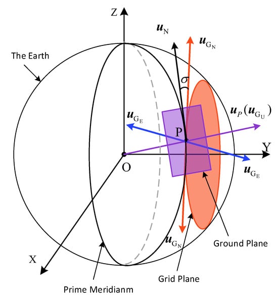
Figure 1.
Definition of the grid coordinate system.

Table 1.
Symbol description in the grid coordinate system.
The directions of some vectors and the values of the parameters are defined as follows:
- : The unit vector points from the center of earth to the point P.
- : The unit vector lies on the intersecting line between the grid plane and the ground plane. Depending on the different definitions of the north direction in the grid frame, it can be defined in two potential (and opposite) directions.
- : The unit vector which is collinear with .
- : A unit vector where , , and conform to the right-hand rule.
- : If is positioned to the east of , then the sign of angle is positive. Otherwise, the sign is negative. The unit is in degrees.
2.2. Discussion on the Definition of the Grid Northward Direction
2.2.1. Definitions of the Existing and Proposed Grid Northward Direction
The northward direction of the grid coordinate is crucial for defining grid angles, calculating grid heading angles, and determining UAV states. However, there is currently no consensus in the academic community regarding its precise definition.
As shown in Figure 2, the northward direction of the grid coordinate is defined on the intersecting line between the grid plane and the local horizontal plane. With P as the origin, two rays pointing towards both sides of the intersection line, namely and , can be defined as the north direction of the grid coordinate system. To determine a more suitable northward direction, there are various definitions of the north direction.
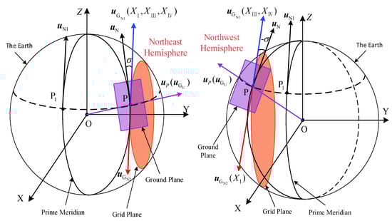
Figure 2.
Definition of the northward direction of the grid coordinate system in the Northeast Hemisphere and Northwest Hemisphere.
Three main definitions and the proposed definition of the grid frame northward direction are introduced as follows:
Definition 1.
(Vector
in Figure 2): The northward direction is parallel to the intersecting line between the grid plane and the ground plane and points to the northeast [12].
Definition 2.
(Vector
in Figure 2): Approximating the polar regions as a flat plane, the northward direction lies on the plane and aligns with the northward direction of the 0° meridian [8]. Since it is an approximate definition, it is unavailable over a large area. Therefore, Definition 2 is neither discussed nor used in this paper.
Definition 3.
(Vector
in Figure 2): The northward direction follows the intersecting line between the grid plane and the ground plane. Starting at the center of the grid coordinate system, it points towards the northeast in the Eastern Hemisphere and towards the northwest in the Western Hemisphere, respectively [13].
However, according to the analysis below, the north direction defined by the three definitions undergoes a significant change at the boundary between the hemispheres. This discontinuous change in the north direction causes a jump in the guidance command. To address this problem, a global applicable definition of the grid north direction is presented as follows:
Definition 4.
(Vector
in Figure 2): Set as the intersecting point of the latitude circle through P and the 0° meridian. Set as the northward direction of the ground plane where is situated. Then, the direction closest to among and is defined as the north direction of the grid coordinate system. Specifically, if the angle between and is less than 90°, is the north direction; otherwise, is the north direction.
2.2.2. Comparison of the Three Definitions near the North Pole
Subsequently, we will summarize the most appropriate definition by comparing the directional continuity of the definitions and their consistency with the grid angle calculation formulas. As shown in Figure 3, for better visual presentation, approximating the polar region as a plane, the center of the plane is the North Pole (N) in the Northern Hemisphere or the South Pole (S) in the Southern Hemisphere, and the plane is partitioned into four regions by four meridians: 0°, 90° E, 180°, and 90° W, whose arrows indicate toward the point N or depart from the point S. In each of the four regions, take a point labeled A, B, C, and D, respectively, with their longitudes , , , (the unit is in degrees) and grid angles , , , . The grid coordinate system has two possible northward directions: , which aligns with the northward direction of the 0° meridian, and , which aligns with the northward direction of the 180° meridian. The notation denotes that the vector refers to in the Northern Hemisphere and refers to in the Southern Hemisphere.
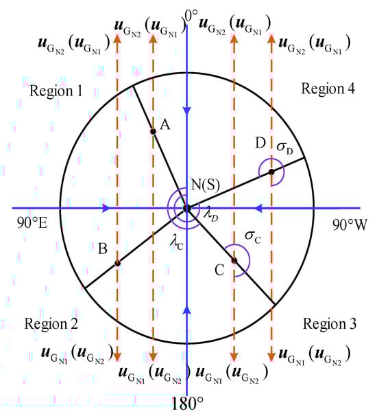
Figure 3.
Definition of the northward direction of the grid frame near the North Pole.
The northward directions under the three definitions in four regions near the North Pole are represented in Table 2, where the red background indicates that the north direction under this definition exhibits discontinuous jumps between different regions.
Table 2.
The directions under three definitions in four regions near the North Pole.
The contiguity of the four definitions around the Northern Hemisphere was analyzed as above, and the consistency of formulas for calculating grid angles and the grid angles under the four definitions were tested.
The calculation of grid angles is given as Equations (1) and (2), and its detailed implementation process can be found in [15], where and L are the longitude and the latitude of the current position.
If the UAV’s position is very close to the North Pole, then and . As a result, Equations (1) and (2) could be simplified as follows:
It can be deduced from Equations (3) and (4) that near the North Pole. As shown in Figure 3, at points C and D, the grid angle equals longitude only if the northward direction of the grid frame and are in the same direction; otherwise, the grid angle is 180° less than the longitudes. Similarly, at A and B, the grid angle equals the longitude only when the northward direction of the grid frame is the same as . As a result, the correct definition of the north direction conforms to Equations (3) and (4) and must be parallel to in the Northern Hemisphere.
The blue background in Table 2 indicates that the defined north direction does not comply with Equations (3) and (4) in the region. As shown in Table 2, both Definition 1 and Definition 4 comply with the constraint in the Northern Hemisphere. Conversely, Definition 1 does not conform to the constraint, and the north direction of Definition 1 will undergo a significant change at the boundary between the Eastern and Western Hemispheres.
2.2.3. Comparison of the Three Definitions near the South Pole
If the UAV is very close to the South Pole, and . As a result, Equations (1) and (2) can be simplified as Equations (5) and (6).
It can be deduced from Equations (5) and (6) that near the South Pole. The directions under the three definitions in four regions near the South Pole are represented in Table 3. Consistent with Section 2.2.3, both directional consistency and formula compliance are annotated in the table.
Table 3.
The directions under three definitions in four regions near the South Pole.
It can be seen from Table 2 and Table 3 that only Definition 4 complies with the constraint in both hemispheres, while the northward direction of Definition 1 undergoes a significant change at the boundary between the Eastern and Western Hemispheres, and the direction of Definition 3 undergoes a significant change at the boundary between the Northern and Southern Hemispheres.
2.3. Globally Applicable Definition of Grid Frame
In conclusion, based on the results of Section 2.2.2, the north direction of Definitions 1 and 3 undergoes a significant change at the boundary between the hemispheres. These significant changes can lead to an abrupt change in the grid azimuth angle and then causes a high-frequency oscillation in the heading commands, which may result in an aviation accident. On the contrary, Definition 4 proposed in this paper is feasible and continuous because it meets the constraints globally and does not cause directional discontinuities. Therefore, the proposed grid north direction can be globally applied, and the subsequent derivations and proofs will adhere to this definition. The proposed definition of the grid frame is described as follows:
Denote point P as the current position of the UAV. The origin of the grid frame is P. The grid plane passes through P and is parallel to the Prime Meridian. Set as the intersecting point of the latitude circle through P and the 0° meridian. Set as the northward direction of the ground plane where is situated. Then, the direction closest to among and is defined as the north direction of the grid coordinate system. Specifically, if the angle between and is less than 90°, is the north direction; otherwise, is the north direction. The upper direction of the grid frame is collinear with the geographic vertical. The east, north, and upper directions of the grid frame conform to the right-hand rule.
3. Calculation of Grid Azimuth Along a Great Ellipse Route
Heading is the crucial guidance information for the guidance algorithm. Since the inverse solution algorithm for the great circle route has been derived, the relationship between the route’s azimuth and the aircraft’s real-time position can be determined [22,23,24,25]. Therefore, the flight management computer (FMC) can use this formula to generate guidance commands to achieve automatic flight. The directional output of grid mechanization is the grid azimuth rather than true azimuth, since the calculation error of the grid heading in polar regions does not diverge; the grid heading is a reliable heading reference in polar regions. However, the grid heading dynamics along a great ellipse route have seldom been researched, resulting in UAVs being deprived of accurate grid heading guidance information for great ellipse route navigation. To address this problem, based on the WGS-84 reference ellipse model and the proposed grid frame definition, the explicit calculation formula of the grid heading angle along the great ellipse route is derived in this section. With the calculation formula for the grid heading, the flight management computer (FMC) can generate the desired grid heading along a great ellipse route. This enables the FMC to plan the course in advance and control the UAV to adjust its heading in time, thus preventing the UAV from veering off the desired course and causing accidents. As a result, the calculation of the grid heading angle significantly enhances the decision-making and risk-avoiding capability of the flight management system (FMS).
3.1. Definition of Great Ellipse Route and Relevant Vectors
The Earth-centered, Earth-fixed (ECEF) system is shown in Figure 4. The origin of the ECEF system is the center of the Earth. The OX axis and OY axis lie on the equatorial plane and point towards the 0° meridian and the 90° E meridian, respectively. The OZ axis is perpendicular to the OX axis and OY axis and conforms to the right-hand rule. The great ellipse route is defined by the departure point and the destination point . The relevant vectors and parameters used in the equation derivation are defined in Table 4.
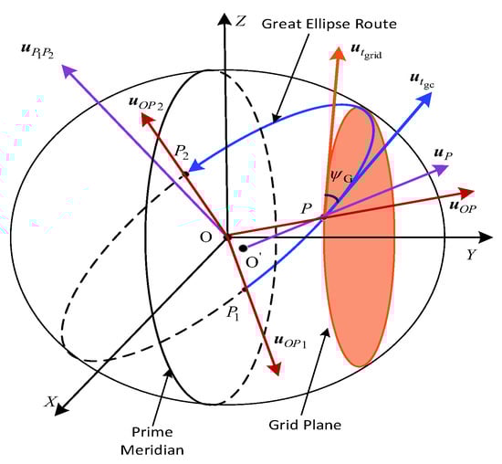
Figure 4.
Schematic diagram of the ECEF coordinate system and some important vectors based on the WGS-84 reference ellipse model.
Table 4.
Symbol description in WGS-84 reference ellipse model.
The directions of some vectors and the values of the parameters are defined as follows:
- : It is a unit vector, and its direction conforms to the right-hand rule relative to the positive direction of the great ellipse route.
- : It is a unit vector tangent to the great ellipse route and points in the forward direction. Additionally, lies along the intersecting line of the great ellipse route and the ground plane at the point P.
- : It is a unit vector parallel to the northward direction of the grid coordinate system on the grid plane.
- : It is the angle between and . It is positive when lies on the right side to from the view above the ground plane; otherwise, it is negative.
3.2. Derivation of the Calculation of the Grid Azimuth Along a Great Ellipse Route Based on the WGS-84 Reference Ellipse Model
This section derives the relationship between the geodetic coordinates (latitude, longitude, and altitude) of a point on the great ellipse route and the grid azimuth of the route at the point. Specifically, the input of the proposed calculation is the geodetic coordinates of the departure point, arrival point, and current point of the route. Its output is the grid azimuth of the great ellipse route at the current point.
The key to deriving the equation lies in establishing the relationship between the grid azimuth and the geodetic coordinates. This section employs key vectors, such as and , as intermediaries. First, these vectors are expressed in terms of geodetic coordinates, and then the relationship between the vector and the grid azimuth is established, thus culminating in the final expression relating the coordinates to the azimuth.
3.2.1. Derivation of the Relationship Between Vectors and Coordinates
The projection of the geographic vertical at the point P in the ECEF coordinate system is given as follows, and the detailed derivation can be found in the literature [16].
The projection of the geocentric vector in the ECEF coordinate system is given as follows, and the detailed derivation can be found in the literature [26].
where (m) is the radius of curvature in the prime vertical, and and e are the oblateness and the first eccentricity of the WGS-84 reference ellipse model, respectively. denotes the length of the semi-major axis of the long axis of the WGS-84 reference ellipse model [26].
Since the normal line to the great ellipse surface is perpendicular to every line on the great ellipse surface, it follows that and . Therefore, can be expressed as
where
To simplify the expression, and are represented by their three-axis components in the ECEF system.
Set the vector as the unit vector in the OY direction of the ECEF coordinate system. Given that (1) lies on the grid plane, (2) the grid plane is parallel to the Prime Meridian, and (3) is perpendicular to the Prime Meridian, it follows that . Because (1) lies on the great ellipse surface and (2) is perpendicular to the great ellipse surface, it follows that .
Since and lie on the ground plane and is perpendicular to the horizontal plane, and can be calculated as follows:
Substituting Equations (11) and (12) into (13) and (14), the specific forms of and can be obtained.
3.2.2. Derivation of the Relationship Between the Vectors and the Grid Azimuth
The grid azimuth is the angle between and . By analyzing the spatial relationship between vectors and and utilizing the formulas for the dot product and scalar triple product, we can express and as follows:
3.2.3. Derivation of the Relationship Between the Coordinates and the Grid Azimuth
The unit vector is subject to the constraint as follows:
Since , Equation (20) can be derived.
The angle difference between and is approximately equal to [16], where is the oblateness of the earth and under the WGS-84 ellipse reference model. In the polar region, and are essentially identical, since . For example, if L = 89.95°, , and if L = 85°, ; therefore, can be neglected in polar regions. Consequently, in the polar region, in Equation (20) can be approximately replaced by
Substituting Equations (20) and (21) into Equations (17) and (18), the specific expression of and can be obtained.
Substituting Equation (7) into (22) and (23), we can obtain
Substituting Equation (9) into Equations (24) and (25), the final expression of under the WGS-84 ellipse model can be derived.
4. A High-Precision Polar Flight Guidance Algorithm
A high-precision flight guidance algorithm is crucial for ensuring the accurate trajectory tracking of UAVs. It plays a role as critical as navigation algorithms (such as GINS) in guaranteeing high-precision and stable operations in polar regions. Based on an analysis of the limitations of conventional flight guidance algorithms in polar regions, this section proposes a precise flight guidance algorithm based on heading prediction and fuzzy decision-making methods. The overall framework of the proposed algorithm is illustrated in Figure 5.
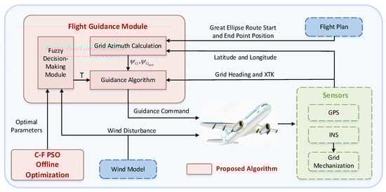
Figure 5.
Flight guidance algorithm scheme.
4.1. Conventional Guidance Algorithm for Great Ellipse Route
Conventional guidance algorithms usually control a UAV to track the great ellipse route in the coordinated turn mode. The guidance law is given as follows:
or
where is the roll command, is XTK, and its detailed implementation process can be found in the literature [22,23,24]. is the differential of cross-track error (XTK). and are the gains.
Since computers cannot calculate pure differentiation, in Equation (29) is replaced by pseudo-differentiation, and its transfer function is given in Equation (30). It bears mentioning that in Equation (30).
Due to the lack of damping terms in Equation (28), the heading of a UAV with this guidance algorithm constantly falls into oscillation in polar regions. The differential signal in Equation (29) enhances the damping of heading control, improving the control stability while the UAV is tracking the great ellipse route, which changes its heading rapidly in polar regions. However, also increases the magnitude of high-frequency sensor noise in polar regions.
To address this problem, in Equation (29) can be replaced by the heading of the UAV. The principle is shown as follows:
As shown in Figure 6, the vector denotes the ground speed of the UAV, is the azimuth angle of the rhumb line, and the current heading of the UAV is . According to Figure 6, it can be deduced that
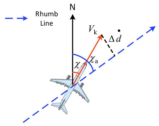
Figure 6.
Schematic diagram of the relationship between different angles in a rhumb line.
Since when UAVs are flying steadily, Equation (31) can be simplified as
Therefore, the guidance law (29) is always replaced by Equation (33) to suppress noise amplification.
As the great ellipse route can be approximated by a group of rhumb lines, the heading-based guidance algorithm (33) is also applicable to the great ellipse route in the low-latitude areas since the azimuth of the great ellipse route changes smoothly and slowly there. However, UAVs equipped with the heading-based flight guidance algorithms cannot track the great ellipse route precisely because the heading of the great ellipse route changes rapidly.
In fact, the key to tracking the great ellipse route accurately is to predict the trend of the heading change and control the plane in advance based on the predicted information. Therefore, after analyzing the difficulties of traditional flight guidance algorithms, a precise flight guidance algorithm based on heading prediction and the fuzzy decision-making method was proposed.
4.2. An Improved Flight Guidance Algorithm for the Great Ellipse Route in Polar Regions
4.2.1. Design of Flight Guidance Algorithm Based on Heading Prediction and Fuzzy Decision-Making Method
To tackle the difficulties of traditional flight guidance algorithms, an improved guidance algorithm is proposed and can be given as follows:
where is the current grid heading that can be obtained by grid mechanization. denotes the desired grid heading at the current UAV position that can be calculated by Equations (26) and (27). is the predicted grid heading at the UAV position T seconds later. , , and are the gains. The expression of the sigmoid function can be given as Equation (35).
Since the predicted grid heading is introduced in this algorithm, the FMS with this algorithm can guide the UAV to change its heading in advance, thereby improving the tracking accuracy of the UAV in polar regions.
The sigmoid functions and are introduced to account for the proportions of the current grid heading error and the predicted grid heading error T seconds later in the control signal. It determines whether correcting the current heading error or controlling the future heading is more important. Since the calculation of the grid heading is based on the premise that the UAV must fly along the great ellipse route precisely, if XTK is excessively large, the prediction will be inaccurate. In this situation, the proportion of the current grid heading should be larger than that of the prediction to avoid worsening the heading and position error caused by inaccurate prediction. The sigmoid functions can account for the proportion dynamically depending on XTK. If XTK is excessively large, the proportion of the current grid heading error approaches 1, while the proportion of the prediction nears 0; therefore, the impact of inaccurate prediction could be avoided. In contrast, if XTK is 0, both of the proportions are 0.5, enabling the UAV to both maintain its current heading and predict its future heading. The tolerance for XTK varies with the flight task requirements; therefore, is introduced to adjust the tolerance for XTK. The value of is determined based on the statistics of flight trials. Suppose the required tolerance of XTK is ; then the basic principle for tuning is shown as follows:
(1) First, roughly determine the boundary of : The proportions ratio should be larger than 10 when to avoid the XTK from exceeding the tolerance and the proportions ratio should be less than 3 when to improve the guidance accuracy in a steady state. Consequently, the upper and lower limits of can be determined.
(2) Second, fine-tune based on trials: Place the vehicle meters away from the great ellipse route at the concave side and then guide the vehicle along the great ellipse route, tuning to minimize the average XTK during the whole flight.
However, if the look-ahead time of prediction, namely T, is set as a fixed value, the guidance accuracy may not be ideal. On the one hand, the specific value of T is tuned by the trial-and-error method, but the process of trial-and-error is inefficient and cannot find the optimal value of T. On the other hand, the guidance algorithm with fixed predictive time lacks the flexibility to respond to varied situations in polar regions. For example, when a UAV encounters a wind disturbance or has deviated from the planned route, the top priority is to keep the UAV flight steady and track the current route rather than predicting. And the prediction accuracy may not be ideal. Therefore, T should be selected as a smaller value in this situation to ensure flight safety. Conversely, when the circumstance is steady, T should be larger to improve the guidance accuracy. As a result, T should be variable and adjusted dynamically depending on the situation. However, the situation is complex and there is no specific relationship between T, XTK, and wind speed; therefore, the adjustment can only rely on human experience. The fuzzy decision-making method mirrors human decision processes. It computes outputs based on abstract, fuzzy input–output relationships rather than precise mathematical ones, making it well suited for solving these problems [27]. The design process of the fuzzy decision system is shown as follows:
(1) Choice of Fuzzy Decision Framework
We choose the Mamdani framework as the fuzzy decision framework. As one of the most classical types of fuzzy decision systems, the Mamdani framework operates with both inputs and outputs as fuzzy sets, typically using IF–THEN rules.
(2) Design of Input Variables and Output Variable
Since the predicted heading is calculated based on the assumption that the UAV is close to the route, the crosswind velocity , which may interfere with future positions, and XTK, which indicates the degree of deviation, are selected as the input variables, with their domains and , respectively. The look-ahead time of prediction, namely T, is the output variable with its domain [0, Ts], where Ts is the setting time of the heading channel of the UAV. The fuzzy subset has 10 members {ZO, PSS, PS, PSB, PMS, PM, PMB, PBS, PB, PBB}.
(3) Design of Membership Function
The Gaussian, triangular, trapezoid, and sigmoid functions are selected to design member functions. The membership function of XTK, crosswind velocity, and look-ahead time T are shown in Figure 7. (1) With respect to the selection of the membership function for T, the decision-making method PBB is risky when the prediction is not precise, so the Gaussian function is selected to avoid extreme decision-making. In order to ensure flight safety, the shape of ZO should be as narrow and sharp as possible, such that the defuzzificated output T can be as low as possible every time the ZO decision is made. Thus, the trapezoidal membership function is selected as the ZO membership function. (2) For XTK, when its value is small, the impact track deviation has on the prediction performance is negligible. Therefore, the Z-shaped membership function (zmf) is selected for the ZO fuzzy set to construct a dead zone. Conversely, when XTK is large, the sigmoid function is selected for the PB fuzzy set. (3) For crosswind, its influence on prediction accuracy is always present regardless of its magnitude. Furthermore, prediction becomes largely ineffective when the crosswind is excessively strong. Hence, a trapezoidal membership function is used for the PB fuzzy set.
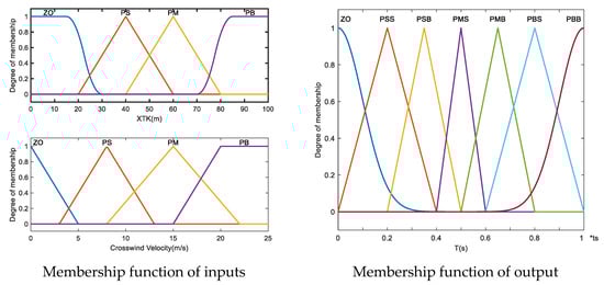
Figure 7.
Membership function of inputs and output.
Given that other situations are approximately symmetrical, to facilitate analysis, the triangular function is selected. We treated the range of each membership function as a parameter to be optimized and used the PSO algorithm for this purpose. It bears mentioning that the domain and range of membership functions are normalized by the linear method while optimizing.
(4) Design of Fuzzy Rules
The fuzzy rule follows basic engineering: The larger the XTK and crosswind velocity, the smaller the look-ahead time of prediction should be. In addition, since flight safety is the top priority, if either XTK or crosswind velocity is PB, T should be ZO to ensure the flight steadiness first. Therefore, the specific fuzzy rule is shown in Table 5.
Table 5.
Fuzzy rules of T.
(5) Design of the Defuzzification Method
The centroid method is selected as the defuzzification method and expressed in Equation (36).
where z is the output of defuzzification and is the membership function of z.
4.2.2. Parameter Tuning for Fuzzy Decision-Making Module Based on Improved Particle Swarm Optimization (PSO) Algorithm
Although some parameters in the fuzzy decision-making module, such as the number and form of membership functions, can be set empirically, other parameters, such as the center positions and domains of membership functions, are more complex to adjust, often yielding suboptimal results. Thus, an improved concave function fitness-based particle swarm optimization (C-F PSO) algorithm is introduced to optimize the center positions and domains of membership functions.
The complete PSO algorithm comprises encoding, fitness function construction, and update strategies. A detailed introduction to the algorithm is provided in [22,28]. In this study, variable wind disturbances are introduced in each simulation and the integral of the absolute value of XTK is selected as the fitness function in Equation (37).
This section focuses specifically on update strategies, and the standard particle update formulas are summarized below. The corresponding parameters are defined in Table 6.
where the inertial weight is a crucial parameter in the particle updating process, characterizing the particle’s ability to sustain its motion and expand its search. To balance rapid search in the early stage with convergence in the later stage, a linear adaptive adjustment strategy for is commonly used:
Table 6.
Symbol description in PSO algorithm.
As the number of iterations increases, the inertia weight decreases linearly. This allows the PSO algorithm to maintain strong global exploration initially and shift to accurate local convergence in later stages.
However, unlike optimization for fixed operating condition problems, variable wind disturbances are introduced in each simulation to enhance the robustness of the fuzzy decision-making module against different wind disturbance situations. In this varying-condition optimization process where the situation differs per iteration, an inertia weight (adjusted by Equation (38)) that is too small in the later stages would cause the PSO algorithm to effectively ignore some wind disturbance scenarios. This can easily lead to convergence to a local optimum and compromise robustness against diverse wind conditions. To address this issue, a dynamic adjustment method for the inertia weight based on a concave function model is introduced (C-F adjustment strategy) to balance global exploration and local convergence capabilities.
where b is a control factor used to adjust the attenuation rate. Assuming , the inertia weight curves of the linear adaptive adjustment (Equation (38)) and concave function adaptive adjustment (Equation (39)) are shown in Figure 8.
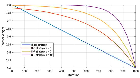
Figure 8.
Inertia weight curves of linear adaptive adjustment and concave function adaptive adjustment.
Compared to the linear adaptive strategy, the proposed C-F approach enables more effective exploration of the search space in early iterations. This configuration helps particles quickly locate better solutions while avoiding convergence to local optima. As the iterations progress, the inertia weight rapidly decreases, prompting particles to focus more on their best positions while maintaining their search and adaptation capabilities for new scenarios. The detailed flowchart of the progress of C-F PSO is shown in Figure 9.
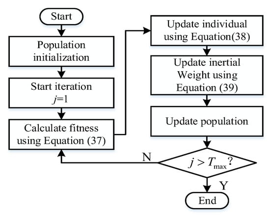
Figure 9.
Schematic diagram of the C-F PSO process.
5. Experimental Design and Result Analysis
5.1. Simulation Conditions
To assess the proposed algorithms, some simulations are operated under the following conditions:
(1) Choice of segment: ① A great ellipse route from London Heathrow Airport to the Anadyr Airport in Chukchi Autonomous Region, Russia, is selected. The route passes through the polar region and spans the Eastern Hemisphere, making it significantly shorter than non-polar routes and thus of considerable commercial value. To reduce simulation time and computational load, only the segment of the route with a latitude above 89.5° is used for numerical simulation. The complete great ellipse route and its high-latitude segment are shown in Figure 10. ② For rigorous validation, a special great ellipse route passing directly through the North Pole from to is also simulated.
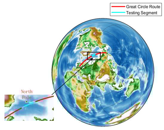
Figure 10.
Schematic diagram of the great ellipse route.
(2) Settings of UAV:
The initial position of the UAV is always set to the same as the start point of the great ellipse route. The initial speed is set to constant values of 150 m/s. The main parameters of the UAV are shown in Table 7.
Table 7.
Key parameters of drone.
(3) Settings for disturbance
To evaluate the robustness of the proposed guidance algorithm, 1000 stochastic simulations are conducted via the Monte Carlo method under sensor noise and wind disturbance. The drift of the gyro is 0.01°/h, and the random walk is 0.002°/√h. The drift of the accelerometer is 50 ug, and the random walk is . The wind field settings include constant winds of 5 m/s, 10 m/s, 15 m/s, and 20 m/s, as well as atmospheric turbulence and wind shear (the model is sourced from document AC120-41 [29]).
(4) Settings of guidance laws
The following four guidance laws are selected to guide the UAV to track the two great ellipse routes. Note that the parameters of the four guidance laws remain consistent in this simulation.
Guidance Law I: Only control XTK:
Guidance Law II: Control XTK and its differential:
Guidance Law III: Control XTK and the deviation of the azimuth:
Guidance Law IV: The guidance algorithm proposed in this paper:
The relationship between and the proportions ratio is shown in Figure 11. In this simulation, the gain is 50. If XTK is 50 m, then . The proportions ratio between the current grid heading angle deviation and the future grid heading angle deviation is approximately 3:1. If XTK is 100 m, then . The weight proportion between the current grid heading angle deviation and the future grid heading angle deviation is approximately 7:1. is chosen to be 100 m and is chosen to be 20 m/s.
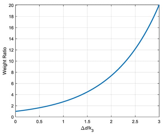
Figure 11.
The relationship between and the proportions ratio.
(5) Evaluation metric
According to RTCA-DO-236C (Minimum Aviation System Performance Standards) [30], XTK and the grid heading deviation are selected as metrics to evaluate the guidance performance.
(6) Experimental process
The experimental process is demonstrated in Figure 12.
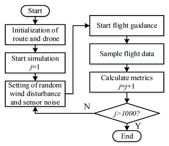
Figure 12.
The experimental process.
(7) Data collection
During the flight, the aircraft’s position, grid heading angle, lead time output from the fuzzy decision-making module, and crosswind velocity are collected for metric calculation.
5.2. Results and Analysis
Three sets of simulations are conducted as follows: (1) tuning of the fuzzy decision-making module, (2) evaluation of the flight guidance algorithm’s performance along common great ellipse routes, and (3) evaluation of the algorithm’s performance along special great ellipse routes.
5.2.1. Fuzzy Decision-Making Module Parameter-Tuning Simulation
To evaluate the effectiveness of the proposed C-F PSO in optimizing the fuzzy-decision-based variable prediction time guidance algorithm in Equation (40), a comparative simulation was performed including the following three cases: (1) a guidance algorithm with the fixed prediction time (), (2) a guidance algorithm with fuzzy-decision-based variable prediction time tuned by PSO, and (3) a guidance algorithm with fuzzy-decision-based variable prediction time tuned by C-F PSO. The parameter tuning and simulation results are shown in Figure 13, Figure 14 and Figure 15.
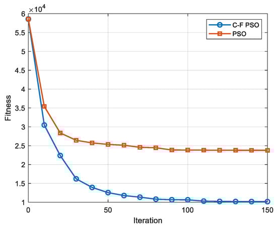
Figure 13.
Parameter tuning results of C-F PSO and PSO.
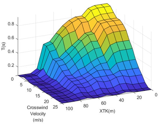
Figure 14.
Fuzzy decision rules tuned by C-F PSO.
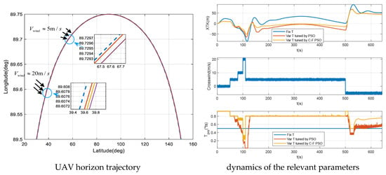
Figure 15.
UAV horizontal trajectory and relevant parameters in three cases.
As shown in Figure 13, in the context of optimizing for variable wind fields, the C-F PSO algorithm can rapidly tune parameters initially while still adapting to new wind conditions later, thus avoiding local optima. The simulation result in Figure 15 illustrates that the C-F-tuned, fuzzy-decision-based variable prediction time guidance algorithm achieves the best guidance performance under wind disturbance, with an XTK value of less than 50 m and the fastest convergence rate.
Figure 14 represents the fuzzy decision rules tuned by C-F PSO, i.e., the relationship between the input (crosswind speed and XKT) and output (look-ahead time) of the fuzzy decision-making module. It is in accordance with the fundamental principle that look-ahead time decreases with crosswind speed and XTK.
The superiority of variable prediction time is now analyzed from the perspectives of the operational mechanism and physical principles.
In the right-side diagram in Figure 15, from 0 s to 50 s, since the velocity of the crosswind is 0 m/s, a maximum look-ahead time is generated to achieve a higher guidance accuracy. From 100 s to 110 s, since the UAV encounters severe wind shear, a minimal look-ahead time is generated to ensure the stabilization of the UAV and correct the lateral deviation first rather than predicting. As a result, the UAV’s XTK is adjusted back to 0 faster. The wind disturbance is weak from 110 s to 500 s, so T becomes larger, and XTK is almost 0 m.
The flight situation from 100 s to 110 s is shown in Figure 16. As shown in Figure 16, predicted points 1 and 2 are two points calculated under two typical situations. Predicted point 1 corresponds to a shorter look-ahead time (calculated by the fuzzy decision-making method) so the point is closer to the plane. In contrast, predicted point 2 indicates a longer look-ahead time (the fixed look-ahead time T) and the point being farther away from the plane. and are the predicted velocities at points 1 and 2, respectively. For the simplicity of the expression, symbol simultaneously denotes and in the following discussion.
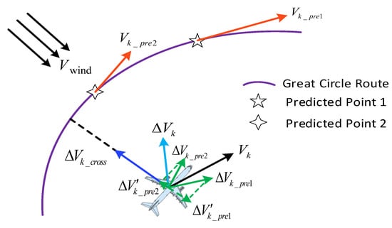
Figure 16.
Flight situation from 100 s to 110.
From 100 s to 110 s, the UAV significantly deviated from the great ellipse route because of the wind shear. At the same time, the increment of the track velocity vector, namely , was generated by the control effect of the guidance law. can be divided into two parts, namely , which is generated by the term in the guidance algorithm to correct the lateral deviation, and , which is generated by the term to follow the predicted track velocity vector . denotes the component of which is parallel to . As shown in Figure 16, if the look-ahead time is longer, namely predicted point 1, is opposite to , therefore preventing the UAV from approaching the planned route. On the contrary, if the predicted time is shorter, namely predicted point 1, and are in the same direction, thereby hastening heading adjustment. Consequently, the variable T generated by the proposed fuzzy-decision method is beneficial for the guidance algorithm to ensure lateral stability and accuracy under wind disturbance.
5.2.2. Guiding the UAV Along the General Great Ellipse Route
To evaluate the performance of the proposed heading prediction-based guidance law, it is compared against conventional guidance laws (Equations (37)–(39)). The influence of wind disturbance and sensor noise are considered, and the wind model is constructed based on the Kaimal spectrum [31]. The dynamics in latitude, longitude, and desired heading are shown in Figure 17. It can be seen that the desired heading changes rapidly on this great ellipse route.
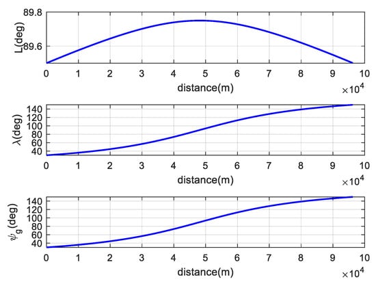
Figure 17.
Dynamics in latitude, longitude, and desired azimuth of the great ellipse route with distance.
The simulation result of guidance law I is shown in Figure 18. Since the UAV guided by guidance law I lacks the damping in the heading channel, the heading of the UAV tends to oscillate. As a result, guidance law I is not suitable in the polar region.
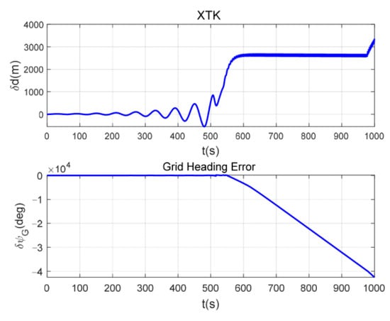
Figure 18.
Dynamics in XTK and grid heading error of guidance law I with time.
The simulation results of the other three guidance laws are shown in Figure 19 and Figure 20, and the statistical data for XTK and grid heading error of 1000 stochastic simulations are presented in histograms, as shown in Figure 21, Figure 22 and Figure 23 and Table 8.
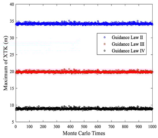
Figure 19.
Maximum XTK of three algorithms in each stochastic simulation.
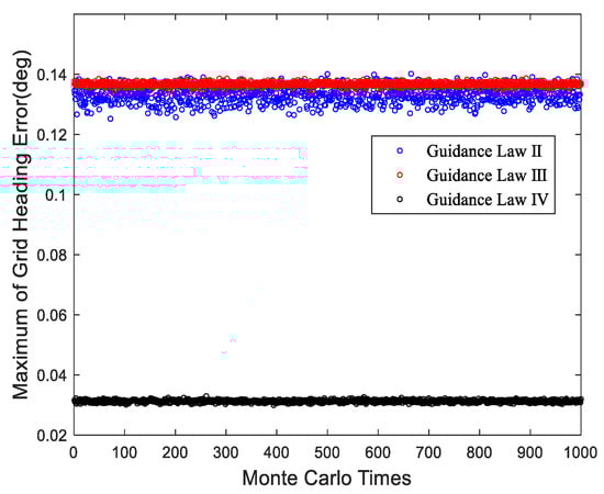
Figure 20.
Maximum grid heading error of three guidance laws in each stochastic simulation.
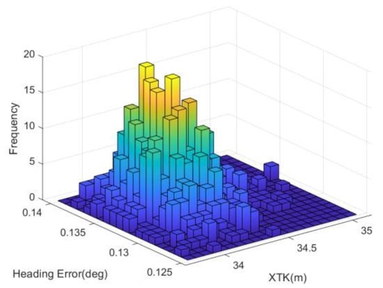
Figure 21.
Statistical data of guidance law II.
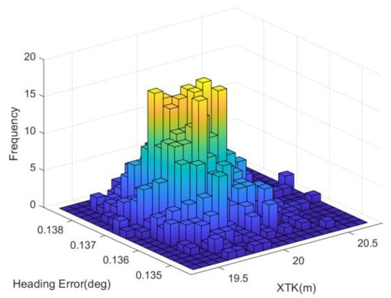
Figure 22.
Statistical data of guidance law III.
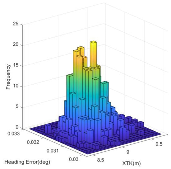
Figure 23.
Statistical data of guidance law IV.
Table 8.
Statistical data of three guidance laws.
As seen in Figure 18, Figure 19 and Figure 20, the frequency histogram of the proposed algorithm is more acute and focused than the other algorithms, which means the proposed algorithm is steadier under the sensor noise disturbance.
A comparison between the proposed guidance law and traditional guidance laws is shown in Table 9. As indicated in Table 9, the heading accuracy under the proposed algorithm is five times that of the traditional method, while its variance is 2.6% of the traditional method. Moreover, the position accuracy under the proposed algorithm is three times that of the traditional algorithms. These results demonstrate that the proposed guidance algorithm can guide the UAV to fly along the planned great ellipse route in polar regions with high precision and strong robustness.
Table 9.
Comparison between the proposed guidance law and traditional guidance law.
5.2.3. Guiding the UAV Along the Great Ellipse Route Passing Through the North Pole
To ensure comprehensive simulation verification, a special route passing through the North Pole was employed for simulation, while the remaining conditions remained consistent with those described in Section 5.2.2. The maximum XTK of the UAV guided by three guidance laws in each stochastic simulation is shown in Figure 24.
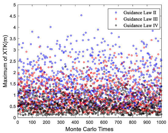
Figure 24.
Maximum XTK of three guidance laws in each stochastic simulation.
It can be seen from the results that the XTK under the three guidance laws is not significantly different. That is because the great ellipse route passing through the North Pole must be a meridian, with the heading remaining constant, thus allowing the UAV to track the route easily.
6. Conclusions and Future Work
In this paper, a globally applicable definition of grid frame was proposed. On this basis, a precise flight guidance algorithm based on heading prediction and the fuzzy decision-making method was proposed. Herein, a grid azimuth formula on the great ellipse route based on the WGS-84 ellipse model was derived to achieve accurate heading estimation and prediction. The predicted grid heading generated by the formula is applied in the guidance algorithm to cope with the rapid changes in heading, therefore enabling the UAV to predict and adjust the heading in advance, increasing the flight guidance accuracy. In order to ensure prediction accuracy under emergencies, such as wind shear and sensor fault, a fuzzy decision-making method is applied to adjust the look-ahead time, and an improved PSO algorithm is adapted to tune the parameters. To verify the effectiveness of the proposed algorithm, a flight guidance simulation based on a typical great ellipse route in the polar region was conducted, and it can be seen from the results that the proposed algorithm demonstrates 3–4 times higher accuracy in heading and position guidance compared to conventional algorithms.
While this article has made contributions to the field of polar flight guidance, there are still areas for improvement and further research. Future work will focus on testing and performance evaluation of the proposed algorithms in real-world scenarios.
Author Contributions
Conceptualization, J.C. and G.L.; methodology, J.C.; software, J.C. and J.M.; validation, J.C., S.Z. and G.L.; formal analysis, J.C.; investigation, J.C., S.Z. and G.L.; resources, G.L. and J.M.; data curation, J.C.; writing—original draft preparation, J.C., Y.H. and G.L.; writing—review and editing, J.C., G.L., S.Z. and J.M.; visualization, J.C.; supervision, J.C., G.L., S.Z. and J.M. All authors have read and agreed to the published version of the manuscript.
Funding
This work is supported by the Aeronautical Science Foundation of China (No. 20240007053005).
Data Availability Statement
The raw data supporting the conclusions of this article will be made available by the authors upon request.
Conflicts of Interest
The authors declare that they have no known competing financial interests or personal relationships that could have appeared to influence the work reported in this paper.
References
- Cui, W.T.; Ben, Y.Y.; Zhang, H.X. A Review of Polar Marine Navigation Schemes. In Proceedings of the IEEE Symposium on Position Location and Navigation, Portland, OR, USA, 20–23 April 2020; pp. 851–855. [Google Scholar] [CrossRef]
- Sun, J.L.; Ma, S.H.; Wang, J.; Yang, J.; Liu, M. Reconciliation Problem in Polar Integrated Navigation Considering Coordinate Frame Transformation. IEEE Trans. Veh. Technol. 2020, 69, 10375–10379. [Google Scholar] [CrossRef]
- Jiang, P.F.; Geng, X.S.; Pan, G.W.; Li, B.; Ning, Z.W.; Guo, Y.; Wei, H.W. GNSS Anti-Interference Technologies for Unmanned Systems: A Brief Review. Drones 2025, 9, 349. [Google Scholar] [CrossRef]
- Qin, F.J.; Chang, L.B.; Li, A. Improved Transversal Polar Navigation Mechanism for Strapdown INS using Ellipsoidal Earth Model. J. Navig. 2018, 71, 1460–1476. [Google Scholar] [CrossRef]
- Li, J.; Gao, J.; Liang, Z.; Zhang, Y. Analysis of Polar Region Navigation Algorithm of Laser Gyro Single-axis Rotation Modulation Inertial Navigation. J. Phys. Conf. Ser. 2022, 2183, 012030. [Google Scholar] [CrossRef]
- Yan, Z.P.; Wang, L.; Zhang, W.; Zhou, J.J.; Wang, M. Polar Grid Navigation Algorithm for Unmanned Underwater Vehicles. Sensors 2017, 17, 1599. [Google Scholar] [CrossRef] [PubMed]
- Lin, X.X.; Bian, H.W.; Wang, R.Y.; Ma, H. Analysis of Navigation Performance of Initial Error based on INS Transverse Coordinate Method in Polar Region. In Proceedings of the IEEE Csaa Guidance, Navigation and Control Conference (Cgncc), Xiamen, China, 10–12 August 2018; pp. 1–6. [Google Scholar]
- Huang, W.Q.; Fang, T.; Luo, L.; Zhao, L.; Che, F.Z. A Damping Grid Strapdown Inertial Navigation System Based on a Kalman Filter for Ships in Polar Regions. Sensors 2017, 17, 1551. [Google Scholar] [CrossRef] [PubMed]
- Cheng, Y.; Zhou, Q. Test Validation of Indirect Grid Inertial Navigation Mechanization. In Proceedings of the 6th Conference on Signal and Information Processing, Networking and Computers, ICSINC, Guiyang, China, 13–16 August 2019; pp. 409–419. [Google Scholar]
- Song, L.J.; Yang, G.Q.; Zhao, W.L.; Ding, Y.J.; Wu, F.; He, X. The Inertial Integrated Navigation Algorithms in the Polar Region. Math. Probl. Eng. 2020, 2020, 5895847. [Google Scholar] [CrossRef]
- Song, L.J.; Zhao, W.L.; Cheng, Y.X.; Chen, X.Z. Based on Grid Reference Frame for SINS/CNS Integrated Navigation System in the Polar Regions. Complexity 2019, 2019, 2164053. [Google Scholar] [CrossRef]
- Ben, Y.Y.; Cui, W.T.; Li, Q. An Improved Damping Method for Grid Inertial Navigation System in Polar Region. IEEE Trans. Instrum. Meas. 2022, 71, 8505713. [Google Scholar] [CrossRef]
- Fang, T.; Huang, W.Q.; Lynch, A.F.; Wang, Z.Y. Non-damping system reset algorithm for shipborne grid strap-down inertial navigation systems. Meas. Sci. Technol. 2020, 31, 055104. [Google Scholar] [CrossRef]
- Qiu, Z.Y.; Lv, J.N.; Lin, D.F.; Yu, Y.A.; Sun, Z.W.; Zheng, Z.X. A Lidar-Inertial Navigation System for UAVs in GNSS-Denied Environment with Spatial Grid Structures. Appl. Sci. 2023, 13, 414. [Google Scholar] [CrossRef]
- Zhou, Q.; Qin, Y.; Fu, Q.; Yue, Y. Grid mechanization in inertial navigation systems for transpolar aircraft. J. Northwest. Polytech. Univ. 2013, 31, 210–217. [Google Scholar]
- Braasch, M. Fundamentals of Inertial Navigation Systems and Aiding; IET Digital Library; SciTech: London, UK, 2022. [Google Scholar]
- Song, L.J.; Duan, Z.X.; He, B.; Li, Z. Research on SINS/GPS integrated navigation system based on grid reference frame in the polar region. Adv. Mech. Eng. 2017, 9, 1687814017727475. [Google Scholar] [CrossRef]
- Zhao, B.; Zeng, Q.H.; Liu, J.Y.; Gao, C.L.; Zhao, T.Y. A new polar alignment algorithm based on the Huber estimation filter with the aid of BeiDou Navigation Satellite System. Int. J. Distrib. Sens. Netw. 2021, 17, 15501477211004115. [Google Scholar] [CrossRef]
- Fu, Q.W.; Zhou, Q.; Yan, G.M.; Li, S.H.; Wu, F. Unified All-Earth Navigation Mechanization and Virtual Polar Region Technology. IEEE Trans. Instrum. Meas. 2021, 70, 8501211. [Google Scholar] [CrossRef]
- Guo, Z.Q.; Wang, J.H.; Zheng, X.; Zhou, Y.H.; Zhang, J.Q. A Visual Guidance and Control Method for Autonomous Landing of a Quadrotor UAV on a Small USV. Drones 2025, 9, 364. [Google Scholar] [CrossRef]
- Jiao, C.C.; Liu, Z.C.; Hou, J.X. Intelligent Optimization of Waypoints on the Great Ellipse Routes for Arctic Navigation and Segmental Safety Assessment. J. Mar. Sci. Eng. 2025, 13, 1543. [Google Scholar] [CrossRef]
- Yang, L.; Zhai, S.B.; Li, G.W.; Hou, M.S.; Jia, Q.L. Generation of Guidance Commands for Civil Aircraft to Execute RNP AR Approach Procedure at High Plateau. Aerospace 2023, 10, 396. [Google Scholar] [CrossRef]
- Zhai, S.B.; Li, G.W.; Jia, Q.L.; Li, Z.X.; Cai, W.J. Design of Guidance Law for Automatic Landing Meeting the CAT III Standard. In The Proceedings of the 2021 Asia-Pacific International Symposium on Aerospace Technology (APISAT 2021), Volume 2; Lecture Notes in Electrical Engineering Volume 913; Springer: Singapore, 2023; pp. 437–451. [Google Scholar] [CrossRef]
- Zhai, S.B.; Li, G.W.; Cheng, J.M.; Hou, M.S. GBAS-based high-precision automatic landing guidance for civil aircraft using improved active disturbance rejection control. Results Eng. 2025, 27, 105716. [Google Scholar] [CrossRef]
- Li, G. Civil Airliner Flight Guidance Technology for Four-Dimensional Trajectory-Based Operation; Springer Nature: Singapore, 2024. [Google Scholar]
- Wang, C.Y.; Zhang, J.R.; Wang, J.N.; Wu, Y.D. Confidence-Based Fusion of AC-LSTM and Kalman Filter for Accurate Space Target Trajectory Prediction. Aerospace 2025, 12, 347. [Google Scholar] [CrossRef]
- Liu, Y.D.; Ding, D.L.; Tan, M.L.; Luo, Y.Q.; Li, N.; Zhou, H. Tactical Coordination-Based Decision Making for Unmanned Combat Aerial Vehicles Maneuvering in Within-Visual-Range Air Combat. Aerospace 2025, 12, 193. [Google Scholar] [CrossRef]
- Demir, H.G. Grey Wolf Optimization- and Particle Swarm Optimization-Based PD/I Controllers and DC/DC Buck Converters Designed for PEM Fuel Cell-Powered Quadrotor. Drones 2025, 9, 330. [Google Scholar] [CrossRef]
- AC 120-41, Criteria for Operational Approval of Airborne Wind Shear Alerting and Flight Guidance; Federal Aviation Administration: Washington, DC, USA, 1983.
- RTCA DO-236B; Minimum Aviation System Performance Standards: Required Navigation Performance for Area Navigation. Radio Technical Commission for Aeronautics: Washington, DC, USA, 2003.
- Kaimal, J.C.; Izumi, Y.; Wyngaard, J.C.; Cote, R. Spectral Characteristics of Surface-Layer Turbulence. Q. J. Roy. Meteor. Soc. 1972, 98, 563–589. [Google Scholar] [CrossRef]
Disclaimer/Publisher’s Note: The statements, opinions and data contained in all publications are solely those of the individual author(s) and contributor(s) and not of MDPI and/or the editor(s). MDPI and/or the editor(s) disclaim responsibility for any injury to people or property resulting from any ideas, methods, instructions or products referred to in the content. |
© 2025 by the authors. Licensee MDPI, Basel, Switzerland. This article is an open access article distributed under the terms and conditions of the Creative Commons Attribution (CC BY) license (https://creativecommons.org/licenses/by/4.0/).