Disturbance-Observer-Based Fixed-Time Backstepping Control for Quadrotors with Input Saturation and Actuator Failure

Abstract

This paper investigates the fixed-time tracking control problem of an unmanned aerial vehicle (UAV) considering the disturbance, input saturation, and actuator failure. According to the hierarchical control principle, the UAV dynamics are decomposed into a translational and rotational loop to accommodate the controller design. A novel nonsingular fixed-time backstepping controller based on switching variables is proposed to achieve fast convergence of system tracking errors within a fixed time. To overcome the effect of the disturbance and the actuator failure, two fixed-time disturbance observers are designed in two loops, respectively. By integrating the fixed-time auxiliary variables into the dynamic controllers, the problem of input saturation can be addressed. In addition, the tracking errors of the closed-loop system converge to the neighborhood of the origin in a fixed time. Finally, sufficient simulation results verify the validity of the proposed control framework for the UAV.

1. Introduction

In recent years, unmanned aerial vehicles (UAVs) have garnered significant attention across both military and civilian sectors. These versatile devices offer innovative solutions to a variety of applications, including aerial photography, firefighting, search and rescue operations, transportation, even aerial refueling, etc. [1,2,3]. Among the diverse range of UAVs, quadcopter UAVs (QUAVs) have emerged as the most popular choice due to their simplicity and convenience in executing complex tasks. As quadcopters become increasingly integrated into industrial production and daily life, there is a growing demand for enhanced control performance, such as effectively mitigating disturbances and managing actuator failures.

Several classic control strategies have been extensively explored for QUAVs, including proportional–integral–derivative (PID) control [4] and linear quadratic regulator (LQR) control [5]. The sliding mode control (SMC) method, known for its ease of implementation, strong robustness, and fast response, has been applied to control UAVs in the presence of external disturbances [6]. Nonsingular fast terminal SMC has been proposed to achieve finite-time tracking and enhance system robustness [7,8], while a cleverly designed finite-time robust controller was introduced for uncertain time-delay systems [9].

The backstepping algorithm is one of the most popular and effective nonlinear control methods in strict feedback systems and has been successively applied to the QUAVs in [10,11]. However, traditional backstepping control suffers from the “complexity explosion” problem because the repeated differentiation of virtual control laws leads to a dramatic increase in the complexity of the controller. To address this issue, command-filtered backstepping [12] and dynamic surface control (DSC) [13] have been proposed. To enhance the robustness of UAV control, an adaptive backstepping controller has been adopted to effectively suppress disturbances [14,15], and a disturbance observer has been introduced to mitigate external disturbances [16]. To address actuator errors, Wang et al. [17] employed an extended state observer, achieving fault-tolerant control and enabling robust trajectory tracking of UAVs within a finite time frame.

Despite these advancements, the aforementioned methods can only ensure the finite-time stability of the filter errors, meaning the convergence time is theoretically dependent on initial conditions. To eliminate this dependency, the concept of fixed-time control was recently introduced [18]. Unlike finite-time stability, fixed-time control ensures that convergence time is bounded by a constant, regardless of initial conditions, making it an attractive feature for controller design. Studies have developed a modified nonsingular terminal sliding mode surface to achieve fixed-time control for second-order nonlinear systems and multi-agent systems [19]. Using a similar approach, fixed-time position control for UAVs is accomplished by analyzing each channel in [20]. To achieve fixed-time disturbance suppression, the design of a fixed-time disturbance observer (FTDO) for linear systems under measurement noise is discussed in [21]. In [22], a fixed-time differentiator was developed to ensure the tracking performance of hypersonic vehicles. In [23], a nonlinear FTDO was studied to estimate target acceleration.

However, research on fixed-time disturbance rejection and motion control of UAV tracking remains insufficient. The introduction of fixed-time controllers can easily lead to severe chattering in the system, which is unacceptable in practical applications. Additionally, in fixed-time backstepping control, the derivative of the virtual control can exhibit singularities, potentially causing controller failure or even system divergence. Furthermore, the aforementioned studies on fixed-time control do not take into account the input saturation characteristics of the system, a common and critical factor in the actual control of UAVs.

To address the aforementioned issues, this paper proposes a novel nonsingular fixed-time backstepping (NFTBS) control framework based on a fixed-time disturbance observer for QUAV trajectory tracking in the presence of input saturation and actuator failure. Compared with the previous works, the designed control algorithm provides the following attractive contributions:

(1)

Unlike some traditional backstepping controllers proposed in [14,15,16], a fixed-time disturbance-observer-based NFTBS (FTDOB-NFTBS) control framework is developed, which combines the FTDO and the auxiliary variable to eliminate the adverse effects of the external disturbance, actuator failure, and input saturation. The fixed-time stability of the closed-loop system can be guaranteed.

(2)

In contrast to previous results proposed in [24,25], the proposed NFTBS not only stabilizes the system within a fixed time but also guarantees a rapid optimal convergence rate both at a distance from and in close proximity to the reference trajectories.

(3)

Unlike some earlier proposed fixed-time backstepping controllers shown in [25,26], the design of continuous control input signals, along with the implementation of a fixed-time tracking differentiator (TD), effectively addresses the issues of singularity, chattering, and differential explosion that are commonly encountered in fixed-time backstepping control.

The remaining sections of this article are structured as follows: Section 2 presents preliminaries and problem formation. Section 3 details the controller design and provides the stability analysis. Simulation results and discussions are arranged in Section 4. Finally, Section 5 gives conclusive statements.

Notations: In this article, $\mathrm{diag}(·)$ denotes the diagonal matrix. ∘ represents the Hadamard product operator. $C_{(·)}$, $S_{(·)}$, and $T_{(·)}$ correspond to $sin(·)$, $cos(·)$, and $tan(·)$. $|·|$ and $\parallel ·\parallel$ indicate the 1-norm and 2-norm of a vector or variable, respectively. $\mathrm{sign}(·)$ is the signum function. ${⌊·⌉}^{\alpha }={|·|}^{\alpha }\circ \mathrm{sign}(·)$.

2. Preliminaries and Problem Formulation

2.1. System Modeling and Preliminaries

The UAV model is depicted in Figure 1, which includes a rigid cross frame and four rotors. For ease of describing the coordination configuration, the body-fixed frame is represented by ${\mathcal{S}}_B=\left\{O_B{X}_B{Y}_B{Z}_B\right\}$, and the inertia frame is represented by ${\mathcal{S}}_O\{=O_E{X}_E{Y}_E{Z}_E\}$.

Figure 1. Construction and frame of the UAV.

Referring to reference [27], the dynamic model of the UAV can be described as

$$\begin{array}{c}\hfill \begin{array}{cc}\hfill \ddot{\mathit{\eta }}& =\mathit{A}\left(\mathit{\rho }\right){\displaystyle \frac{E_{\eta }\mathrm{sat}\left(u_f\right)}{m}}-{\displaystyle \frac{k_t}{m}}\dot{\mathit{\eta }}-\mathit{g}+{\displaystyle \frac{{\mathit{d}}_{\eta }}{m}},\hfill \\ \hfill \mathit{J}\dot{\mathit{\omega }}& =-k_r\mathit{\omega }-\mathit{\omega }\times \left(\mathit{J}\mathit{\omega }\right)+{\mathit{d}}_{\rho }+{\mathit{E}}_{\rho }\mathrm{sat}\left(\mathit{\tau }\right),\hfill \\ \hfill \dot{\mathit{\rho }}& =\mathit{W}\left(\mathit{\rho }\right)\mathit{\omega },\hfill \end{array}\end{array}$$

(1)

where $\mathit{\eta }={[x,y,z]}^{\top }$, $k_t\in \mathbb{R}$, $u_f\in \mathbb{R}$, and m, respectively, represent the position, drag coefficient of the translational loop, desired thrustm and mass of the UAV. $\mathit{g}={[0,0,g]}^{\top }$ is the gravity vector. $\mathit{\rho }={[\varphi ,\theta ,\psi ]}^{\top }$ with $\varphi ,\theta ,\psi$, respectively, being the roll, pitch, and yaw angles in ${\mathcal{S}}_O$. $\mathit{\omega }={[p,q,r]}^{\top }$ is the angular velocity along three axes in ${\mathcal{S}}_B$. x, y, z, and $\psi$ are the outputs of the system that need to be controlled. $\mathit{J}\in {\mathbb{R}}^{3\times 3}$, $k_r\in \mathbb{R}$ and $\mathit{\tau }={[{\tau }_1,{\tau }_2,{\tau }_3]}^{\top }$, respectively, denote the inertia tensor matrix, the drag coefficient of the rotational loop, and the desired torque of the UAV. ${\mathit{d}}_{\eta }={[d_x,d_y,d_z]}^{\top }$ and ${\mathit{d}}_{\rho }={[d_p,d_q,d_r]}^{\top }$ denote the disturbances; $\mathrm{sat}\left(u_f\right)$ and $\mathbf{s}\mathbf{a}\mathbf{t}\left(\tau \right)={[\mathrm{sat}\left({\tau }_1\right),\mathrm{sat}\left({\tau }_2\right),\mathrm{sat}\left({\tau }_3\right)]}^{\top }$, respectively, denote the nonlinear saturation characteristics of $u_f$ and $\mathit{\tau }$. As described in [28],

$$\begin{array}{cc}\hfill \mathrm{sat}\left(u_f\right)& =\mathrm{sign}\left(u_f\right) \mathrm{m}\mathrm{i}\mathrm{n}\{|u_f|,{\overline{u}}_f\},\hfill \\ \hfill \mathrm{sat}\left({\tau }_i\right)& =\mathrm{sign}\left({\tau }_i\right) \mathrm{m}\mathrm{i}\mathrm{n}\{|{\tau }_i|,{\overline{\tau }}_i\},\hfill \end{array}$$

where $i=1,2,3$, ${\overline{u}}_f$ and ${\overline{\tau }}_i$ are the upper bounds of the actuators. $E_{\eta }$ and ${\mathit{E}}_{\rho }=\mathrm{diag}(E_1,E_2,E_3)$ denote actuator failure indicators for $u_f$ and $\mathit{\tau }$. For $j=1,2,3,\eta$, $E_j=1$ means that the actuator works normally, and $E_j\in (0,1)$ indicates that the j-th actuator has partially lost effectiveness but still works. $\mathit{A}\left(\mathit{\rho }\right)=\left[\begin{array}{c}{C}_{\varphi }{C}_{\psi }{S}_{\theta }+S_{\varphi }{S}_{\psi }\\ C_{\varphi }{S}_{\psi }{S}_{\theta }-S_{\varphi }{C}_{\psi }\\ C_{\theta }{C}_{\varphi }\end{array}\right]$ is the rotation vector, and $\mathit{W}\triangleq \mathit{W}\left(\mathit{\rho }\right)=\left[\begin{array}{ccc}1& S_{\varphi }{T}_{\theta }& C_{\varphi }{T}_{\theta }\\ 0& C_{\varphi }& -S_{\varphi }\\ 0& S_{\varphi }/C_{\theta }& C_{\varphi }/C_{\theta }\end{array}\right]$ is the rotation matrix. Additionally, let ${\mathit{A}}_{\eta }\triangleq \mathit{A}\left(\mathit{\rho }\right)/m$.

System (1) can be decoupled into two subsystems, namely the translational subsystem and the rotational subsystem. Considering the underactuated characteristics of the UAV, a virtual control input ${\mathit{u}}_{\eta }={[a_x,a_y,a_z]}^{\top }$ is designed to implement the presented controller. By [11], the desired thrust $u_f$ and desired roll and pitch angles $({\varphi }_d,{\theta }_d)$ can be calculated as

$$\begin{array}{cc}\hfill u_f& =m\sqrt{a_x^2+a_y^2+{(a_z+g)}^2},\hfill \end{array}$$

(2a)

$$\begin{array}{cc}\hfill {\varphi }_d& =arcsin\left({\displaystyle \frac{m(a_x{S}_{\psi }-a_y{C}_{\psi })}{u_f}}\right),\hfill \end{array}$$

(2b)

$$\begin{array}{cc}\hfill {\theta }_d& =arctan\left({\displaystyle \frac{a_x{C}_{\psi }+a_y{S}_{\psi }}{a_z+g}}\right).\hfill \end{array}$$

(2c)

Taking the saturation characteristics of $u_f$ into account, for $u_f\ne 0$, the virtual control ${\overline{\mathit{u}}}_{\eta }={[{\overline{a}}_x,{\overline{a}}_y,{\overline{a}}_z]}^{\top }$ can be designed as

$$\begin{array}{c}\hfill \begin{array}{c}\hfill {\overline{a}}_x={\displaystyle \frac{\mathrm{sat}\left(u_f\right)}{u_f}}{a}_x,{\overline{a}}_y={\displaystyle \frac{\mathrm{sat}\left(u_f\right)}{u_f}}{a}_y,{\overline{a}}_z={\displaystyle \frac{\mathrm{sat}\left(u_f\right)}{u_f}}{a}_z+{\displaystyle \frac{\mathrm{sat}\left(u_f\right)-u_f}{u_f}}g.\end{array}\end{array}$$

(3)

It is easy to verify that

$$\begin{array}{c}\hfill m\sqrt{{\overline{a}}_x^2+{\overline{a}}_y^2+{({\overline{a}}_z+g)}^2}=m{\displaystyle \frac{\mathrm{sat}\left(u_f\right)}{u_f}}\sqrt{a_x^2+a_y^2+{(a_z+g)}^2}=\mathrm{sat}\left(u_f\right).\end{array}$$

(4)

If $u_f=0$, saturation does not exist, and there is ${\overline{\mathit{u}}}_{\eta }={\mathit{u}}_{\eta }$. Through the above design, the saturation characteristic of $u_f$ is assigned to the virtual control ${\overline{\mathit{u}}}_{\eta }$ to facilitate the controller design of the translational subsystem. In addition, according to (2b), (2c), (3), it is obvious that the calculation of the desired signal (${\varphi }_d$, ${\theta }_d$) is not affected by the saturation characteristics of $u_f$.

The tracking error dynamics of the translational subsystem are given by

$$\begin{array}{cc}\hfill {\mathit{e}}_{\eta }& =\mathit{\eta }-{\mathit{\eta }}_d,\hfill \\ \hfill {\dot{\mathit{e}}}_{\eta }& =\dot{\mathit{\eta }}-{\dot{\mathit{\eta }}}_d,\hfill \\ \hfill {\ddot{\mathit{e}}}_{\eta }& ={\mathit{A}}_{\eta }{E}_{\eta }\mathrm{sat}\left(u_f\right)-\mathit{g}-{\displaystyle \frac{k_t}{m}}\dot{\mathit{\eta }}+{\displaystyle \frac{{\mathit{d}}_{\eta }}{m}}-{\ddot{\mathit{\eta }}}_d\hfill \\ \hfill & ={\overline{\mathit{u}}}_{\eta }-\mathit{g}-{\displaystyle \frac{k_t}{m}}\dot{\mathit{\eta }}+{\displaystyle \frac{{\mathit{d}}_{\eta }}{m}}+{\mathit{A}}_{\eta }{E}_{\eta }\mathrm{sat}\left(u_f\right)-{\overline{\mathit{u}}}_{\eta }-{\ddot{\mathit{\eta }}}_d\hfill \end{array}$$

(5)

where ${\mathit{e}}_{\eta }={[e_{\eta 1},e_{\eta 2},e_{\eta 3}]}^{\top }$ is the position tracking error, and ${\mathit{\eta }}_d={[x_d,y_d,z_d]}^{\top }$ is the reference trajectory. Further, by (1), the tracking error dynamics of the rotational subsystem are given by

$$\begin{array}{c}\hfill \begin{array}{c}\hfill {\mathit{e}}_{\rho }=\mathit{\rho }-{\mathit{\rho }}_d,{\dot{\mathit{e}}}_{\rho }=\mathit{W}\mathit{\omega }-{\dot{\mathit{\rho }}}_d,{\ddot{\mathit{e}}}_{\rho }=\dot{\mathit{W}}\mathit{\omega }+\mathit{W}\dot{\mathit{\omega }}-{\ddot{\mathit{\rho }}}_d,\end{array}\end{array}$$

(6)

where $\dot{\mathit{W}}=\left[\begin{array}{ccc}0& \dot{\varphi }{T}_{\theta }{C}_{\varphi }+{\displaystyle \frac{\dot{\theta }{S}_{\varphi }}{C_{\theta }^2}}& -\dot{\varphi }{S}_{\varphi }{T}_{\theta }+{\displaystyle \frac{\dot{\theta }{C}_{\varphi }}{C_{\theta }^2}}\\ 0& -\dot{\varphi }{S}_{\varphi }& -\dot{\varphi }{C}_{\varphi }\\ 0& {\displaystyle \frac{\dot{\varphi }{C}_{\varphi }{C}_{\theta }+\dot{\theta }{S}_{\varphi }{S}_{\theta }}{C_{\theta }^2}}& {\displaystyle \frac{-\dot{\varphi }{S}_{\varphi }{C}_{\theta }+\dot{\theta }{C}_{\varphi }{S}_{\theta }}{C_{\theta }^2}}\end{array}\right]$, and ${\mathit{\rho }}_d={[{\varphi }_d,{\theta }_d,{\psi }_d]}^{\top }$ is the reference attitude angle. By defining ${\mathit{f}}_{\rho }=-{\mathit{J}}^{-1}[k_r\mathit{\omega }+\mathit{\omega }\times \left(\mathit{J}\mathit{\omega }\right)]$, ${\mathit{A}}_{\rho }=\dot{\mathit{W}}\mathit{\omega }+\mathit{W}{\mathit{f}}_{\rho }$, ${\mathit{B}}_{\rho }=\mathit{W}{\mathit{J}}^{-1}$, the ${\ddot{\mathit{e}}}_{\rho }$ in Equation (6) can be simplified as

$$\begin{array}{c}\hfill \begin{array}{cc}\hfill {\ddot{\mathit{e}}}_{\rho }& ={\mathit{A}}_{\rho }+{\mathit{B}}_{\rho }{\mathit{E}}_{\rho }\mathbf{s}\mathbf{a}\mathbf{t}\left(\mathit{\tau }\right)+{\mathit{J}}^{-1}{\mathit{d}}_{\rho }-{\ddot{\mathit{\rho }}}_d\hfill \\ \hfill & ={\mathit{A}}_{\rho }+{\mathit{B}}_{\rho }\mathbf{s}\mathbf{a}\mathbf{t}\left(\mathit{\tau }\right)-{\mathit{B}}_{\rho }({\mathit{I}}_{3\times 3}-{\mathit{E}}_{\rho })\mathbf{s}\mathbf{a}\mathbf{t}\left(\mathit{\tau }\right)+{\mathit{J}}^{-1}{\mathit{d}}_{\rho }-{\ddot{\mathit{\rho }}}_d.\hfill \end{array}\end{array}$$

(7)

Remark 1. 

Note that $A_{\eta }\in {\mathbb{R}}^{3\times 1}$ is a vector, and $u_f\in \mathbb{R}$ is a 1-dim number. We cannot design a controller directly by solving the pseudo-inverse of $A_{\eta }$, which may not exist. To solve this problem, the virtual controller ${\mathit{u}}_{\mathit{\eta }}\in {\mathbb{R}}^3$ is designed. The true input $u_f$ is calculated by $\parallel {\mathit{u}}_{\eta }\parallel$, and the saturation characteristic is assigned to the virtual control as (3).

2.2. Control Objective

Control Objective: Given the UAV system (1), the reference trajectory ${\mathit{\eta }}_d$, and the reference yaw angle ${\psi }_d$, design a type of fixed-time backstepping controller such that

$$\begin{array}{c}\hfill \underset{t\to T_{\eta }}{lim}\parallel \mathit{\eta }-{\mathit{\eta }}_d\parallel \le {\epsilon }_{\eta },\underset{t\to T_{\rho }}{lim}|\psi -{\psi }_d|\le {\epsilon }_{\rho },\end{array}$$

where $T_{\eta }$ and $T_{\rho }$ are the settling times, and ${\epsilon }_{\eta }>0$ and ${\epsilon }_{\rho }>0$ are positive constants.

3. Main Result

Before further derivations, some standard assumptions, definitions, and lemmas are given as follows:

Assumption 1. 

The equivalent disturbances ${\mathit{d}}_{\eta }$ and ${\mathit{d}}_{\rho }$ are all bounded by some known positive constants, namely $\parallel {\mathit{d}}_{\eta }\parallel \le {\overline{d}}_{\eta }$ and $\parallel {\mathit{d}}_{\rho }\parallel \le {\overline{d}}_{\rho }$ with ${\overline{d}}_{\eta },{\overline{d}}_{\rho }>0$. The yaw angle is bounded as $-\pi \le \psi \le \pi$. To avoid singularities, the roll and pitch angles are bounded as $-{\displaystyle \frac{\pi }{2}}<\varphi ,\theta <{\displaystyle \frac{\pi }{2}}$.

Assumption 2 

([29]). For system (1) with input saturation, there exists an admissible control policy $u\in {\Omega }_u\left(\mathit{X}\right)$, with ${\Omega }_u\left(\mathit{X}\right)$ being a compact set and $\mathit{X}={[{\mathit{e}}_{\eta }^{\top },{\mathit{e}}_{\rho }^{\top }]}^{\top }$ that can stabilize the system (1) in a fixed time.

Assumption 3. 

The parameters m, $\mathit{J}$, g, $k_t$, and $k_r$ of system (1) are known as constants. What is more, the system states $\mathit{\eta }$, $\dot{\mathit{\eta }}$, $\mathit{\rho }$, and $\dot{\mathit{\rho }}$ can be accurately measured without delay or noise.

Assumption 4. 

The accelerations of the reference trajectory are bounded, i.e.,

$$\begin{array}{cc}\hfill \parallel {\ddot{\mathit{\eta }}}_d\parallel & \le D_{\eta d}\hfill \\ \hfill |{\ddot{\psi }}_d|& \le D_{\psi d},\hfill \end{array}$$

where $D_{\eta d}$ and $D_{\psi d}$ are positive constants.

Remark 2. 

Assumption 3 is a widely accepted and reasonable premise in UAV control [28,30]. The parameters m and J can be directly and easily measured. Additionally, the values for $k_r$ and $k_t$ are readily available on multi-rotor drone design websites. Furthermore, due to the negligible magnitude of $k_r$ and $k_t$, any inaccuracies in these parameters are unlikely to significantly affect system performance.

Given the limitations on the input of UAVs, the system’s acceleration cannot be infinitely large. Consequently, it is reasonable to assume, as stated in Assumption 4, that the acceleration of the reference trajectory is bounded. This assumption ensures the existence of an effective control law for achieving accurate trajectory tracking within the system.

Definition 1 

([18]). Consider the system

$$\begin{array}{c}\hfill \dot{\mathit{x}}=f\left(\mathit{x}\right),f\left(\mathbf{0}\right)=\mathbf{0},\mathit{x}\left(0\right)=\mathbf{0},\mathit{x}\in {\mathbb{R}}^n.\end{array}$$

(8)

The trajectory of system (8) is finite-time stable, if there exists a finite convergence time $T_s\left(x_0\right)$ for all $t\ge T_s$, satisfying $x\left(t\right)=0$.

Definition 2 

([18]). The trajectory of system (8) is fixed-time stable if the system (8) is finite-time stable and the upper bound of the convergence time $T_s$ does not depend on $x_0$.

Definition 3 

([18,24,31]). The trajectory of system (8) is practically fixed-time stable if there exists an $x_0$-independent settling function $T_s$ and a positive constant $R_0$ such that for all $t\ge T_s$, $\parallel x\left(t\right)\parallel \le R_0$ holds.

Lemma 1 

([24,32]). The trajectory of the system is practically fixed-time stable for any scalar $0<\mu <\infty$, if there exists a Lyapunov function such that

$$\begin{array}{c}\hfill \dot{V}\le -{(\alpha V^p+\beta V^q)}^k+\mu ,\forall t\ge 0,\end{array}$$

(9)

where α, β, p, q, and $k\in {\mathbb{R}}^{+}$, $pk<1$ and $qk>1$, the convergence time $t_r$ is bounded by

$$\begin{array}{c}\hfill t_r\le T={\displaystyle \frac{1}{{\alpha }^k{\epsilon }^k(1-pk)}}+{\displaystyle \frac{1}{{\beta }^k{\epsilon }^k(qk-1)}},\end{array}$$

where $\epsilon \in (0,1)$, and the residual set is given by

$$\begin{array}{c}\hfill \left\{\underset{t\to t_r}{lim}\mathit{x}\right|V\left(\mathit{x}\right)\le \mathrm{m}\mathrm{i}\mathrm{n}\left\{{\alpha }^{-{\displaystyle \frac{1}{p}}}\right({\displaystyle \frac{\mu }{1-{\epsilon }^k}}{)}^{{\displaystyle \frac{1}{pk}}},{\beta }^{-{\displaystyle \frac{1}{q}}}({\displaystyle \frac{\mu }{1-{\epsilon }^k}}{)}^{{\displaystyle \frac{1}{pk}}}\left\}\right\}.\end{array}$$

(10)

Lemma 2 

([33]). For $\forall \mu \in \mathbb{R}$, $m\in {\mathbb{R}}^{+}$, $\kappa =0.2785$, there is

$$\begin{array}{c}\hfill 0\le |\mu |-\mu \tanh \left(m\mu \right)\le {\displaystyle \frac{1}{m\kappa }}.\end{array}$$

Lemma 3 

([34]). For $\forall v_i\in \mathbb{R}$, $i=1,\cdots ,n$, there is

$$\begin{array}{cc}\hfill {\left(\sum _{i=1}^n|v_i|\right)}^m& \le \sum _{i=1}^n{|v_i|}^m,0<m\le 1,\hfill \\ \hfill n^{1-k}{\left(\sum _{i=1}^n|v_i|\right)}^k& \le \sum _{i=1}^n{|v_i|}^k,k>1.\hfill \end{array}$$

3.1. Translational Subsystem Stability

The total disturbance including unknown disturbances and actuator failure in the translational subsystem can be defined as ${\mathbf{\Delta }}_{\eta }={\displaystyle \frac{{\mathit{d}}_{\eta }}{m}}+{\mathit{A}}_{\eta }{E}_{\eta }\mathrm{sat}\left(u_f\right)-{\overline{\mathit{u}}}_{\eta }$. To estimate ${\mathbf{\Delta }}_{\eta }$, an FTDO is designed as

$$\begin{array}{c}\hfill \begin{array}{cc}\hfill {\dot{\mathit{z}}}_{\eta 1}& ={\mathbf{f}\mathbf{a}\mathbf{l}}_1\left(\tilde{\mathit{\eta }}\right)+{\mathit{z}}_{\eta 2},\hfill \\ \hfill {\dot{\mathit{z}}}_{\eta 2}& ={\mathbf{f}\mathbf{a}\mathbf{l}}_2\left(\tilde{\mathit{\eta }}\right)+{\overline{\mathit{u}}}_{\eta }-\mathit{g}-{\displaystyle \frac{k_t}{m}}\dot{\mathit{\eta }},\hfill \\ \hfill {\dot{\mathit{z}}}_{\eta 3}& ={\displaystyle \frac{1}{t_{\eta }}}[{\mathbf{f}\mathbf{a}\mathbf{l}}_3\left(\tilde{\mathit{\eta }}\right)-{\mathit{z}}_{\eta 3}],\hfill \end{array}\end{array}$$

(11)

where $\tilde{\mathit{\eta }}=\mathit{\eta }-{\mathit{z}}_{\eta 1}$, and

$$\begin{array}{c}\hfill \begin{array}{cc}\hfill {\mathbf{f}\mathbf{a}\mathbf{l}}_1\left(\tilde{\mathit{\eta }}\right)& ={\mathit{\lambda }}_{\eta 1}\circ ({⌊\tilde{\mathit{\eta }}⌉}^{\frac{1}{2}}+{⌊\tilde{\mathit{\eta }}⌉}^{\frac{3}{2}}),\hfill \\ \hfill {\mathbf{f}\mathbf{a}\mathbf{l}}_2\left(\tilde{\mathit{\eta }}\right)& ={\mathit{\lambda }}_{\eta 2}\circ ({\displaystyle \frac{1}{2}}\mathbf{s}\mathbf{i}\mathbf{g}\mathbf{n}\left(\tilde{\mathit{\eta }}\right)+2⌊\tilde{\mathit{\eta }}⌉+{\displaystyle \frac{3}{2}}{⌊\tilde{\mathit{\eta }}⌉}^2),\hfill \\ \hfill {\mathbf{f}\mathbf{a}\mathbf{l}}_3\left(\tilde{\mathit{\eta }}\right)& ={\mathit{\lambda }}_{\eta 3}\circ \mathbf{s}\mathbf{i}\mathbf{g}\mathbf{n}\left(\tilde{\mathit{\eta }}\right).\hfill \end{array}\end{array}$$

(12)

In Equation (12), ${\mathit{z}}_{\eta 1}$, ${\mathit{z}}_{\eta 2}$, and ${\mathit{z}}_{\eta 3}$, respectively, represent the estimation of $\mathit{\eta }$, $\dot{\mathit{\eta }}$, and ${\mathbf{\Delta }}_{\eta }$. ${\mathit{\lambda }}_{\eta i}={[{\lambda }_{\eta i1},{\lambda }_{\eta i2},{\lambda }_{\eta i3}]}^{\top }$, $i=1,2,3$, are positive vectors. $t_{\eta }>0$ is a small time constant. By [35], the following lemma holds.

Lemma 4. 

The estimation errors of ${\mathbf{\Delta }}_{\eta }$ and $\dot{\mathit{\eta }}$, respectively, denoted by ${\tilde{\mathbf{\Delta }}}_{\eta }={\mathbf{\Delta }}_{\eta }-{\mathit{z}}_{\eta 3}$ and $\widetilde{\dot{\mathit{\eta }}}=\dot{\mathit{\eta }}-{\mathit{z}}_{\eta 2}$, converge to small neighborhoods of the origin ${\Omega }_{\mathbf{\Delta }\eta }$ and ${\Omega }_{\eta }$ in a fixed-time $T_{\eta 1}$ if ${\lambda }_{\eta 1j}$ and ${\lambda }_{\eta 2j}$, $j=1,2,3$ are chosen from set

$$\begin{array}{cc}\hfill {\Omega }_{\lambda }=& \left\{({\lambda }_{\eta 1j},{\lambda }_{\eta 2j})\in {\mathbb{R}}^2|0<{\lambda }_{\eta 1j}\le 2\sqrt{{\overline{D}}_{\eta }},{\lambda }_{\eta 2j}>{\displaystyle \frac{{\lambda }_{\eta 1j}^2}{8}}+{\displaystyle \frac{{{\overline{D}}_{\eta }}^2}{{\lambda }_{\eta 1j}^2}},j=1,2,3\right\}\hfill \\ \hfill & \cup \left\{({\lambda }_{\eta 1j},{\lambda }_{\eta 2j})\in {\mathbb{R}}^2|0<{\lambda }_{\eta 1j}\le 2\sqrt{{\overline{D}}_{\eta }},{\lambda }_{\eta 2j}>{\overline{D}}_{\eta },j=1,2,3\right\},\hfill \end{array}$$

where ${\overline{D}}_{\eta }$ is the upper bound of ${\mathbf{\Delta }}_{\eta }$, i.e., there exists a time t that $\parallel {\tilde{\mathbf{\Delta }}}_{\eta }\parallel \le {\delta }_{\eta }$ for all $t>T_{\eta 1}$, ${\delta }_{\eta }$ is a positive constant.

To achieve fixed-time stable tracking of the translational loop, the backstepping control approach is presented as follows:

Step 1: Define the virtual control law ${\mathit{\alpha }}_{\eta }$ for the tracking error ${\mathit{e}}_{\eta }$. Choosing the Lyapunov function candidate for ${\mathit{e}}_{\eta }$ as $V_1={\displaystyle \frac{1}{2}}{\mathit{e}}_{\eta }^{\top }{\mathit{e}}_{\eta }$ and differentiating $V_1$ yields

$$\begin{array}{c}\hfill \begin{array}{c}\hfill {\dot{V}}_1={\mathit{e}}_{\eta }^{\top }(\dot{\mathit{\eta }}-{\dot{\mathit{\eta }}}_d)={\mathit{e}}_{\eta }^{\top }{\mathit{\alpha }}_{\eta }-{\mathit{e}}_{\eta }^{\top }{\dot{\mathit{\eta }}}_d+{\mathit{e}}_{\eta }^{\top }{\mathit{e}}_{2\eta },\end{array}\end{array}$$

(13)

where ${\mathit{\alpha }}_{\eta }\in {\mathbb{R}}^3$ is the virtual control law that needs to be designed and ${\mathit{e}}_{2\eta }=\dot{\mathit{\eta }}-{\mathit{\alpha }}_{\eta }$. The virtual control law ${\mathit{\alpha }}_{\eta }$ can be selected as

$$\begin{array}{c}\hfill {\mathit{\alpha }}_{\eta }={\dot{\mathit{\eta }}}_d-{\mathit{k}}_{\eta 11}\circ \mathbf{t}\mathbf{a}\mathbf{n}\mathbf{h}({\mathit{m}}_{\eta 1}\circ {\mathit{e}}_{\eta })-{\mathit{k}}_{\eta 12}\circ {\mathrm{h}}_{\eta 1}\left({\mathit{e}}_{\eta }\right)\end{array}$$

(14)

where ${\mathit{k}}_{\eta 1j}={[k_{\eta 1j1},k_{\eta 1j2},k_{\eta 1j3}]}^{\top }\in {\mathbb{R}}^3$, $j=1,2$ and ${\mathit{m}}_{\eta 1}={[m_{\eta 11},m_{\eta 12},m_{\eta 13}]}^{\top }\in {\mathbb{R}}^3$ are positive constant vectors, and ${\mathbf{h}}_{\eta 1}\left({\mathit{e}}_{\eta }\right)={[{\mathrm{h}}_{\eta }\left(e_{\eta 1}\right),{\mathrm{h}}_{\eta }\left(e_{\eta 2}\right),{\mathrm{h}}_{\eta }\left(e_{\eta 3}\right)]}^{\top }$ with ${\mathrm{h}}_{\eta }\left(e_{\eta i}\right)={⌊e_{\eta i}⌉}^{1+p_{\eta }+p_{\eta }\mathrm{sign}(|e_{\eta i}|-1)}$, $i=1,2,3$, $0<p_{\eta }<1$ is a positive rational number.

To avoid the differential explosion problem caused by the derivative of ${\mathit{\alpha }}_{\eta }$, the following fixed-time TD is designed to estimate its differentiation [35,36]:

$$\begin{array}{c}\hfill \begin{array}{cc}\hfill {\tilde{\mathit{\alpha }}}_{\eta }& ={\mathit{\alpha }}_{\eta }-{\widehat{\mathit{\alpha }}}_{\eta },\hfill \\ \hfill {\mathit{\sigma }}_{\eta }& ={\widehat{\dot{\mathit{\alpha }}}}_{\eta }={\mathit{\sigma }}_{\eta 2}+r_{\eta 1}({⌊{\tilde{\mathit{\alpha }}}_{\eta }⌉}^{\frac{1}{2}}+{\mu }_{\eta }{⌊{\tilde{\mathit{\alpha }}}_{\eta }⌉}^{\frac{3}{2}}),\hfill \\ \hfill {\dot{\mathit{\sigma }}}_{\eta 2}& =r_{\eta 2}(\mathbf{s}\mathbf{i}\mathbf{g}\mathbf{n}({\tilde{\mathit{\alpha }}}_{\eta })+2{\mu }_{\eta }{\tilde{\mathit{\alpha }}}_{\eta }+{\displaystyle \frac{3}{2}}{\mu }_{\eta }^2{⌊{\tilde{\mathit{\alpha }}}_{\eta }⌉}^2),\hfill \end{array}\end{array}$$

(15)

where $r_{\eta 1}>0$, $r_{\eta 2}>0$, ${\mu }_{\eta }>0$ are the parameters of the TD. According to [35,36], there exists a fixed-time $T_{\eta 2}$ such that ${\tilde{\mathit{\alpha }}}_{\eta }\left(t\right)={\tilde{\mathit{\sigma }}}_{\eta }\left(t\right)=0$ for all $t>T_{\eta 2}$ with ${\tilde{\mathit{\sigma }}}_{\eta }={\dot{\mathit{\alpha }}}_{\eta }-{\widehat{\dot{\mathit{\alpha }}}}_{\eta }$.

Step 2: To design the control law $u_f$, the new dynamic error ${\mathit{e}}_{2\eta }={[e_{2\eta 1},e_{2\eta 2},e_{2\eta 3}]}^{\top }\in {\mathbb{R}}^3$ is defined as

$$\begin{array}{c}\hfill \begin{array}{cc}\hfill {\mathit{e}}_{2\eta }& =\dot{\mathit{\eta }}-{\mathit{\alpha }}_{\eta }\hfill \\ \hfill {\dot{\mathit{e}}}_{2\eta }& ={\overline{\mathit{u}}}_{\eta }-\mathit{g}-{\displaystyle \frac{k_t}{m}}\dot{\mathit{\eta }}+{\mathbf{\Delta }}_{\eta }-{\dot{\mathit{\alpha }}}_{\eta }.\hfill \end{array}\end{array}$$

(16)

Design the control law as

$$\begin{array}{c}\hfill \begin{array}{cc}\hfill {\mathit{u}}_{\eta }=& -{\mathit{e}}_{\eta }+\mathit{g}+{\displaystyle \frac{k_t}{m}}\dot{\mathit{\eta }}-{\mathit{z}}_{\eta 3}+{\mathit{\sigma }}_{\eta }-({\mathit{k}}_{\eta 21}+{\mathit{\xi }}_{\eta 1})\circ \mathbf{t}\mathbf{a}\mathbf{n}\mathbf{h}({\mathit{m}}_{\eta 2}\circ {\mathit{e}}_{2\eta })-{\mathit{k}}_{\eta 22}\circ {\mathbf{h}}_{\eta 2}\left({\mathit{e}}_{2\eta }\right)+{\mathit{\xi }}_{\eta 2},\hfill \end{array}\end{array}$$

(17)

where ${\mathit{\xi }}_{\eta 2}\in {\mathbb{R}}^3$ is the auxiliary variable, defined as follows:

$$\begin{array}{c}\hfill \begin{array}{c}\hfill {\dot{\mathit{\xi }}}_{\eta 2}=\left\{\begin{array}{cc}{\mathit{f}}_{\xi \eta }-{\displaystyle \frac{\parallel {\mathit{e}}_{2\eta }{\parallel }^2+ {\parallel \mathbf{\Delta }{u}_{\eta }\parallel }^2}{\parallel {\mathit{\xi }}_{\eta 2}{\parallel }^2}}{\mathit{\xi }}_{\eta 2}-\mathbf{\Delta }{u}_{\eta },\hfill & \parallel {\mathit{\xi }}_{\eta 2}\parallel \ge \delta ,\mathrm{or}\hfill \\ \hfill & 0< \parallel {\mathit{\xi }}_{\eta 2}\parallel <\delta \mathrm{and}\parallel \mathbf{\Delta }{u}_{\eta }\parallel \ne 0,\hfill \\ {\mathit{f}}_{\xi \eta },\hfill & \parallel {\mathit{\xi }}_{\eta 2}\parallel <\delta \mathrm{and}\parallel \mathbf{\Delta }{u}_{\eta }\parallel =0,\hfill \end{array}\right.\end{array}\end{array}$$

(18)

where $\mathbf{\Delta }{u}_{\eta }={\overline{\mathit{u}}}_{\eta }-{\mathit{u}}_{\eta }$, ${\mathit{f}}_{\xi \eta }=-{\mathit{\xi }}_{\eta 2}-{\mathit{k}}_{\eta 31}\circ \mathrm{sign}\left({\mathit{\xi }}_{\eta 2}\right)-{\mathit{k}}_{\eta 32}\circ {\mathbf{h}}_{\xi }\left({\mathit{\xi }}_{\eta 2}\right)$. ${\mathit{k}}_{\eta 31}$ and ${\mathit{k}}_{\eta 32}$ are positive constant vectors. ${\mathbf{h}}_{\eta 2}\left({\mathit{e}}_{2\eta }\right)={[{\mathrm{h}}_{\eta }\left(e_{2\eta 1}\right),{\mathrm{h}}_{\eta }\left(e_{2\eta 2}\right),{\mathrm{h}}_{\eta }\left(e_{2\eta 3}\right)]}^{\top }$, and ${\mathrm{h}}_{\eta }\left(e_{2\eta i}\right)=$${⌊e_{2\eta i}⌉}^{1+p_{\eta }+p_{\eta }\mathrm{sign}(|e_{2\eta i}|-1)}$, and ${\mathbf{h}}_{\xi }\left({\mathit{\xi }}_{\eta 2}\right)={[{\mathrm{h}}_{\xi }\left({\xi }_{\eta 21}\right),{\mathrm{h}}_{\xi }\left({\xi }_{\eta 2}\right),{\mathrm{h}}_{\xi }\left({\xi }_{\eta 2}\right)]}^{\top }$, ${\mathrm{h}}_{\xi }\left({\xi }_{\eta 2i}\right)=$${⌊{\xi }_{\eta 2i}⌉}^{1+p_{\eta }+p_{\eta }\mathrm{sign}(|{\xi }_{\eta 2i}|-1)}$, $i=1,2,3$.

Theorem 1. 

With FTDO (11), fixed-time TD (15), virtual control law (17), and saturation auxiliary variable (18) satisfying ${\xi }_{\eta 1 \mathrm{m}\mathrm{i}\mathrm{n}}>{\delta }_{\eta }+\delta$, the trajectory of the translational subsystem (5) is guaranteed to be practically fixed-time stable.

The proof is shown in Appendix A.

3.2. Rotational Subsystem Stability

The disturbance acted on the rotational subsystem can be defined as ${\mathbf{\Delta }}_{\rho }=-{\mathit{B}}_{\rho }({\mathit{I}}_{3\times 3}-{\mathit{E}}_{\rho })\mathbf{s}\mathbf{a}\mathbf{t}\left(\mathit{\tau }\right)+{\mathit{J}}^{-1}{\mathit{d}}_{\rho }$. Similarly, the following FTDO is designed to estimate ${\mathbf{\Delta }}_{\rho }$

$$\begin{array}{c}\hfill \begin{array}{cc}\hfill {\dot{\mathit{z}}}_{\rho 1}& ={\mathbf{f}\mathbf{a}\mathbf{l}}_{\rho 1}\left(\tilde{\mathit{\rho }}\right)+{\mathit{z}}_{\rho 2},\hfill \\ \hfill {\dot{\mathit{z}}}_{\rho 2}& ={\mathbf{f}\mathbf{a}\mathbf{l}}_{\rho 2}\left(\tilde{\mathit{\rho }}\right)+{\mathit{A}}_{\rho }+{\mathit{B}}_{\rho }\mathbf{s}\mathbf{a}\mathbf{t}\left(\mathit{\tau }\right),\hfill \\ \hfill {\dot{\mathit{z}}}_{\rho 3}& ={\displaystyle \frac{1}{t_{\rho }}}[{\mathbf{f}\mathbf{a}\mathbf{l}}_{\rho 3}\left(\tilde{\mathit{\rho }}\right)-{\mathit{z}}_{\rho 3}],\hfill \end{array}\end{array}$$

(19)

where $\tilde{\mathit{\rho }}=\mathit{\rho }-{\mathit{z}}_{\rho 1}$ and

$$\begin{array}{c}\hfill \begin{array}{cc}\hfill {\mathbf{f}\mathbf{a}\mathbf{l}}_{\rho 1}\left(\tilde{\mathit{\rho }}\right)& =-{\mathit{\lambda }}_{\rho 1}\circ ({⌊\tilde{\mathit{\rho }}⌉}^{\frac{1}{2}}+{⌊\tilde{\mathit{\rho }}⌉}^{\frac{3}{2}}),\hfill \\ \hfill {\mathbf{f}\mathbf{a}\mathbf{l}}_{\rho 2}\left(\tilde{\mathit{\rho }}\right)& =-{\mathit{\lambda }}_{\rho 2}\circ ({\displaystyle \frac{1}{2}}\mathbf{s}\mathbf{i}\mathbf{g}\mathbf{n}\left(\tilde{\mathit{\rho }}\right)+2⌊\tilde{\mathit{\rho }}⌉+{\displaystyle \frac{3}{2}}{⌊\tilde{\mathit{\rho }}⌉}^2),\hfill \\ \hfill {\mathbf{f}\mathbf{a}\mathbf{l}}_{\rho 3}\left(\tilde{\mathit{\rho }}\right)& ={\mathit{\lambda }}_{\rho 3}\circ \mathbf{s}\mathbf{i}\mathbf{g}\mathbf{n}\left(\tilde{\mathit{\rho }}\right).\hfill \end{array}\end{array}$$

(20)

In Equation (20), ${\mathit{z}}_{\rho 1}$, ${\mathit{z}}_{\rho 2}$, and ${\mathit{z}}_{\rho 3}$, respectively, represent the estimation of $\mathit{\rho }$, $\dot{\mathit{\rho }}$, and ${\mathbf{\Delta }}_{\rho }$. ${\mathit{\lambda }}_{\rho i}={[{\lambda }_{\rho i1},{\lambda }_{\rho i2},{\lambda }_{\rho i3}]}^{\top }$, $i=1,2$, are positive vectors. $t_{\rho }>0$ is a small time constant. Similarly to Lemma 4, the following lemma holds.

Lemma 5. 

The estimation errors of ${\mathbf{\Delta }}_{\rho }$ and $\dot{\mathit{\rho }}$, respectively denoted by ${\tilde{\mathbf{\Delta }}}_{\rho }={\mathbf{\Delta }}_{\rho }-{\mathit{z}}_{\rho 3}$ and ${\tilde{\mathit{z}}}_{\rho 2}=\dot{\mathit{\rho }}-{\mathit{z}}_{\rho 2}$, converge to small neighborhoods of the origin, say, ${\Omega }_{\mathbf{\Delta }\rho }$ and ${\Omega }_{\rho }$, in a fixed-time $T_{\rho 1}$ if ${\lambda }_{\rho 1j}$ and ${\lambda }_{\rho 2j}$ are selected from set

$$\begin{array}{cc}\hfill {\Omega }_{\lambda }=& \left\{({\lambda }_{\rho 1j},{\lambda }_{\rho 2j})\in {\mathbb{R}}^2|0<{\lambda }_{\rho 1j}\le 2\sqrt{{\overline{D}}_{\rho }},{\lambda }_{\rho 2j}>{\displaystyle \frac{{\lambda }_{\rho 1j}^2}{8}}+{\displaystyle \frac{{{\overline{D}}_{\rho }}^2}{{\lambda }_{\rho 1j}^2}},j=1,2,3\right\}\hfill \\ \hfill & \cup \left\{({\lambda }_{\rho 1j},{\lambda }_{\rho 2j})\in {\mathbb{R}}^2|0<{\lambda }_{\rho 1j}\le 2\sqrt{{\overline{D}}_{\rho }},{\lambda }_{\rho 2j}>{\overline{D}}_{\rho },j=1,2,3\right\},\hfill \end{array}$$

where ${\overline{D}}_{\rho }$ is the upper bound of ${\mathbf{\Delta }}_{\rho }$, i.e., there exists a time t that $\parallel {\tilde{\mathbf{\Delta }}}_{\rho }\parallel \le {\delta }_{\rho }$ for all $t>T_{\rho 1}$, with ${\delta }_{\rho }$ being a known small positive constant.

To achieve fixed-time stable tracking of the rotational loop, the backstepping control approach is presented as follows:

Step 1: To design the virtual control law ${\mathit{\alpha }}_{\rho }$ for the tracking error ${\mathit{e}}_{\rho }$, the Lyapunov function candidate $V_4={\displaystyle \frac{1}{2}}{\mathit{e}}_{\rho }^{\top }{\mathit{e}}_{\rho }$ is selected for ${\mathit{e}}_{\rho }$. The derivative of $V_4$ is given by

$$\begin{array}{c}\hfill \begin{array}{c}\hfill {\dot{V}}_4={\mathit{e}}_{\rho }^{\top }{\dot{\mathit{e}}}_{\rho }={\mathit{e}}_{\rho }^{\top }{\mathit{\alpha }}_{\rho }-{\mathit{e}}_{\rho }^{\top }{\dot{\mathit{\rho }}}_d+{\mathit{e}}_{\rho }^{\top }{\mathit{e}}_{2\rho },\end{array}\end{array}$$

(21)

where ${\mathit{\alpha }}_{\rho }\in {\mathbb{R}}^3$ is the virtual control law that needs to be designed and ${\mathit{e}}_{2\rho }={\dot{\mathit{e}}}_{\rho }-{\mathit{\alpha }}_{\rho }$. The virtual control law ${\mathit{\alpha }}_{\rho }$ can be selected as

$$\begin{array}{c}\hfill {\mathit{\alpha }}_{\rho }={\dot{\mathit{\rho }}}_d-{\mathit{k}}_{\rho 11}\circ \mathbf{t}\mathbf{a}\mathbf{n}\mathbf{h}({\mathit{m}}_{\rho 1}\circ {\mathit{e}}_{\rho })-{\mathit{k}}_{\rho 12}\circ {\mathbf{h}}_{\rho 1}\left({\mathit{e}}_{\rho }\right)\end{array}$$

(22)

where ${\mathit{k}}_{\rho 1j}={[k_{\rho 1j1},k_{\rho 1j2},k_{\rho 1j3}]}^{\top }\in {\mathbb{R}}^3$, $j=1,2$, ${\mathit{m}}_{\rho 1}={[m_{\rho 11},m_{\rho 12},m_{\rho 13}]}^{\top }\in {\mathbb{R}}^3$ are positive constant vectors, and $p_{\rho }$ are the positive real numbers. ${\mathbf{h}}_{\rho 1}\left({\mathit{e}}_{\rho }\right)= [{\mathrm{h}}_{\rho }\left(e_{\rho 1}\right),{\mathrm{h}}_{\rho }\left(e_{\rho 2}\right),$${\mathrm{h}}_{\rho }\left(e_{\rho 3}\right){]}^{\top }$, where ${\mathrm{h}}_{\rho }\left(e_{\rho i}\right)={⌊e_{\rho i}⌉}^{1+p_{\rho }+p_{\rho }\mathrm{sign}(|e_{\rho i}|-1)}$, $i=1,2,3$, and $p_{\rho }$ is a positive rational number.

To avoid the differential explosion problem caused by the derivative of ${\mathit{\alpha }}_{\rho }$, similar to (15), the TD is designed to estimate its differentiation, which can be given by

$$\begin{array}{c}\hfill \begin{array}{cc}\hfill {\tilde{\mathit{\alpha }}}_{\rho }& ={\mathit{\alpha }}_{\rho }-{\widehat{\mathit{\alpha }}}_{\rho }\hfill \\ \hfill {\mathit{\sigma }}_{\rho }& ={\widehat{\dot{\mathit{\alpha }}}}_{\rho }={\mathit{\sigma }}_{\rho 2}+r_{\rho 1}({⌊{\tilde{\mathit{\alpha }}}_{\rho }⌉}^{\frac{1}{2}}+{\mu }_{\rho }{⌊{\tilde{\mathit{\alpha }}}_{\rho }⌉}^{\frac{3}{2}})\hfill \\ \hfill {\dot{\mathit{\sigma }}}_{\rho 2}& =r_{\rho 2}(\mathbf{s}\mathbf{i}\mathbf{g}\mathbf{n}\left({\tilde{\mathit{\alpha }}}_{\rho }\right)+2{\mu }_{\rho }{\tilde{\mathit{\alpha }}}_{\rho }+\frac{3}{2}{\mu }_{\rho }^2{⌊{\tilde{\mathit{\alpha }}}_{\rho }⌉}^2)\hfill \end{array}\end{array}$$

(23)

where $r_{\rho 1}>0$, $r_{\rho 2}>0$, ${\mu }_{\rho }>0$ are the parameters of the TD. According to [35,36], there exists a fixed-time $T_{\rho 2}$ such that ${\tilde{\mathit{\alpha }}}_{\rho }\left(t\right)={\tilde{\mathit{\sigma }}}_{\rho }\left(t\right)=0$ for all $t>T_{\rho 2}$, ${\tilde{\mathit{\sigma }}}_{\rho }={\dot{\mathit{\alpha }}}_{\rho }-{\widehat{\dot{\mathit{\alpha }}}}_{\rho }$.

Step 2: To design the control law $\mathit{\tau }$, the dynamics of ${\mathit{e}}_{2\rho }={[e_{2\rho 1},e_{2\rho 2},e_{2\rho 3}]}^{\top }\in {\mathbb{R}}^3$ are defined as

$$\begin{array}{c}\hfill \begin{array}{c}\hfill {\mathit{e}}_{2\rho }={\dot{\mathit{e}}}_{\rho }-{\mathit{\alpha }}_{\rho },{\dot{\mathit{e}}}_{2\rho }={\mathit{A}}_{\rho }+{\mathit{B}}_{\rho }\mathbf{s}\mathbf{a}\mathbf{t}\left(\mathit{\tau }\right)+{\mathbf{\Delta }}_{\rho }-{\dot{\mathit{\alpha }}}_{\rho }.\end{array}\end{array}$$

(24)

Design the control law as

$$\begin{array}{c}\hfill \begin{array}{c}\hfill \mathit{\tau }={\mathit{B}}_{\rho }^{-1}[-{\mathit{e}}_{\rho }-{\mathit{A}}_{\rho }-{\mathit{z}}_{\rho 3}+{\mathit{\sigma }}_{\rho }-({\mathit{k}}_{\rho 21}+{\mathit{\xi }}_{\rho 1})\circ \mathbf{t}\mathbf{a}\mathbf{n}\mathbf{h}({\mathit{m}}_{\rho 2}\circ {\mathit{e}}_{2\rho })-{\mathit{k}}_{\rho 22}\circ {\mathbf{h}}_{\rho 2}\left({\mathit{e}}_{2\rho }\right)+{\mathit{\xi }}_{\rho 2}],\end{array}\end{array}$$

(25)

where ${\mathit{\xi }}_{\rho 2}\in {\mathbb{R}}^3$ is the auxiliary variable, defined as follows:

$$\begin{array}{c}\hfill \begin{array}{c}\hfill {\dot{\mathit{\xi }}}_{\rho 2}=\left\{\begin{array}{cc}{\mathit{f}}_{\xi \rho }-\frac{\parallel {\mathit{e}}_{2\rho }{\parallel }^2 + {\parallel \mathbf{\Delta }\tau \parallel }^2}{\parallel {\mathit{\xi }}_{\rho 2}{\parallel }^2}{\mathit{\xi }}_{\rho 2}-\mathbf{\Delta }\tau ,\hfill & \parallel {\mathit{\xi }}_{\rho 2}\parallel \ge \delta ,\mathrm{or}\hfill \\ \hfill & 0< \parallel {\mathit{\xi }}_{\rho 2}\parallel <\delta \mathrm{and}\parallel \mathbf{\Delta }\tau \parallel \ne 0,\hfill \\ {\mathit{f}}_{\xi \rho },\hfill & \parallel {\mathit{\xi }}_{\rho 2}\parallel <\delta \mathrm{and}\parallel \mathbf{\Delta }\tau \parallel =0,\hfill \end{array}\right.\end{array}\end{array}$$

(26)

where $\mathbf{\Delta }\tau ={\mathit{B}}_{\rho }\mathbf{s}\mathbf{a}\mathbf{t}\left(\mathit{\tau }\right)-{\mathit{B}}_{\rho }\mathit{\tau }$, ${\mathit{f}}_{\xi \rho }=-{\mathit{\xi }}_{\rho 2}-{\mathit{k}}_{\rho 31}\circ \mathbf{s}\mathbf{i}\mathbf{g}\mathbf{n}\left({\mathit{\xi }}_{\rho 2}\right)-{\mathit{k}}_{\rho 32}\circ {\mathrm{h}}_{\xi }\left({\mathit{\xi }}_{\rho 2}\right)$. ${\mathit{k}}_{\rho 31}$ and ${\mathit{k}}_{\rho 32}$ are positive constant vectors. ${\mathbf{h}}_{\rho 2}\left({\mathit{e}}_{2\rho }\right)=[{\mathrm{h}}_{\rho }\left(e_{2\rho 1}\right),{\mathrm{h}}_{\rho }\left(e_{2\rho 2}\right),{\mathrm{h}}_{\rho }\left(e_{2\rho 3}\right)]$, with ${\mathrm{h}}_{\rho }\left(e_{2\rho i}\right)=$${⌊e_{2\rho i}⌉}^{1+p_{\rho }+p_{\rho }\mathrm{sign}(|e_{2\rho i}|-1)}$. ${\mathbf{h}}_{\xi }\left({\mathit{\xi }}_{\rho 2}\right)={[{\mathrm{h}}_{\xi }\left({\xi }_{\rho 21}\right),{\mathrm{h}}_{\xi }\left({\xi }_{\rho 2}\right),{\mathrm{h}}_{\xi }\left({\xi }_{\rho 2}\right)]}^{\top }$ with ${\mathrm{h}}_{\xi }\left({\xi }_{\rho 2i}\right)=$${⌊{\xi }_{\rho 2i}⌉}^{1+p_{\rho }+p_{\rho }\mathrm{sign}(|\rho 2i|-1)}$, $i=1,2,3$.

Theorem 2. 

With FTDO (19), fixed-time TD (23), control law (25), and saturation auxiliary variable (26), by selecting ${\xi }_{\rho 1 \mathrm{m}\mathrm{i}\mathrm{n}}>{\delta }_{\rho }+\delta$, the rotational subsystem (7) is guaranteed to be practically fixed-time stable.

Similarly, choosing the Lyapunov function candidate as $V_5=\frac{1}{2}{\mathit{e}}_{\rho }^{\top }{\mathit{e}}_{\rho }+\frac{1}{2}{\mathit{e}}_{2\rho }^{\top }{\mathit{e}}_{2\rho }$. The following inequality holds for ${\dot{V}}_5$:

$$\begin{array}{c}\hfill \begin{array}{cc}\hfill {\dot{V}}_5\le & -\sum _{i=1}^3{k}_{\rho 11i}|e_{\rho i}| -\sum _{i=1}^3{k}_{\rho 12i}{|e_{\rho i}|}^{2+p_{\rho }+p_{\rho }\mathrm{sign}(|e_{\rho i}|-1)}\hfill \\ \hfill & -\sum _{i=1}^3{k}_{\rho 21i}|e_{2\rho i}| -\sum _{i=1}^3{k}_{\rho 22i}{|e_{2\rho i}|}^{2+p_{\rho }+p_{\rho }\mathrm{sign}(|e_{2\rho i}|-1)}\hfill \\ \hfill & -\sum _{i=1}^3{\xi }_{\rho 1i}|e_{2\rho i}|\hfill \\ \hfill & +\frac{1}{\kappa }\sum _{i=1}^3{k}_{i\rho }+{\mathit{e}}_{2\rho }^{\top }{\tilde{\mathbf{\Delta }}}_{\rho }+{\mathit{e}}_{2\rho }^{\top }{\tilde{\mathit{\sigma }}}_{\rho }+{\mathit{e}}_{2\rho }^{\top }\mathbf{\Delta }\tau +{\mathit{e}}_{2\rho }^{\top }{\mathit{\xi }}_{\rho 2},\hfill \end{array}\end{array}$$

(27)

where $k_{i\rho }=\frac{k_{\rho 11i}}{m_{\rho 11}}+\frac{k_{\rho 21i}+{\xi }_{\rho 1i}}{m_{\rho 21}}$. Then, choose another Lyapunov function candidate as $V_6=V_5+\frac{1}{2}{\mathit{\xi }}_{\rho 2}^{\top }{\mathit{\xi }}_{\rho 2}$. The derivative of $V_6$ with respect to time can be given by

$$\begin{array}{c}\hfill \begin{array}{cc}\hfill {\dot{V}}_6\le & -\sum _{i=1}^3{k}_{\rho 11i}|e_{\rho i}| -\sum _{i=1}^3{k}_{\rho 12i}{|e_{\rho i}|}^{2+p_{\rho }+p_{\rho }\mathrm{sign}(|e_{\rho i}|-1)}\hfill \\ \hfill & -\sum _{i=1}^3{k}_{\rho 21i}|e_{2\rho i}| -\sum _{i=1}^3{k}_{\rho 22i}{|e_{2\rho i}|}^{2+p_{\rho }+p_{\rho }\mathrm{sign}(|e_{2\rho i}|-1)}\hfill \\ \hfill & -\sum _{i=1}^3{\xi }_{\rho 1i}|e_{2\rho i}|\hfill \\ \hfill & +\frac{1}{\kappa }\sum _{i=1}^3{k}_{i\rho }+{\mathit{e}}_{2\rho }^{\top }{\tilde{\mathbf{\Delta }}}_{\rho }+{\mathit{e}}_{2\rho }^{\top }{\tilde{\mathit{\sigma }}}_{\rho }+{\mathit{e}}_{2\rho }^{\top }\mathbf{\Delta }\tau +{\mathit{e}}_{2\rho }^{\top }{\mathit{\xi }}_{\rho 2}+{\mathit{\xi }}_{\rho 2}^{\top }{\dot{\mathit{\xi }}}_{\rho 2}.\hfill \end{array}\end{array}$$

(28)

According to Lemma 5, if $t>max(T_{\rho 1},T_{\rho 2})$, there are $\parallel {\tilde{\mathbf{\Delta }}}_{\rho }\parallel \le {\delta }_{\rho }$ and $\parallel {\tilde{\mathit{\sigma }}}_{\rho }\parallel =0$. Therefore, as analyzed in (A5) and (A7), by selecting ${\xi }_{\rho 1 \mathrm{m}\mathrm{i}\mathrm{n}}>{\delta }_{\rho }+\delta$, the following inequality holds:

$$\begin{array}{cc}\hfill {\dot{V}}_6\le & -\sum _{i=1}^3{k}_{\rho 11i}|e_{\rho i}| -\sum _{i=1}^3{k}_{\rho 12i}{|e_{\rho i}|}^{2+p_{\rho }+p_{\rho }\mathrm{sign}(|e_{\rho i}|-1)}\hfill \\ \hfill & -\sum _{i=1}^3{k}_{\rho 21i}|e_{2\rho i}| -\sum _{i=1}^3{k}_{\rho 22i}{|e_{2\rho i}|}^{2+p_{\rho }+p_{\rho }\mathrm{sign}(|e_{2\rho i}|-1)}\hfill \\ \hfill & -\sum _{i=1}^3{k}_{\rho 31i}|{\xi }_{\rho 2i}| -\sum _{i=1}^3{k}_{\rho 32i}{|{\xi }_{\rho 2i}|}^{2+p_{\rho }+p_{\rho }\mathrm{sign}(|{\xi }_{\rho 2i}|-1)}+\frac{1}{\kappa }\sum _{i=1}^3{k}_{i\rho }.\hfill \end{array}$$

Similarly to Theorem 1, the following inequality holds:

$$\begin{array}{c}\hfill {\dot{V}}_6\le -\sqrt{2}{k}_{\rho 1 \mathrm{m}\mathrm{i}\mathrm{n}}{V}_6^{\frac{1}{2}}-2k_{\rho 2 \mathrm{m}\mathrm{i}\mathrm{n}}{V}_6^{1+p_{\rho }}+{\mu }_{\rho },\end{array}$$

where $k_{\rho i \mathrm{m}\mathrm{i}\mathrm{n}}= \mathrm{m}\mathrm{i}\mathrm{n}(k_{\rho 1i \mathrm{m}\mathrm{i}\mathrm{n}},k_{\rho 2i \mathrm{m}\mathrm{i}\mathrm{n}},k_{\rho 3i \mathrm{m}\mathrm{i}\mathrm{n}})$, $k_{\rho ji \mathrm{m}\mathrm{i}\mathrm{n}}= \mathrm{m}\mathrm{i}\mathrm{n}(k_{\rho ji1},k_{\rho ji2},k_{\rho ji3})$, $i=1,2$, $j=1,2,3$, and ${\mu }_{\rho }=\kappa {\sum }_{i=1}^3{k}_{i\rho }>0$ is a positive constant. According to Lemma 1, by selecting $k=1$, $\alpha =\sqrt{2}{k}_{\rho 1 \mathrm{m}\mathrm{i}\mathrm{n}}$, $\beta =2k_{\rho 2 \mathrm{m}\mathrm{i}\mathrm{n}}$, $p=\frac{1}{2}$, and $q=1+p_{\rho }$, the trajectory of the rotational subsystem is practically fixed-time stable and the settling time is bounded by

$$\begin{array}{c}\hfill T_{\rho }<max(T_{\rho 1},T_{\rho 2})+T_{\rho 3}\end{array}$$

where

$$\begin{array}{c}\hfill T_{\rho 3}<\frac{\sqrt{2}}{k_{\rho 1 \mathrm{m}\mathrm{i}\mathrm{n}}\epsilon }+\frac{1}{2p_{\rho }{k}_{\rho 2 \mathrm{m}\mathrm{i}\mathrm{n}}\epsilon }.\end{array}$$

(29)

Remark 3. 

Note that $\tanh (·)$ is continuous and derivative. Compared with ${⌊·⌉}^{\gamma }$, $0<\gamma <1$, the utilization of $\tanh (·)$ and Lemma 2 can avoid the singularity in the differentiation of virtual controllers ${\mathit{\alpha }}_{\eta }$ and ${\mathit{\alpha }}_{\rho }$ while ensuring the fixed-time stability of the system.

The logic block diagram based on the proposed NFTBS control system is shown in Figure 2.

Figure 2. The flowchart of QUAV control based on NFTBS.

4. Simulation Results

For the mathematical model of the QUAV, $m=0.8$, $k_t=0.00075$ and $k_r=0.0005$, $\mathit{J}={10}^{-3}\times \mathrm{diag}[3.5,3.5,7.0]$, and $u_{fmax}=30$ and ${\mathit{\tau }}_{max}={[15,15,15]}^{\top }$. In the simulation environment described in this article, the system state is updated using the fourth-order Runge–Kutta method to ensure the accuracy of the system model. Updates to trajectory states related to controllers, such as observers, differentiators, and controllers, are performed using the Euler method. The entire system operates with a sampling frequency of 200 Hz.

For the proposed NFTBS in the translational loop, increasing $k_{{\eta }_{ij}}$ (where $i=1,2$ and $j=1,2$) enhances the convergence speed of the systematic error trajectories and reduces $T_{\eta }$. Similar to the proportional–derivative (PD) controller, increasing $k_{{\eta }_{2j}}$ improves the system’s damping and reduces the overshoot of the system trajectory. Consequently, $k_{{\eta }_{2j}}$ is set to be greater than $k_{{\eta }_{1j}}$. Additionally, increasing $k_{{\eta }_{i2}}$ and $m_{{\eta }_{i1}}$ can reduce the system’s tracking error; however, excessively large values may cause significant chattering in the system state. The parameter selection principle for the rotational loop is similar to that of the translational loop. Moreover, to ensure the stability of the entire system, the rotational loop must converge more quickly than the translational loop. Therefore, it is crucial to set the gain of the rotational loop higher than that of the translational loop.

4.1. Robustness Verification for Different Parameters

In this subsection, the robustness of NFTBS controllers with different parameters is discussed under multiple disturbances.

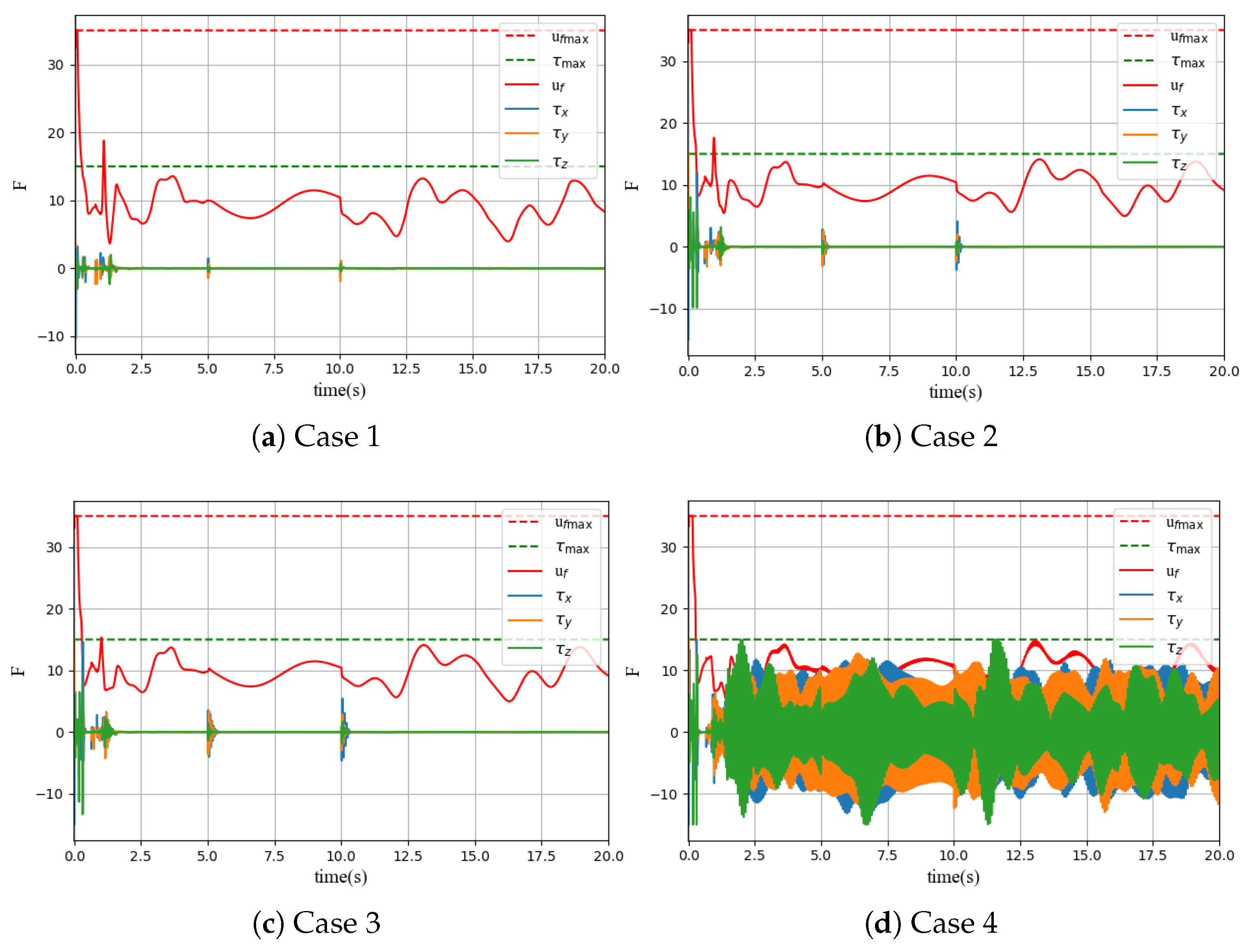
According to the theoretical analysis described above, increasing ${\mathit{\xi }}_{\eta 1}$ and ${\mathit{\xi }}_{\rho 1}$ can improve the robustness of the system. Without the FTDO, four different sets of ${\mathit{\xi }}_{\eta 1}$ are chosen as ${[2.0,2.0,2.0]}^{\top }$ for Case 1, ${[4.0,4.0,4.0]}^{\top }$ for Case 2, ${[5.0,5.0,5.0]}^{\top }$ for Case 3, and ${[8.0,8.0,8.0]}^{\top }$ for Case 4.

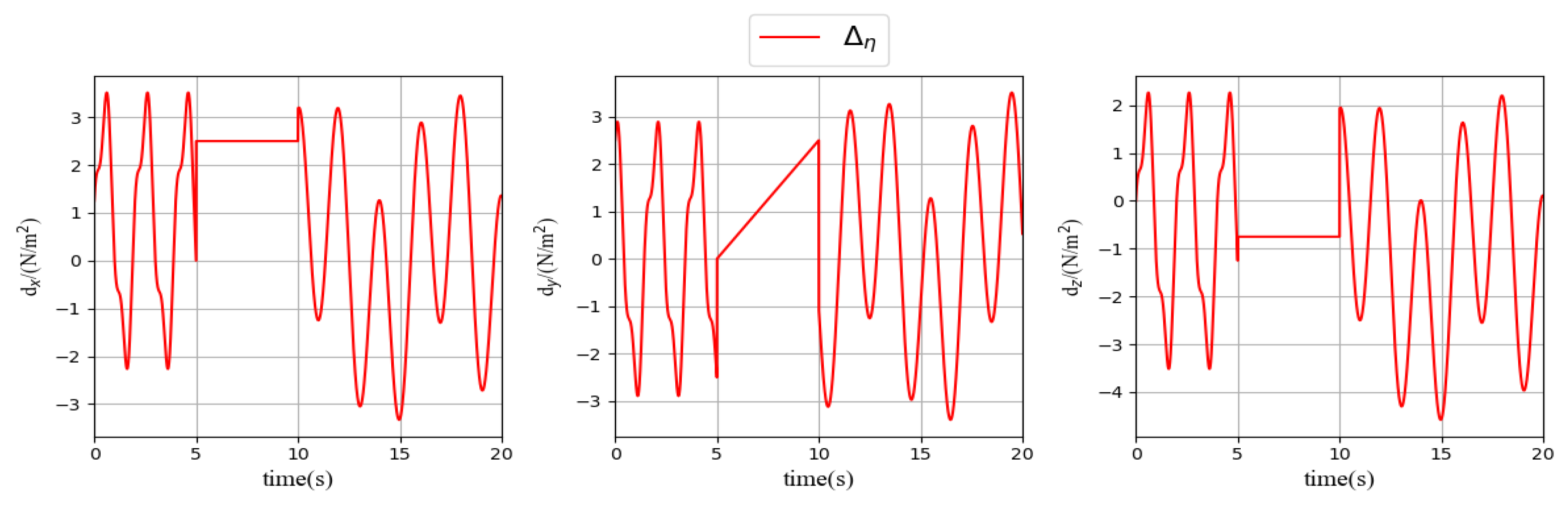
As shown in Figure 3, a variety of disturbances, including sinusoidal disturbances, constant disturbances, and linear time-varying disturbances, are added to the system to verify the robustness of the NFTBS. The bounded $u_f$ and $\mathit{\tau }$ of the QUAVs are depicted in Figure 4, and the dashed red and green lines, respectively, represent the upper bounds of $u_f$ and $\mathit{\tau }$. The response curves of the system are shown in Figure 5.

Figure 3. The disturbances of the translational subsystem.

Figure 4. The constrained inputs.

Figure 5. System response for the controllers with different parameters.

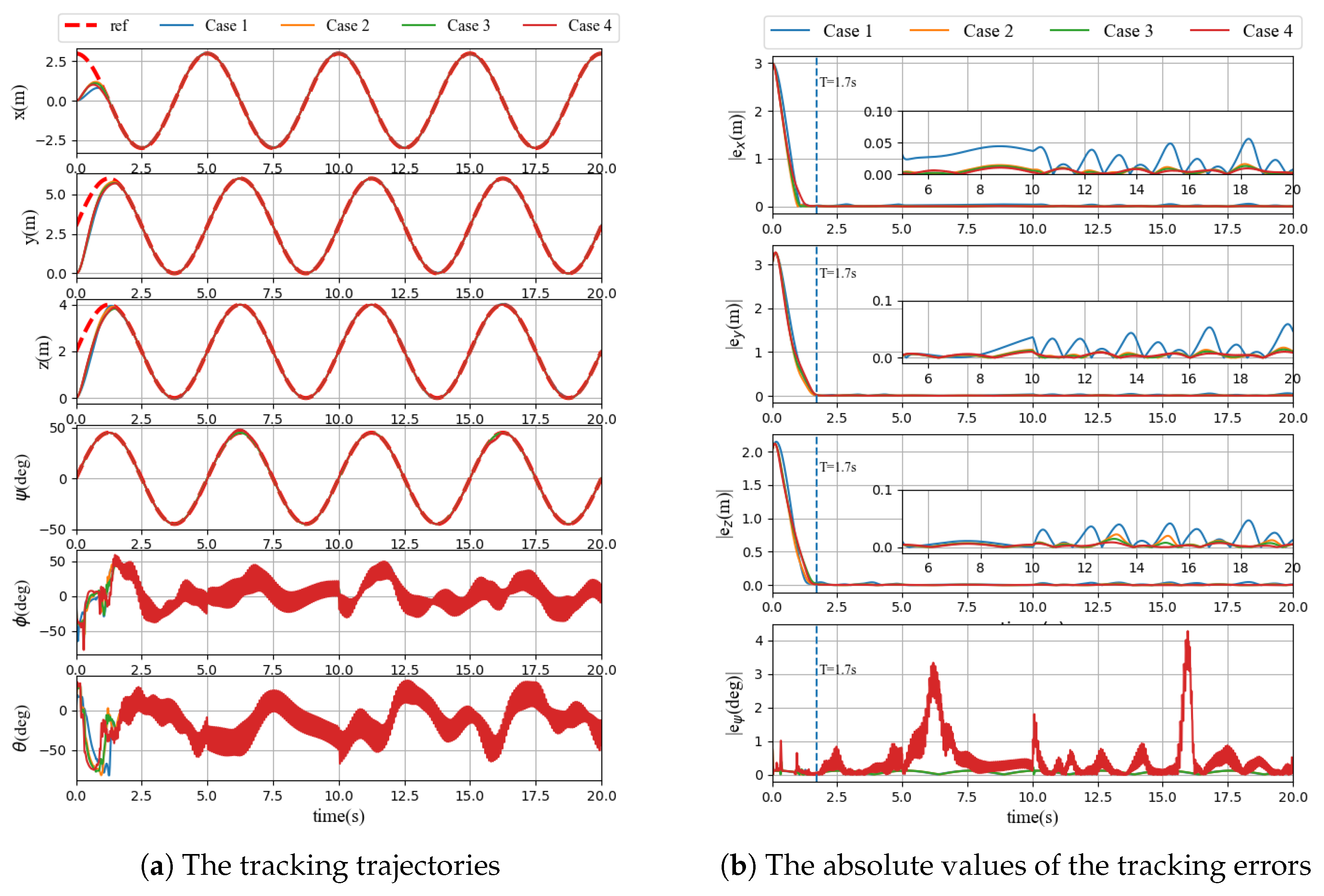
To compare the tracking errors of the system trajectories under different parameters, the average absolute errors $|e_{p1}{|}_{avg}$ and $|e_{\psi 1}{|}_{avg}$ are defined as follows:

$$\begin{array}{cc}\hfill |e_{p1}{|}_{avg}& ={\int }_{t=5}^{10}|e_x{|}^2+ |e_y{|}^2+{|e_z|}^2\mathrm{d}\tau /5,\hfill \\ \hfill |e_{\psi 1}{|}_{avg}& ={\int }_{t=5}^{10}|e_{\psi }{|}^2\mathrm{d}\tau /5,\hfill \end{array}$$

(30)

The tracking errors of the system are measured by calculating the absolute values of the system errors after 5 s. The average errors are listed in Table 1.

Table 1. The mean of the absolute value of the errors.

	Case 1	Case 2	Case 3	Case 4
$|e_{p1}{|}_{avg}\times {10}^{-5}\left({\mathrm{m}}^2\right)$	120.41	8.28	7.40	5.78
$|e_{\psi 1}{|}_{avg}\times {10}^{-3}\left(\mathrm{d}\mathrm{e}{\mathrm{g}}^2\right)$	5.45	5.45	5.45	20.37

Figure 5b and Table 1 demonstrate that increasing ${\mathit{\xi }}_{\eta 1}$ improves the robustness of the system and reduces position tracking error. However, if ${\mathit{\xi }}_{\eta 1}$ becomes too large, it can cause significant oscillations in the input of the rotational loop, as shown in Figure 4d, and substantially increase the tracking error of the yaw angle. Taking all factors into consideration, the parameters of the NFTBS in the following simulations are set in Table 2.

Table 2. Parameters for the NFTBS.

Parameters	Value	Parameters	Value
$p_{\eta }$	0.5	$p_{\rho }$	0.5
${\mathit{k}}_{\eta 11}$	${[1.2,1.2,1.2]}^{\top }$	${\mathit{k}}_{\rho 11}$	${[20.0,20.0,20.0]}^{\top }$
${\mathit{k}}_{\eta 12}$	${[0.2,0.2,0.2]}^{\top }$	${\mathit{k}}_{\rho 12}$	${[1.2,1.2,1.2]}^{\top }$
${\mathit{m}}_{\eta 11}$	${[10.0,10.0,10.0]}^{\top }$	${\mathit{m}}_{\rho 11}$	${[5.0,5.0,5.0]}^{\top }$
${\mathit{k}}_{\eta 21}+{\mathit{\xi }}_{\eta 1}$	${[5.0,5.0,5.0]}^{\top }$	${\mathit{k}}_{\rho 21}+{\mathit{\xi }}_{\rho 1}$	${[40.0,40.0,40.0]}^{\top }$
${\mathit{k}}_{\eta 22}$	${[1.5,1.5,1.5]}^{\top }$	${\mathit{k}}_{\rho 22}$	${[1.5,1.5,1.5]}^{\top }$
${\mathit{m}}_{\eta 21}$	${[5.0,5.0,5.0]}^{\top }$	${\mathit{m}}_{\rho 21}$	${[3.0,3.0,3.0]}^{\top }$

4.2. Fixed-Time Verification for the NFTBS

In this subsection, the fixed-time characteristic of the NFTBS controllers with different initial conditions is shown.

With the same parameters for the nominal system without external disturbances and the actuator failure, set the initial positions as ${\eta }_0={[-2,-2,-2]}^{\top }$ for Case 1, ${\eta }_0={[-1,-1,-1]}^{\top }$ for Case 2, ${\eta }_0={[2,2,2]}^{\top }$ for Case 3, and ${\eta }_0={[3,3,3]}^{\top }$ for Case 4. The response curves of the system are shown in Figure 6.

Figure 6. System response for the different initial conditions.

By Figure 6b, with different initial conditions, all the tracking trajectories of the system can converge in fixed time ($T\le 1.7$ s). The simulation results verify that the controller proposed in this paper can ensure the fixed-time convergence of the system trajectory, without relying on the initial values.

4.3. Comparison of Different Controllers with Actuator Failure

To further highlight the performance of FTDOB-NFTBS for the QUAV system with the extra disturbance and the actuator failure, it is compared with the traditional proportional–integral–derivative (PID), fixed-time proportional–derivative (FTPD) in [37], traditional backstepping (BS) and NFTBS without the disturbance observer. To ensure fairness, the controller parameters are carefully adjusted to achieve uniform convergence times. To thoroughly validate the effectiveness of the algorithm presented in this paper, the simulation is divided into two parts: continuous trajectory tracking and fixed-point tracking.

Case 1: Continuous Trajectories Tracking

A variety of disturbances, as in Figure 3, are added to the system.

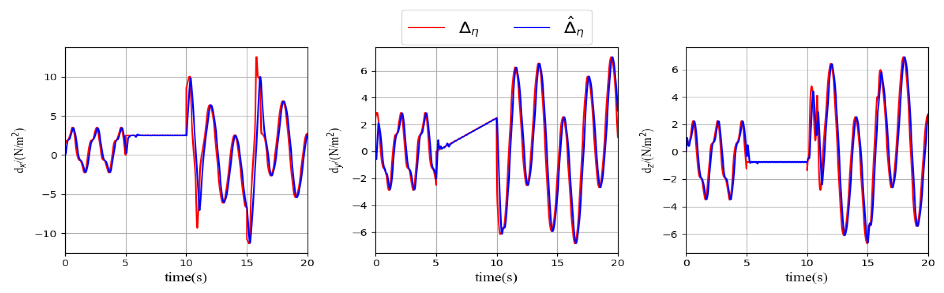
In the simulation, the actuator failure indicators are set to $E_{\eta }=0.5$ and ${\mathit{E}}_{\rho }=\mathrm{diag}(0.5,0.5,0.5)$ after 10 s to demonstrate partial actuator failure. Figure 7 shows the disturbance observer output and the total disturbance, which includes both the extra disturbance and the actuator failure. The red curve represents the true total disturbance, encompassing both the extra disturbance and actuator failure. The blue curve shows the output of the FTDO, while the orange curve represents the true extra disturbance. The noticeable difference between the orange and red curves highlights the impact of the system actuator failure. The results demonstrate that the FTDO used in this paper can quickly and effectively track the total disturbances ${\mathbf{\Delta }}_{\eta }$. Figure 8 displays the system’s constrained inputs, with the dashed red and green lines representing the upper bounds of $u_f$ and $\mathit{\tau }$, respectively. It is important to note that these upper bounds decrease correspondingly as the actuator experiences partial failure.

Figure 7. The disturbances and the observer output.

Figure 8. The constrained inputs.

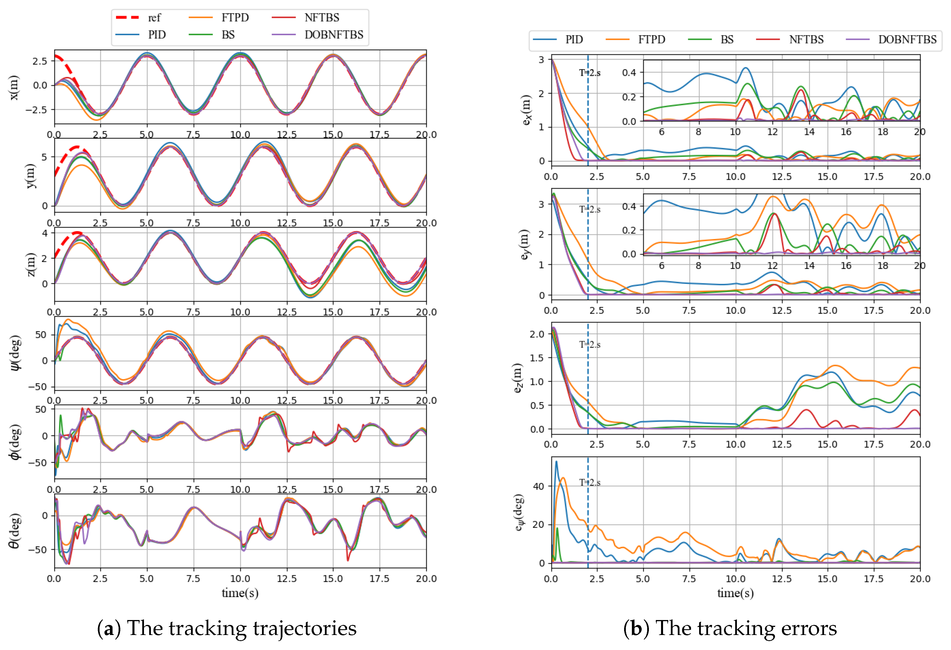
The responses and errors of the system tracking trajectories are depicted in Figure 9. To evaluate the system tracking errors before and after the occurrence of actuator failure, the average absolute errors are defined as

$$\begin{array}{cc}\hfill |e_{p2}{|}_{avg}& ={\int }_{t=5}^{10}|e_x{|}^2+|e_y{|}^2+{|e_z|}^2\mathrm{d}\tau /5,\hfill \\ \hfill |e_{p3}{|}_{avg}& ={\int }_{t=10}^{20}|e_x{|}^2+|e_y{|}^2+{|e_z|}^2\mathrm{d}\tau /10,\hfill \\ \hfill |e_{\psi 2}{|}_{avg}& ={\int }_{t=5}^{10}|e_{\psi }{|}^2\mathrm{d}\tau /5,\hfill \\ \hfill |e_{\psi 3}{|}_{avg}& ={\int }_{t=10}^{20}|e_{\psi }{|}^2\mathrm{d}\tau /10,\hfill \end{array}$$

(31)

where $|e_{p2}{|}_{avg}$ and $|e_{\psi 2}{|}_{avg}$ are defined to evaluate the system tracking errors within 5–10 s without actuator failure. $|e_{p3}{|}_{avg}$ and $|e_{\psi 3}{|}_{avg}$ are defined to evaluate the system tracking errors within 10–20 s when the actuator failure occurs. The results are listed in Table 3.

Figure 9. System response for the different controllers.

Table 3. The mean of the absolute value of the errors.

	PID	FTPD	BC	NFTBS	FTDOB-NFTBS
$|e_{p2}{|}_{avg}\left({\mathrm{m}}^2\right)$	0.26415	0.01019	0.02145	0.00011	0.00006
$|e_{p3}{|}_{avg}\left({\mathrm{m}}^2\right)$	2.05642	2.95152	1.71243	0.05364	0.00049
$|e_{\psi 2}{|}_{avg}\left(\mathrm{d}\mathrm{e}{\mathrm{g}}^2\right)$	22.38140	97.71323	0.02686	0.00534	0.00534
$|e_{\psi 3}{|}_{avg}\left(\mathrm{d}\mathrm{e}{\mathrm{g}}^2\right)$	13.33856	16.18935	0.00130	0.00564	0.00582

In summary, all controllers are capable of stabilizing the QUAV in the absence of actuator failure. However, the errors observed with the NFTBS controller and the FTDOB-NFTBS controller are significantly smaller compared with the other three controllers. Furthermore, Figure 9b shows that the tracking errors with the NFTBS and FTDOB-NFTBS controllers converge to very small regions within 2 s. When actuator failure occurs, the yaw angle tracking errors remain relatively unchanged across all five controllers. However, the position tracking errors with the PID, FTPD, and BC controllers become unacceptably large, with errors along the Z-axis exceeding 1 m. The FTDOB-NFTBS controller exhibits the best performance, with its position tracking error being nearly one-tenth of that of the NFTBS. This highlights the effectiveness of the proposed FTDOB-NFTBS control framework, which demonstrates superior performance in quickly and accurately tracking the reference signal while mitigating the effects of external disturbance and actuator failure.

Case 2: Fixed-Point Tracking

Similar to Case 1, the actuator failure indicators are set to $E_{\eta }=0.5$ and ${\mathit{E}}_{\rho }=\mathrm{diag}(0.5,0.5,0.5)$ after 10 s to demonstrate partial actuator failure. Figure 10 shows the disturbance observer output and the total disturbance, which includes both the extra disturbance and the actuator failure. The red curve represents the true total disturbance, encompassing both the extra disturbance and actuator failure. The blue curve shows the output of the FTDO. Figure 11 displays the system’s constrained inputs, with the dashed red and green lines representing the upper bounds of $u_f$ and $\mathit{\tau }$, respectively. It is important to note that these upper bounds decrease correspondingly as the actuator experiences partial failure.

Figure 10. The disturbances and the observer output.

Figure 11. The constrained inputs.

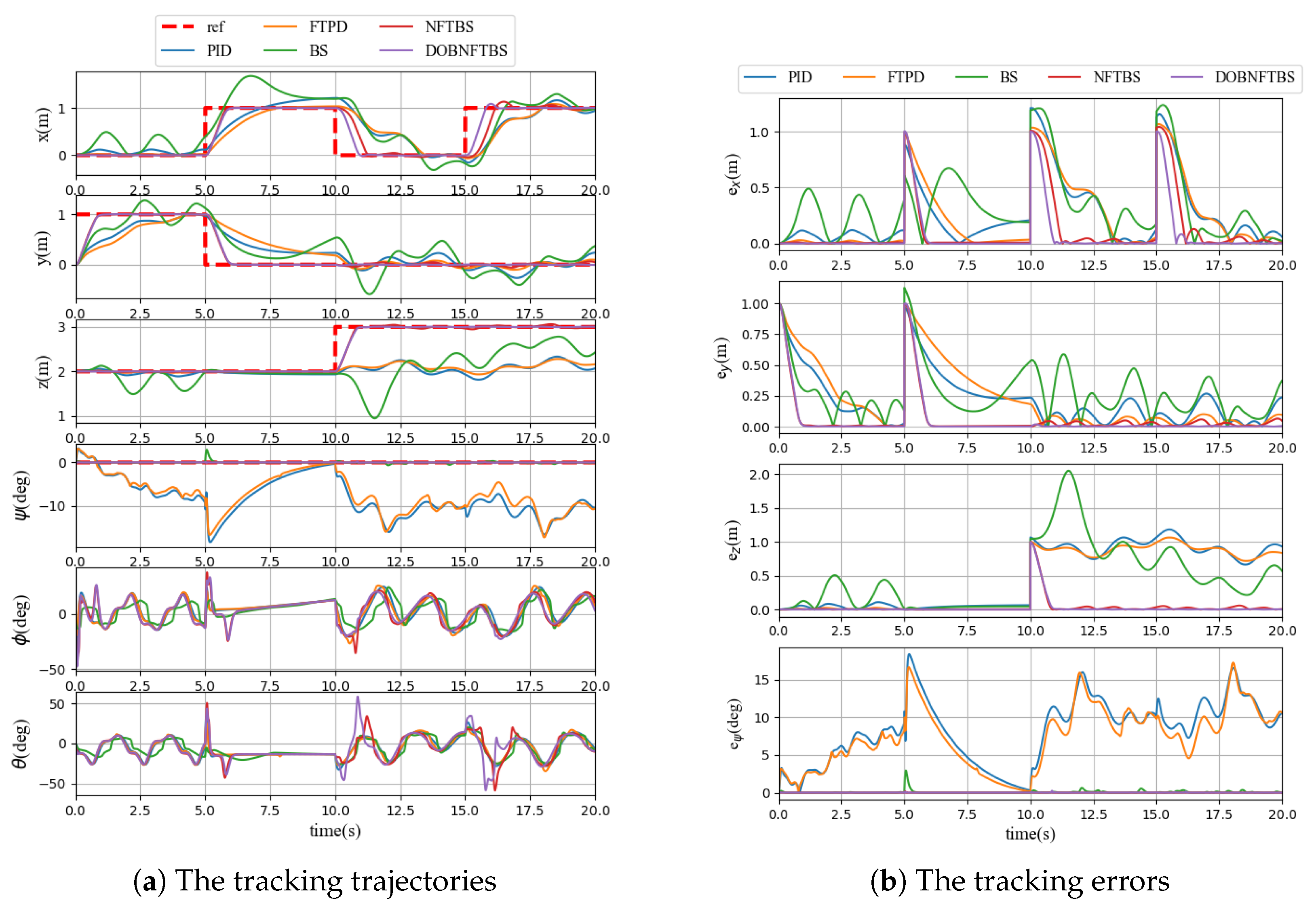
The responses and errors of the system tracking trajectories are depicted in Figure 12. The average absolute errors are defined as (31), and the results are listed in Table 4.

Figure 12. System response for the different controllers.

Table 4. The mean of the absolute value of the errors.

	PID	FTPD	BC	NFTBS	FTDOB-NFTBS
$|e_{p2}{|}_{avg}\left({\mathrm{m}}^2\right)$	0.03800	0.005310	0.13152	8.56048 $\times {10}^{-5}$	7.51011 $\times {10}^{-6}$
$|e_{p3}{|}_{avg}\left({\mathrm{m}}^2\right)$	0.99980	0.92244	0.87783	0.03901	0.01470
$|e_{\psi 2}{|}_{avg}\left(\mathrm{d}\mathrm{e}{\mathrm{g}}^2\right)$	36.57489	29.35372	2.5053 $\times {10}^{-5}$	5.20860 $\times {10}^{-11}$	4.29421 $\times {10}^{-11}$
$|e_{\psi 3}{|}_{avg}\left(\mathrm{d}\mathrm{e}{\mathrm{g}}^2\right)$	711.16298	586.32013	0.00994	4.05917 $\times {10}^{-6}$	3.08465 $\times {10}^{-6}$

In summary, all controllers are capable of stabilizing the QUAV in the absence of actuator failure. However, the errors observed with the NFTBS controller and the FTDOB-NFTBS controller are significantly smaller compared with the other three controllers. The error convergence speed is also significantly faster than other controllers. Furthermore, Figure 12b shows that the tracking errors with the NFTBS and FTDOB-NFTBS controllers can always converge to very small regions within 2 s for suddenly changed reference points. When actuator failure occurs, the position tracking errors with the PID, FTPD, and BC controllers become unacceptably large, with errors along the Z-axis around 1 m. The FTDOB-NFTBS controller exhibits the best performance, with its position tracking error being less than half of that of the NFTBS. This highlights the effectiveness of the proposed FTDOB-NFTBS control framework, which demonstrates superior performance in quickly and accurately tracking the reference signal while mitigating the effects of external disturbance and actuator failure, even for the suddenly changed reference points.

5. Conclusions

This paper presents an FTDOB-NFTBS framework with continuous input for QUAVs that can effectively address challenges such as disturbance, input saturation, and actuator failure. The control framework guarantees the system’s practical stability within a fixed time and successfully avoids singularity and differential explosion issues. By integrating an auxiliary variable, the proposed control framework efficiently compensates for input saturation, while additional controls effectively suppress filter errors. Simulation results highlight the potential and effectiveness of this proposed control framework.

Considering the practical application of the algorithm, in our future work, we plan to incorporate the measurement noise of system states into the closed-loop control system. Furthermore, inspired by [38,39], we will explore extending the proposed algorithm to handle model-uncertain QUAV control. This extension aims to tackle the challenge of achieving high-performance control for unmanned aerial vehicles (UAVs) when system model parameters, such as mass and moment of inertia, are unknown.